Modelling and interpreting the dependence of clustering on the spectral energy distributions of galaxies

Abstract

We extend our previous physically-based halo occupation distribution models to include the dependence of clustering on the spectral energy distributions of galaxies. The high resolution Millennium Simulation is used to specify the positions and the velocities of the model galaxies. The stellar mass of a galaxy is assumed to depend only on $M_{infall}$, the halo mass when the galaxy was last the central dominant object of its halo. Star formation histories are parametrized using two additional quantities that are measured from the simulation for each galaxy: its formation time ($t_{form}$), and the time when it first becomes a satellite ($t_{infall}$). Central galaxies begin forming stars at time $t_{form}$ with an exponential time scale $\tau_{c}$. If the galaxy becomes a satellite, its star formation declines thereafter with a new time scale $\tau_{s}$. We compute 4000 Å break strengths for our model galaxies using stellar population synthesis models. By fitting these models to the observed abundances and projected correlations of galaxies as a function of break strength in the Sloan Digital Sky Survey, we constrain $\tau_{c}$ and $\tau_{s}$ as functions of galaxy stellar mass. We find that central galaxies with large stellar masses have ceased forming stars. At low stellar masses, central galaxies display a wide range of different star formation histories, with a significant fraction experiencing recent starbursts. Satellite galaxies of all masses have declining star formation rates, with similar e–folding times, $\tau_{s}\sim 2.5$ Gyr. One consequence of this long e–folding time is that the colour–density relation is predicted to flatten at redshifts $>1.5$, because star formation in the majority of satellites has not yet declined by a significant factor. This is consistent with recent observational results from the DEEP and VVDS surveys.

1 Introduction

The most fundamental metric of a galaxy is its luminosity, which serves as a rough indicator of its total mass. Another fundamental metric of a galaxy is its colour or spectral type, which is usually interpreted as an indicator of its recent star formation history (although metallicity and dust are both known to affect galaxy colours). In the local Universe, galaxy luminosities and colours are known to be strongly correlated; luminous elliptical galaxies are much redder than the less luminous spirals. It has also long been known that the clustering of galaxies is a strong function of morphological type (Hubble, 1936; Abell, 1958; Davis & Geller, 1976; Dressler, 1980; Loveday et al., 1995; Zehavi et al., 2002), spectral type (Loveday et al., 1999; Norberg et al., 2002; Madgwick et al., 2003), and colour (Willmer et al., 1998; Zehavi et al., 2002; Budavári et al., 2003). On the other hand, galaxy clustering also depends on luminosity (Hamilton, 1988; Park et al., 1994; Willmer et al., 1998; Zehavi et al., 2002), with luminous galaxies being more strongly clustered than fainter ones.

Recent large surveys such as 2dfGRS (Colless et al., 2001) and SDSS (York et al., 2000) have allowed the covariance between galaxy luminosity and colour to be broken. Norberg et al. (2002) showed at all luminosities, galaxies with spectral features indicative of a “passive” old stellar population have higher correlation amplitude than galaxies with ongoing star formation. Likewise Zehavi et al. (2005) and Li et al. (2006a) measured the clustering of red and blue galaxies as a function of luminosity and stellar mass, and showed that red galaxies are more strongly correlated and have a correlation function with a steeper slope. The strongest differences between the red and blue correlation functions occurred for galaxies with the lowest luminosities and stellar masses.

In order to interpret these results, we need to understand the underlying physics that causes the dependence of the correlation function on colour/spectral type. Semi-analytic models of galaxy formation are able to provide considerable insight into the processes that determine how galaxies with different properties cluster (Kauffmann et al., 1997, 1999; Benson et al., 2000; Croton et al., 2006). These models use N-body simulations of the dark matter to specify the locations of galaxies, and they invoke simple prescriptions to describe processes such as gas cooling, star formation and supernova feedback.

In the semi-analytic models (SAMs), there are two reasons why galaxies transition from star-forming (blue) to passive (red) systems. One is a consequence of the infall of a galaxy onto a larger halo. When this occurs, the galaxy is stripped of its supply of infalling gas and its star formation rate declines as its cold gas reservoir is depleted. This means that there will be a population of red satellite galaxies located in groups and clusters (Diaferio et al., 2001). However, this process by itself is not sufficient to explain the very strong observed dependence of colour on galaxy luminosity. Some other process must act to terminate star formation in the central galaxies of massive dark matter haloes. In recent models (Croton et al., 2006; Bower et al., 2006; Cattaneo et al., 2006), feedback from active galactic nuclei (AGN) has been invoked as a possible mechanism for suppressing star formation in massive central galaxies. However, the details of the AGN feedback process and the truncation of star formation in infalling satellite galaxies remain poorly constrained, so in reality there is still considerable freedom when attempting to specify the star formation histories of galaxies in these models. The colour distributions generated by the SAMs should thus be treated as indicative rather than quantitative predictions of the models.

The Halo Occupation Distribution (HOD) approach bypasses any consideration of the physical processes important in galaxy formation. It specifies how galaxies are related to dark matter halos in a purely statistical fashion. van den Bosch et al. (2003) was the first to model the clustering properties of early and late-type galaxies in the context of HOD models by using observational data from the 2dF redshift survey to constrain the average number of early and late-type galaxies of given luminosity residing in a halo of given mass. More recently, Zehavi et al. (2005) built HOD models that were able to reproduce the correlation function of red and blue galaxies as a function of luminosity, by defining a blue galaxy fraction as a function of dark halo mass. The blue fraction also depended on whether the galaxy was a central or a satellite system. The results of both studies demonstrate that the strong clustering of faint red galaxies can be explained if nearly all of them are satellite systems in high-mass halos. These results have recently been extended to higher redshifts by Phleps et al. (2006). The main disadvantage of the HOD approach is that it remains unclear how one progresses from a purely statistical characterization of the link between galaxies and dark matter halos, to a more physical understanding of the galaxy formation process itself.

In previous work (Wang et al., 2006), we attempted to build a physically-based HOD model that would combine the advantages of the statistical HOD models with those of the semi-analytic approach. A large high resolution N-body simulation, the Millennium Simulation (Springel et al., 2005) was used to follow the merging paths of dark matter halos and their associated substructures and to specify the positions and the velocities of the galaxies in the simulation box. The properties of the galaxies (in this case, their luminosities and stellar masses) were specified using simple parameterized functions. Wang et al. (2006) chose to parametrize the luminosities and masses of the galaxies in their models in terms of the quantity $M_{infall}$, which was defined as the mass of the dark matter halo when the galaxy was last the central galaxy of its own halo. Wang et al. (2006) tested this parametrization using the semi-analytic galaxy catalogues of Croton et al. (2006) and and then applied it to data from the Sloan Digital Sky Survey. They were able to show that the relation between stellar mass and halo mass inferred from the combination of the models and the clustering data was in good agreement with independent measurements of this relation using galaxy-galaxy lensing techniques (Mandelbaum et al., 2006).

In this paper, we extend our method to model the dependence of clustering on the spectral energy distributions of galaxies. For galaxies of given stellar mass, we assume the star formation history to depend not only on stellar mass, but also on whether the galaxy is a central object or a satellite in the simulation. We fit this model to the colour distributions of galaxies of give stellar mass, as well as to their correlation functions split by colour. We choose to focus on the spectral index D$4000$ rather than a more traditional broad-band colour. The D$4000$ index is defined as the ratio of the flux in two bands at the long– and short–wavelength side of the $4000$Å  discontinuity. This $4000$Å  break arises from a sum of many absorption lines produced by ionized metals in the atmosphere of stars. Because the absorption increases with decreasing stellar temperature, the D$4000$ break gets larger with older ages, and is largest for old and metal–rich stellar populations. Therefore it is a good indicator of the star formation history of a galaxy. In this work we adopt the narrow definition of the $4000$Å  break introduced by Balogh et al. (1999), and denote it as D${}_{n}4000$. Galaxies with large and small values of D${}_{n}4000$ are referred to as “old” and “young” respectively. Because D${}_{n}4000$ is defined in a narrow wavelength interval, it is insensitive to the effects of dust.

The parametrized models that we construct extend the old ones in which stellar mass $M_{*}$ is assumed to depend only on $M_{infall}$ by assuming that the star formation history of each galaxy declines exponentially after its first appearance in the simulation with time constant $\tau_{c}(M_{*})$ as long as it is a central galaxy, and then with a different time constant $\tau_{s}(M_{*})$ after it becomes a satellite galaxy. Note that this strongly resembles the approach adopted in the semi-analytic models. The main difference is that the time scales $\tau_{c}$ and $\tau_{s}$ and their dependence on mass are not specified using any fixed “recipe”; we allow these time scales to be directly constrained by the observational data. As we will see, this approach allows us to draw interesting physical conclusions from a comparison of our models with the SDSS data.

In Sec. 2 we present observational results from the Sloan Digital Sky Survey (SDSS). These include the D${}_{n}4000$/colour distributions of galaxies in different stellar mass ranges and the projected two point correlation function of red/blue and old/young galaxies. In Sec. 3, we outline our basic theoretical concepts and describe how we decided to model the star formation histories of the galaxies, and calculate their spectral energy distributions. In Sec. 4 we describe how we fit the models to the data. Interpretation and tests of our results are given in Sec. 5. Conclusions and discussions are presented in the final section.

2 The observational results

Our observational results are based on a sample of $\sim$200,000 galaxies drawn from the SDSS Data Release Two. The galaxies have $0.01<z<0.3$, $14.5<r<17.77$ and $-23<M_{{}^{0.1}r}<-16$, where $r$ is the $r$-band Petrosian apparent magnitude corrected for foreground extinction, and $M_{{}^{0.1}r}$ is the $r$-band absolute magnitude corrected to redshift $z=0.1$. This sample has formed the basis of our previous investigations of the correlation function, the power spectrum, pairwise velocity dispersion distributions, and the luminosity and the stellar mass function of galaxies (Li et al., 2006a, b). In Wang et al. (2006), we made use of the measurements of the projected correlation function for galaxies in bins of luminosity and stellar mass to constrain the relation between galaxy luminosity/stellar mass and $M_{infall}$. In this paper, we extend this analysis to the spectral energy distributions of galaxies. In this section, we focus on the distributions of $D_{n}4000$ and colour and we explore how thee projected two-point correlation functions split by $D_{n}4000)$ and colour change as a function of $M_{*}$.

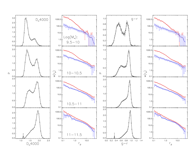
Figure 1: Observational results from SDSS in bins of stellar mass. The left two columns show D${}_{n}4000$ distributions and correlation functions split by D${}_{n}4000$. Red/blue lines represent subsamples with larger/smaller values of D${}_{n}4000$. The right two columns are for $g-r$; the red and blue lines here represent clustering of red and blue subsamples.

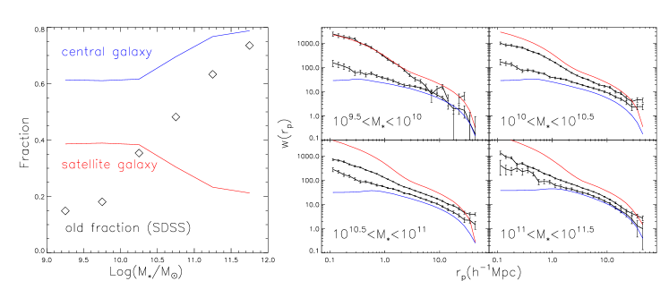
Figure 2: Left panel: fractions of central (blue) and satellite (red) systems in bins of stellar mass in the models of Wang et al. (2006). Black symbols show the fraction of galaxies in the high D${}_{n}4000$ peak from SDSS. Right panel: the clustering of central (blue) and satellite (red) galaxies in the model compared with low/high D${}_{n}4000$ subsamples in the SDSS (upper and lower black curves ).

The galaxies in our sample are divided into four subsamples according to their stellar mass. Each of the stellar mass subsamples is then divided into two further subsamples according to D${}_{n}4000$ and $g-r$, using a method similar to that adopted in Li et al. (2006a). We fit bi-Gaussian functions to the distribution of D${}_{n}4000$ and $g-r$ as a function of stellar mass. The division into high D${}_{n}4000$ and low D${}_{n}4000$, red and blue, is defined to be the mean of the two Gaussian centres in each stellar mass bin. In the computation of the D${}_{n}4000$ and $g-r$ distributions, we have corrected for incompleteness by weighting each galaxy a factor of $V_{survey}/V_{max}$. $V_{survey}$ is the volume for the sample, and $V_{max}$ is the maximum volume over which the galaxy could be observed within the sample redshift range and within the range of $r$-band apparent magnitudes.

For each subsample, the redshift-space two point correlation function(2PCF) $\xi^{s}(r_{p},\pi)$ is measured using the Hamilton (1993) estimator. The projected 2PCF $w(r_{p})$ is then estimated by integrating $\xi^{s}(r_{p},\pi)$ along the line-of-sight direction $\pi$, with $|\pi|$ ranging from 0 to 40 $h^{-1}$ Mpc. When computing 2PCFs, two different methods for constructing random samples have been used: the “standard” method in which the redshift selection function is explicitly modelled using the luminosity function, and the more “general” method in which only the sky positions of the observed galaxies are randomly re-assigned. As shown in Li et al. (2006a), the 2PCFs obtained with the two methods are in good agreement, and here we will use the more “general” method. We have also carefully corrected for possible biases, such as the variance in mass-to-light ratio and the small-scale deficiency in the 2PCF due to fibre collisions (Li et al., 2006a). This ensures accurate measurements for correlation functions on small scales.

To take into account the effect of “cosmic variance” on the $w(r_{p})$ measurements, we have constructed a set of 10 mock galaxy catalogues from the Millennium simulation with exactly the same geometry and selection function as the real sample. The effect of cosmic variance is modelled by placing a virtual observer randomly inside the simulation box when constructing these mock catalogues. The detailed procedure for constructing these mock catalogues has been presented in Li et al. (2006c). For each mock catalogue, we divide galaxies into subsamples according to stellar mass and $g-r$ colour, in the same way as for the real sample, and we measure $w(r_{p})$ for these subsamples. The $1\sigma$ variation between these mock catalogues is then added in quadrature to the bootstrap errors. Note that the errors are assumed to be the same for the splits by $g-r$ and by D${}_{n}4000$.

Fig. 1 shows the distributions of D${}_{n}4000$ and $g-r$ colour for galaxies, as well as the projected 2PCF $w(r_{p})$ for the “red” and “blue” subsamples in four stellar mass ranges. As can be seen, in each stellar mass interval, D${}_{n}4000$/$g-r$ shows a bimodal distribution, with the fraction of galaxies in the red peak increasing towards higher masses. Older/redder galaxies of all stellar masses are more strongly clustered and have steeper correlation functions than their younger/bluer counterparts. This age/colour dependence is much stronger for the low mass galaxies than for the high mass galaxies, particularly on small scales. Notice that the clustering for subsamples split by $D_{n}4000$ and $g-r$ are quite similar, but the distribution functions of these two quantities are quite different, particularly at low masses. For example, for the lowest mass bin ($9.5<\log(M_{*}/M_{\odot})<10$), the fractions of red and blue galaxies are comparable, but the fraction of galaxies with large D${}_{n}4000$ values is much smaller than that of the low D${}_{n}4000$ population. When building our model, we will first focus on the D${}_{n}4000$ spectral index, and test to what extent a model that reproduces the observed trends as a function of D${}_{n}4000$ will also work for $g-r$ colour.

3 theoretical concepts

In the paper of Wang et al. (2006), we used the Millennium Simulation to construct a model to describe the clustering of galaxies as a function of their luminosities and stellar masses. The positions and velocities of the galaxies in the simulation box were obtained by following the orbits and merging histories of the substructures in the simulation. Parametrized functions were then adopted to relate the luminosities and stellar masses of the galaxies to the quantity $M_{infall}$, defined as the mass of the halo at the epoch when the galaxy was last the central dominant object in its own halo. By fitting both the stellar mass function and the projected correlation function $w(r_{p})$ measured in five different stellar mass bins, we were able to use the SDSS data to constrain the link between galaxy stellar mass $M_{*}$ and $M_{infall}$. This relation was parametrized using a double power-law of the form:

$${{M}_{*}}=\frac{2}{(\frac{{M}_{infall}}{{{M}_{0}}})^{-\alpha}+(\frac{{M}_{infall}}{{{M}_{0}}})^{-\beta}}{\times}{k},$$

The scatter in $\log(M_{*})$ at a given value of $M_{infall}$ was described using a Gaussian function with width $\sigma$. Our best-fit model to the SDSS data had the following parameters: $M_{0}=4.0\times 10^{11}h^{-1}M_{\odot}$, $\alpha=0.29$, $\beta=2.42$, $\log{k}=10.35$ and $\sigma=0.203$ for central galaxies and $M_{0}=4.32\times 10^{11}h^{-1}M_{\odot}$, $\alpha=0.232$, $\beta=2.49$, $\log{k}=10.24$ and $\sigma=0.291$ for satellite galaxies.

In this paper, our aim is to extend this model to describe not only the masses and luminosities of galaxies, but also their colours and spectral energy distributions. A successful model should be able to reproduce the 4000 Å break strength distribution at each stellar mass, as well as the correlation functions split by D_n(4000) shown in Fig. 1.

In standard semi-analytic models, galaxies that reside at the centre of their dark matter halo are called central galaxies, and those that have been accreted into larger structures are termed satellite galaxies. The simplest model one could imagine for differentiating galaxies in the high/low D${}_{n}4000$ or red/blue peaks of the bimodal distributions shown in Fig. 1 would be that these two peaks correspond to these satellite and central galaxy populations. Central galaxies have young stellar populations and more active star formation because of ongoing cooling and gas accretion. Satellite galaxies are older because they run out of gas after they are accreted or their gas is removed by processes such as ram pressure stripping. In early semi-analytic models (Kauffmann et al., 1993; Cole et al., 1994; Somerville & Primack, 1999), this was indeed the case; red galaxies were mainly satellite galaxies and blue galaxies were the central galaxies of their own haloes.

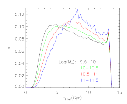
Figure 3: Distribution of infall times for satellite galaxies in different stellar mass bins. The x-axis shows time from past to present, with 13.7Gyr corresponding to the present day.

Fig. 2 shows that this picture does not fit the SDSS observations. In the left panel of Fig. 2, blue and red lines show the fraction of central and satellite galaxies as a function of stellar mass in the model of Wang et al. (2006). For comparison, diamonds show the fraction of galaxies in the high D${}_{n}4000$ peak as a function of $M_{*}$, as measured from the SDSS data. As can be seen, the fraction of satellite galaxies in the simulation does not match the fraction of “old” galaxies in the real Universe, except at stellar masses $\sim 10^{10}M_{\odot}$. At lower stellar masses, the fraction of satellite galaxies is higher than the fraction of old galaxies, implying that some low mass satellite systems are still forming stars. At high stellar masses, nearly all galaxies in the real Universe are “old”. Fig. 2 shows that the majority of these massive old galaxies must be central galaxies.

In the right panel of Fig. 2, blue and red lines show the projected two-point correlation functions for central and satellite galaxies in the simulations in 4 different stellar mass ranges. Results from the SDSS for the low and high D${}_{n}4000$ subsamples are plotted in black. This again shows the failure of a simple central/satellite dichotomy as a way of explaining the difference between the “old” and “young” galaxy populations in the SDSS. As can be seen, the difference in clustering amplitude between the two galaxy populations decreases as a function of increasing stellar mass, while the difference in clustering strength between central galaxies and satellite galaxies remains approximately constant.

It is important to remember that satellite galaxies were not all “created” at the same time. Fig. 3 shows distributions of the times at which satellite galaxies of different stellar masses were first accreted by a larger structure. The satellite infall(i.e. accretion) times $t_{infall}$ are randomly distributed between the two simulation snapshots when the galaxy first transitions from a being central object in its own halo to a satellite system. As can be seen, high mass satellites have on average been accreted more recently than low mass satellites. This effect goes in the wrong direction to resolve the discrepancies shown in Fig. 2. As we have discussed, a substantial number of low mass satellite galaxies are required to have “young” stellar populations, but Fig. 3 shows that low mass satellites typically become satellites quite early on.

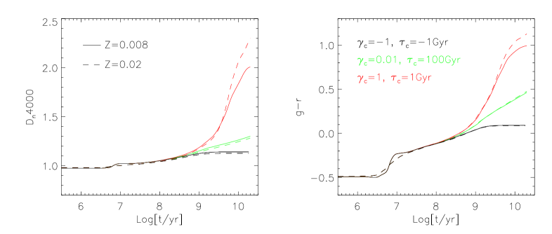
Figure 4: The evolution of D${}_{n}4000$/$g-r$ as a function of time for different values of the star formation timescale parameter $\tau_{c}$ for typical central galaxies. Solid lines are for solar metallicity and dashed lines show results for 0.25 solar metallicity. The coloured lines show results for three different values of $\tau_{c}$.

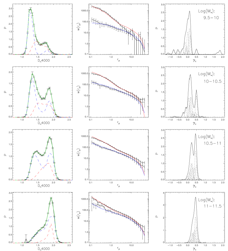
Figure 5: Our best fits to the D${}_{n}4000$ distributions and the correlation functions split by D${}_{n}4000$ in different stellar mass bins. In the left panels, green lines are the full fits, while red/blue dashed lines show the contributions from satellite/central galaxies. In the middle panels, red/blue lines are best-fit correlation functions for subsamples with larger/smaller value of D${}_{n}4000$. The SDSS results are shown in black. The right panels show the the distributions of $\gamma_{c}$ recovered by our non-parametric technique, with dashed lines showing the contribution of each individual Gaussian.

Table 1: Best–fit parameter values for star formation histories in four stellar mass bins as derived from SDSS D${}_{n}4000$ distribution and galaxy correlation functions split by D${}_{n}4000$.

$log(M_{*}/M_{\odot})$	$\gamma_{k}$	$k$	$<\gamma_{c}>_{median}$	$\tau_{c}(Gyr)(50\%,16\%,84\%)$	$<\tau_{s}>(Gyr)$	$\sigma_{\tau_{s}}$	${\Xi}$	$\chi^{2}_{dis}/N_{dis}$
9.5-10	[-1.6,2.2]	77	0.025	(39.97, -4.589, 5.767)	2.312	0.992	4.214	3.126
10-10.5	[-1,1.2]	45	0.175	(5.724, 69.95, 2.106)	2.364	1.041	4.014	2.639
10.5-11	[-1,1]	41	0.318	(3.147, 6.900, 2.081)	2.491	0.534	5.267	4.239
11-11.5	[-0.8,1.2]	41	0.411	(2.435, 3.845, 1.953)	2.103	0.082	7.061	5.837

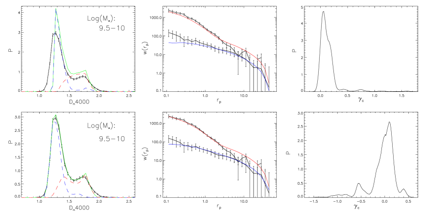
Figure 6: Upper panels: the best fit when $\gamma_{c}$ is constrained to take on positive values. Lower panels: the best fit when $\gamma_{c}$ is constrained to lie below a value of 0.5. Results are shown only for the lowest stellar mass bin: $10^{9.5}-10^{10}M_{\odot}$.

4 PARAMETRIZATION OF THE STAR FORMATION HISTORIES OF GALAXIES IN THE MODEL

4.1 Computation of the SEDs

Recent semi-analytic models (Croton et al., 2006; Bower et al., 2006; Kang et al., 2006; Cattaneo et al., 2006) have attempted to resolve some of the difficulties outlined in the previous section by including “AGN feedback”. The main effect of this form of feedback is to move the central galaxies of massive dark matter haloes to the red sequence. Our approach is different; rather than assume some process that suppresses star formation in massive galaxies, we parametrize the star formation histories of the galaxies in our simulation using simple functions, and we allow the parameters of our model to be constrained by the SDSS data.

The formation time of each galaxy is defined as the time when the halo of the galaxy is first found in the simulation. We also know the infall times of all satellite galaxies, i.e. the times when they first became satellites. To model the star formation histories of our galaxies, we assume that the star formation rate of a galaxy declines exponentially with time after its formation and depends on the stellar mass (at redshift $0$) of the galaxy. We also assume that if a galaxy is accreted and becomes a satellite, its star formation therafter declines with a different e-folding time $\tau_{s}(M_{*})$. The model therefore has two timescales $\tau_{c}(M_{*})$ for central galaxies $\tau_{s}(M_{*})$ for satellite galaxies.

The star formation rate of a galaxy can thus be written:

$${SFR(t)}=\left\{\begin{array}[]{ll}e^{-t/\tau_{c}}&\mbox{, central galaxies}\\ e^{-t_{central}/\tau_{c}}e^{-(t-t_{central})/\tau_{s}}&\mbox{, satellite galaxies}\end{array}\right.$$

where the age of a galaxy $t$ is calculated starting from its formation time $t_{formation}$, which is assigned to a random time between the simulation snapshot when the halo of the galaxy was first found and the immediately preceding snapshot. $t_{central}=t_{infall}-t_{formation}$, is the time that the galaxy spends as the central object of its own halo.

The resulting spectral energy distributions (SEDs) of the galaxies in the simulation are computed using the stellar population synthesis model of BC03 (Bruzual & Charlot, 2003), assuming a Chabrier (2003) IMF. Spectral properties such as the 4000 Å break strength and colour depend on the metallicity of the galaxy as well as on its star formation history. Gallazzi et al. (2005) show that there exists a relation between stellar metallicity and stellar mass for galaxies in the local Universe. We use the mean relation derived in their paper to specify the metallicity of the galaxies in our simulation at a given value of $M_{*}$. Fig. 4 shows the evolution of D${}_{n}4000$/$g-r$ with time for three different values of the $\gamma_{c}$ parameter ($\gamma_{c}$=1/$\tau_{c}(Gyr)$) for a typical central galaxy in our model. Results are shown for solar metallicity BC03 models (solid curves), as well as for 0.25 solar models (dashed curves). As can be seen, there is a small but significant dependence of D${}_{n}4000$ and $g-r$ on metallicity, particularly for galaxies with short star formation time scales. Note also that this computation of the spectral energy distribution neglects the effects of dust on the light emitted by the galaxy. In the following sections, we will concentrate on the 4000 Å break strength, because of its very weak dependence on dust.

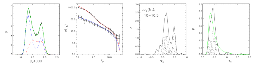
Figure 7: The results of a full non–parametric fit to the distribution of star formation timescales of satellite and central galaxies in the stellar mass range $10^{10}-10.^{10.5}M_{\odot}$. In the right panel, the black curve shows the result of the non-parametric method, while the green line is from the best-fit Gaussian of $\tau_{s}$.

4.2 Fitting the Data

For each galaxy in the Millennium simulation, we have determined $t_{formation}$ and $t_{infall}$. We have also built a “library” of predicted present-day D${}_{n}4000$ values by running the BC03 models for different combinations of galaxy metallicity $z$, galaxy lifetime, and the two star formation time scales $\tau_{c}$ and $\tau_{s}$. We interpolate over the grid of parameter values stored in the library to obtain D${}_{n}4000$ for all the galaxies in the simulation. In addition, we know the (x,y,z) positions of the galaxies within the simulation volume , and their stellar masses have already been specified using the model developed as part of our previous study (Wang et al., 2006). We therefore have all the necessary ingredients to calculate the D${}_{n}4000$ distributions as well as the correlation functions split by D${}_{n}4000$ for different ranges in stellar mass and to compare the model predictions with the observations.

Initially we attempted to parametrize the distributions of $\tau_{c}$ and $\tau_{s}$ using simple Gaussian functions. However, this resulted in rather poor fits to the data. Further experimentation indicated that it would be advantageous to switch to a method that would allow the distributions of $\tau_{c}$ and $\tau_{s}$ to take on complex shapes. Following the methodology outlined by Blanton et al. (2003), the distribution of $\gamma_{c}=1/\tau_{c}$ is parameterized by a sum of many Gaussians with mean values $\gamma_{k}$ equally distributed in a given range:

$${P(\gamma_{c})}=\sum{N_{k}\frac{1}{\sqrt{2\pi\sigma^{2}}}e^{{-\frac{1}{2}(\frac{\gamma_{c}-\gamma_{k}}{\sigma})^{2}}}}{/}\sum{N_{k}}$$

We assume the same scatter $\sigma$ for each Gaussian, but allow the weighting factors $N_{k}$ to vary. For each stellar mass interval, the range and number of Gaussians used in this non-parametric fitting technique are listed in Table 1. The central values $\gamma_{k}$ of each Gaussian are equally distributed over the range with a step of $0.05$. $\sigma$ for each Gaussian is fixed to be the same as this step width. This method allows the distribution of $\gamma$ values to take on any shape. This approach turned out to be critical for central galaxies, but resulted in little improvement when applied to the satellite population (see Sec. 5.1). We therefore employ the non-parametric method only for the central galaxies. For satellite galaxies, a simple Gaussian centred at $<\tau_{s}>$ and with the scatter of $\sigma_{\tau_{s}}$ is used to parametrize the distribution of $\tau_{s}$.

During the fitting procedure, we also noticed that constraining $\gamma_{c}$ to be positive did not allow us to reproduce the blue end of D${}_{n}4000$ distribution. We therefore allowed the parameter $\gamma_{c}$ to take on both positive and negative values. In practice, a negative value of $\gamma_{c}$ corresponds to a galaxy that is experiencing an elevated level of star formation at the present day (i.e. a starburst). For satellite galaxies, the time scale $\tau_{c}$ is constrained to be positive, which is in any case preferred by our fits.

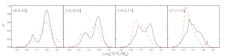
Figure 8: The distribution of specific star formation rates predicted by our model (red dashed lines) is compared with results derived from the SDSS (black solid lines), in different stellar mass bins.

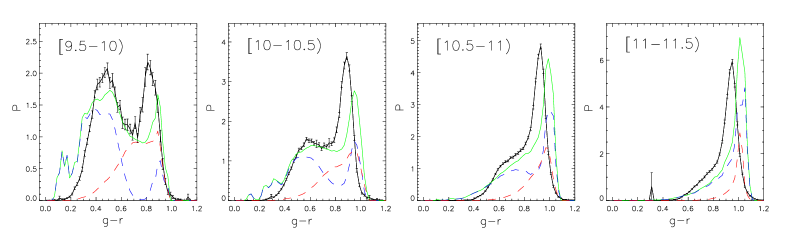
Figure 9: $g-r$ distributions predicted by our model compared to results from the SDSS. The green curves show the full distribution, while the red and blue dashed curves show the contributions from satellite and central galaxies. Black curves show results from the SDSS.

To find a best-fit to both the D${}_{n}4000$ distribution and the galaxy correlation functions split by D${}_{n}4000$, we employ the Levenberg-Marquardt algorithm, which interpolates between the Gauss-Newton algorithm and the method of gradient descent. The final results of the fitting procedure are shown in Fig. 5. For each stellar mass bin, D${}_{n}4000$ distributions and correlation functions for high/low D${}_{n}4000$ subsamples are shown together with the distribution of $\gamma_{c}$ that produces the best fit. In the left panel, blue and red dashed curves show results for central and satellite galaxies, while green lines are for both types of galaxy. In the middle panel, red and blue curves refer to high and low D${}_{n}4000$ subsamples defined using the same technique that was applied to the SDSS data. The distribution of $\gamma_{c}$ that results in these fits is shown in the right panels. Table 1 lists the parameters of the best fit models for four stellar mass bins. For central galaxies, the median value of $\gamma_{c}$ is listed, as well as the timescale $\tau_{c}=1/\gamma_{c}$, its median value and its 16 and 84 percentile values. The table also lists $<\tau_{s}>$ and $\sigma_{\tau_{s}}$, the parameters that describe the star formation histories of satellite galaxies. We estimate our parameters by minimizing the quantity:

$${\Xi}=\frac{{\chi}^{2}_{dis}}{N_{dis}}+\frac{{\chi}^{2}_{corr}}{N_{corr}}$$

with

$${{\chi}^{2}_{dis}}=\sum_{N_{dis}}{\left[\frac{P-P_{SDSS}}{\sigma(P_{SDSS})}\right]^{2}}$$

and

$${{\chi}^{2}_{corr}}=\sum_{N_{corr}}{\left[\frac{w(r_{p})-w(r_{p})_{SDSS}}{\sigma(w(r_{p})_{SDSS})}\right]^{2}}$$

where ${\chi}^{2}_{dis}$ is evaluated for the D${}_{n}4000$ distribution and ${\chi}^{2}_{corr}$ is evaluated for the projected correlation functions of the high and the low D${}_{n}4000$ subsamples. For each stellar mass bin, $N_{dis}$ is the number of points along the D${}_{n}4000$ distribution that we fit. In practice, we adopt $N_{dis}=50$ with D${}_{n}4000$ in the range [0.5,3]. $N_{corr}$ is the number of points on the correlation function used in the fit. We adopt $N_{corr}=20\times 2$ with $r_{p}$ ranging from $0.113$ to $8.972h^{-1}$ Mpc.

5 THE RESULTS

5.1 Discussion of the Results

From Fig. 5 and Table.1, it is clear that star formation histories of low mass and high central galaxies are very different. At large stellar masses ($M_{*}>10^{10.5}M_{\odot}$), nearly all central galaxies have positive $\gamma_{c}$, and a large fraction of them have ceased forming stars. There is a peak in the distribution of $\gamma_{c}$ at a value of around $0.45$, which corresponds to an e–folding timescale of $\sim 2$ Gyr. Together with a minority of old and massive satellite galaxies, these central galaxies in which star formation has shut down are necessary to explain the strong peak in the D${}_{n}4000$ distribution at values of $\sim 1.8$, characteristic of metal-rich, evolved stellar populations.

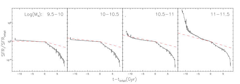
Figure 10: The median star formation histories of satellite galaxies in different stellar mass bins. Black lines show results from the semi-analytic models of De Lucia & Blaizot (2006), while red dashed lines are from our models. The SFR is normalized to its value at the infall time. On the x-axis, the time is plotted relative to $t_{infall}$.

At low stellar masses, galaxies display a much wider variety in star formation history. This is especially true in our lowest stellar mass bin ($9.5<\log(M_{*}/M_{\odot})<10$). Nearly half the galaxies in this mass range have negative $\gamma_{c}$. In addition, there are also some objects that have “switched off’, i.e. the distribution of $\gamma_{c}$ exhibits a tail toward large positive values.

In the upper panel of Fig. 6 we show what happens to our fit in this stellar mass range if $\gamma_{c}$ is forced to take on only positive values. The fitting procedure is exactly the same as described in Sec.4, but $\gamma_{k}$ is constrained to lie in the range $[0.05,2]$. The result shows that the blue end of the D${}_{n}4000$ distribution is not well fit without a population of “star-bursting” galaxies. In the BC03 model, a constant star formation rate will result in a D${}_{n}4000$ value of no less than $\sim 1.2$ for a galaxy with an age of a few Gyrs (see green lines in Fig. 4). It is thus not possible to obtain low enough values of D${}_{n}4000$ to match the observations, unless we allow for negative values of $\gamma_{c}$.

In the lower panel of Fig. 6, we test what happens if we do not allow the distribution of $\gamma_{k}$ to extend to very large positive values. If we truncate the distribution at a value of 0.5, we still find fairly good fit with ${\Xi}=4.836$, which is comparable to our best-fit model. This implies that the existence of a long tail of galaxies with large positive values of $\gamma_{k}$ is not strongly preferred, i.e. our model is not sensitive to the exact timescale over which the star formation was truncated in these “old” central galaxies. One possibility is that these galaxies correspond to a post-starburst phase in which star formation has been temporarily reduced following exhaustion of the gas or blow-out of a significant fraction of the interstellar medium.

From the values of $\tau_{s}$ listed in Table 1, it can be seen that unlike central galaxies, satellite galaxies of all masses have similar e–folding timescales, with an average value of around $2-2.5$ Gyr. This indicates that all satellite galaxies experience a similar decline in star formation rate after falling into a large structure. To test the robustness of this conclusion, and to see if a Gaussian is sufficient to describe the dispersion in $\tau_{s}$ values, we have carried out a full non-parametric fit to constrain the shape of both the $\gamma_{c}$ and the $\gamma_{s}$($\gamma_{s}=1/\tau_{s}$) distributions for galaxies in the stellar mass range $10^{10-10.5}M_{\odot}$. The results are shown in Fig. 7, with the panel on the far right showing the derived distribution of $\gamma_{s}$. The distribution of $\gamma_{s}$ obtained using the non-parametric fitting method is somewhat different to the simple Gaussian fit (indicated on the plot by the green curve). Nevertheless, the resulting median value of $\tau_{s}$ is $2.257$ Gyr, which is about the same as that of the simple Gaussian fit. The small difference in the distribution of $\tau_{s}$ between the two methods makes very little difference to the fit or to the resulting $\Xi$ values.

5.2 Consistency Checks

So far, we have tuned the parameters $\tau_{c}$ and $\tau_{s}$ to reproduce the D${}_{n}4000$ distributions of SDSS galaxies as a function of stellar mass and the projected correlation functions of high D${}_{n}4000$ and low D${}_{n}4000$ galaxy subsamples. We have chosen to focus on D${}_{n}4000$ because it is relatively insensitive to the effects of dust. However, D${}_{n}4000$ is only one of many possible age-indicators, so it is interesting to check whether we obtain consistent results for other measures of the star formation history of a galaxy.

Brinchmann et al. (2004) computed specific star formation rates (i.e. the star formation rate per unit stellar mass) for SDSS galaxies. For star-forming galaxies, the values were derived using emission line fluxes suitably corrected for the effects of dust, so this indicator of recent star formation history is independent of D_n4000. For galaxies with absent or very weak emission lines, the specific star formation rates were in fact estimated using the D${}_{n}4000$ index, so this is no longer an independent measure. Nevertheless it is interesting to test whether the distribution of SFR/$M_{*}$ predicted by our best-fit model is in agreement with the results derived directly from the SDSS data.

In Fig. 8, we show the results of this test. The red dashed curves in the figure show the distributions of the specific star formation rates predicted by our best fit model in four different bins of stellar mass. To calculate these values, we simply integrate the star formation rate over the lifetime of a galaxy to get its total stellar mass and we then divide the star formation rate at the present day by this value. The fraction of stellar mass that is returned to the interstellar medium over the lifetime of the galaxy is taken to be $0.5$, which is the median value predicted by the BC03 model. The black lines show the results obtained directly from our SDSS sample, which have beed corrected for volume incompleteness with the $1/V_{max}$ weighting scheme (the same method as for computing D${}_{n}4000$ and $g-r$ distributions described in Sec. 2). From the plot we see that the agreement between our model “predictions” and the observations is reasonably good. The qualitative trends as a function of stellar mass are reproduced quite well, but the absolute values of the specific star formation rate predicted by the model tend to be somewhat lower than in the data.

We now test whether the same models allow us to reproduce the colour distributions of galaxies. As we have noted, galaxy colours are quite sensitive to the effects of dust, so it would be surprising to us if this were the case!

Fig. 9 shows the predicted $g-r$ colour distributions in the absence of dust and indeed, it appears that the model does not fit very well. At low stellar masses, the model produces too many extremely blue galaxies and not enough galaxies in the red peak. This tells us that a substantial number of galaxies in this red peak are actually star-forming galaxies that are strongly reddened by dust. At high stellar masses, the predicted shape of the $g-r$ colour distribution is similar to the observations, but there is an offset in the predicted colours of galaxies in the red peak as compared to the observations. The existence of an offset in $g-r$ of around $0.1$ mag for high stellar mass galaxies has been noted several times in the literature on stellar population models (see section 2.4.3 in Gallazzi et al. (2005) and appendix of BC03 for more details about this colour mismatch for galaxies with old stellar populations). One possibility is that the offset is related to the effects of non-solar element abundance ratios on the SEDs, something which is not currently accounted for by the BC03 models.

In summary, our results show that although very similar qualitative results are obtained when using different spectral indicators, there are non-negligible quantitative differences. In particular, the effects of dust on galaxy colours must be taken into account when interpreting colour distributions and the clustering properties of galaxies split by colour. This problem is not as serious for high mass galaxies, which are mainly ellipticals with little gas, ongoing star formation or dust. However, it is a major issue for low mass galaxies, where the shapes of the distribution of D${}_{n}4000$ and $g-r$ are quite different. As we have already seen from Fig. 1, the relative fractions of high/low D_n4000 and red/blue galaxies also differ substantially in our lowest mass bins.

5.3 Comparison with the Results of Semi-analytic Models

As discussed in Sec. 1, the star formation histories of galaxies predicted by modern semi-analytic models ought to be similar to those in our model. In the SAMs, the star formation rates of galaxies also decline after they transition from central galaxies to satellite systems. In addition, modern SAMs also incorporate AGN feedback mechanisms that act to shut down star formation in the central galaxies of massive dark matter halos. It is interesting to investigate whether there is “quantitative” agreement between our results and those of the semi-analytic models.

In Fig. 10, we compare the median star formation history of satellite galaxies in our model (red dashed lines) with the median star formation history of satellites in the semi-analytic galaxy catalogues of De Lucia & Blaizot (2006)(black lines). Results are shown for four different stellar mass bins. On the x-axis, we plot the time relative to $t_{infall}$. On the y-axis, we plot the star formation rate normalized to its value at $t=t_{infall}$. As can be seen, the main difference between the two models lies in the behaviour of the star formation after the galaxy is accreted as a satellite. In the semi-analytic model, star formation declines much more rapidly than in our model. In our model, the median star formation e-folding time scale of satellites is around $2-2.5$ Gyr, independent of galaxy stellar mass. In the semi-analytic models, the e-folding time is closer to 1 Gyr. The median star formation rates during the phase when the galaxies are central objects are actually quite similar in the two models, except for the very most massive galaxies. In the semi-analytic models, most of the massive galaxies appear to have experienced a short period of very intense star formation in their past, probably reflecting an early phase of gas-rich merging.

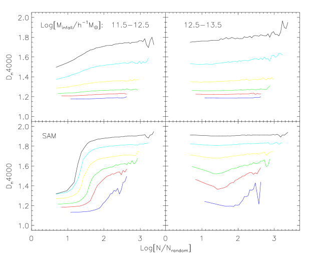
Figure 11: Colour–density relations for our models (upper panels) and for the semi-analytic model(lower panels) in bins of hosting halo mass at the infall time of the galaxy. Coloured lines represent different redshifts: $z=0$, $0.3$, $0.8$, $1.5$, $2$, $3$ from top to bottom in each figure. $N$ and $N_{random}$ refer to number of galaxies within a sphere of radius $2Mpc$ centred on the galaxy and on random positions.

5.4 Evolution to Higher Redshifts

As we showed in the previous section, there are significant differences in the star formation histories of satellite galaxies in our model as compared to the semi-analytic model of De Lucia & Blaizot (2006). As a result, the colours and spectral properties of satellites galaxies in the two models will differ substantially at high redshifts, because the time between $t_{infall}$ and $t_{observation}$ will be considerably smaller than at the present day. If the star formation e-folding timescale of satellite galaxies is long, one would expect many of these systems to be still blue and actively star forming at higher redshifts. Recent work by Cucciati et al. (2006) and Cooper et al. (2006) has found that the steep colour–density relation observed at low redshift becomes weaker and gradually disappears by a redshift of $\sim 1.5$.

In Fig. 11, we plot the relations between D${}_{n}4000$ and local density in our model (upper panels) and in the semi-analytic model (lower panels). Results are shown at 5 different redshifts and for two different ranges in the quantity $M_{infall}$. In the semi-analytic model, D${}_{n}4000$ is calculated using the BC03 model. The local density is evaluated by counting the number of galaxies within a sphere of radius 2 Mpc centred on each galaxy and dividing by the corresponding number in randomly distributed spheres of the same size. We only include galaxies with $M_{infall}$ greater than $2\times 10^{11}h^{-1}M\odot$ when calculating these densities in order to make sure that our results are not affected by the resolution limit of the simulation. Lines with different colours show the median $D_{n}4000$ for galaxies as a function of density at redshifts $z=0$, $0.3$, $0.8$, $1.5$, $2$, $3$. In both models, the D${}_{n}4000$–density relations are shallower for galaxies with higher values of $M_{infall}$, reflecting the fact that the star formation histories for satellite galaxies are rather similar at high masses. However, the evolution with redshift differs substantially in the two models. In our models, the D${}_{n}4000$–density relations become much flatter at higher redshifts and they basically disappear by a redshift of $\sim 1$. In contrast, the relations in the semi-analytic models remain steep up to redshifts $\sim 3$. It is interesting that for galaxies with $M_{infall}>10^{12.5}M_{\odot}$, the trend in colour as a function of density exhibits a non-monotonic behaviour at higher redshifts in the SAM.

The main reason why the colour density relation of low mass galaxies remains steep out to high redshifts in the semi-analytic models is because $\tau_{s}$ is short. As we noted in the previous subsection, at redshift zeros $\tau_{s}$ is $\sim 1$ Gyr in the SAMS as compared to $\sim 2.5$ Gyr for our best-fit model. In SAMs, the star formation rate is assumed to be invesely proportional to the dynamical time of the galaxy and hence, for a given value of $M_{infall}$, $\tau_{s}$ will be smaller at higher redshifts. In our model, we have assumed that $\tau_{s}$ is independent of redshift.

6 Summary and Conclusions

We have extended the physically-based halo occupation distribution (HOD) models of Wang et al. (2006), which relate the stellar mass of the galaxy to the mass of its halo at the time it was last a central dominant object. The models presented in this paper consider the dependence of clustering on the spectral energy distributions (SEDs) of galaxies. The star formation history of a galaxy is assumed to depend on stellar mass and on the time at which the galaxy transitions from being a central galaxy to a satellite galaxy orbiting within a larger structure. The stellar population synthesis model of Bruzual & Charlot (2003) is used to compute the spectral energy distributions of the galaxies in the model. Rather than colour, we focus on the spectral index D${}_{n}4000$ because of its weak dependence on dust. By fitting both the bimodal distribution of D${}_{n}4000$ and the projected correlation functions for high/low D${}_{n}4000$ subsamples for SDSS galaxies in 4 different stellar mass ranges, we constrain the star formation e–folding time of central and satellite galaxies as a function of stellar mass at $z=0$.

Our results show that at high stellar masses, a large fraction of central galaxies have ceased forming stars. This shutdown in star formation is necessary to explain the fact that the majority of massive galaxies are red and old. It is also consistent with the conclusions of Croton et al. (2006); Bower et al. (2006); Cattaneo et al. (2006), who show that a shut-down of gas cooling and star formation in massive dark matter halos results in a much better fit to present-day galaxy luminosity functions and colour distributions. In these models, radio AGN feedback is invoked as the mechanism responsible for this suppression of cooling.

For low stellar masses, central galaxies display a wide range of different star formation histories. A significant fraction of low mass central galaxies are experiencing starbursts. We also find a “tail” of low mass central galaxies in which star formation is currently suppressed, but our model is not sensitive to exactly when this suppression occurred. In a recent paper, Kauffmann et al. (2006) studied the star formation histories of local galaxies by analysing the scatter in their colours and spectral properties, and concluded that star formation occurs in shorter, higher amplitude events in smaller galaxies. It is interesting that we come to very similar conclusions using a completely different method. Compared to central galaxies, satellites have a much narrower distribution of star formation e–folding timescales. In satellites, the average e-folding time does not depend on stellar mass and has a value of around $2-2.5$ Gyr.

We have also checked whether our best–fit model parameters derived from the distributions and clustering of galaxies as a function of D${}_{n}4000$ can be extended to understanding the distribution of galaxy colours. Our conclusion is that the effects of dust must be taken into account when modelling colours. This is especially true of low mass galaxies, which can be actively star-forming and yet contain sufficient dust to match the colours of high mass ellipticals.

Finally, we have compared the star formation histories of galaxies in our model with the semi-analytic models of galaxy formation od De Lucia & Blaizot (2007). The main difference between the two approaches is in the timescale over which star formation declines in satellite galaxies once they are accreted by larger structures. In the semi-analytic models, star formation in satellites decreases with an e-folding time of about $1$ Gyr. In our models, the decrease occurs on a timescale that is a factor of $2-3$ times longer. This leads to a conflict between the colours of satellites in the models and in the SDSS data. Similar conclusions have been reached by Weinmann et al. (2006), who show that the semi-analytic models of Croton et al. (2006) predict a blue fraction of satellites that is too low to match results from their catalogue of galaxy groups extracted from the SDSS.

Assuming our derived star formation parameters to apply at all times , we predict a weakening of the colour–density relation towards higher redshifts and a complete disappearance of this relation at redshift of about $1.5$. This is consistent with recent work by Cucciati et al. (2006) and Cooper et al. (2006). In contrast, a strong colour–density relation is maintained in the De Lucia & Blaizot (2007) semi-analytic model up to redshifts greater than $3$.

References

- Abell (1958) Abell G. O., 1958, ApJS, 3, 211
- Balogh et al. (1999) Balogh M. L., Morris S. L., Yee H. K. C., Carlberg R. G., Ellingson E., 1999, ApJ, 527, 54
- Benson et al. (2000) Benson A. J., Baugh C. M., Cole S., Frenk C. S., Lacey C. G., 2000, MNRAS, 316, 107
- Blanton et al. (2003) Blanton M. R., Hogg D. W., Bahcall N. A., Brinkmann J., Britton M., Connolly A. J., Csabai I., Fukugita M., et al., 2003, ApJ, 592, 819
- Bower et al. (2006) Bower R. G., Benson A. J., Malbon R., Helly J. C., Frenk C. S., Baugh C. M., Cole S., Lacey C. G., 2006, MNRAS, 370, 645
- Brinchmann et al. (2004) Brinchmann J., Charlot S., White S. D. M., Tremonti C., Kauffmann G., Heckman T., Brinkmann J., 2004, MNRAS, 351, 1151
- Bruzual & Charlot (2003) Bruzual G., Charlot S., 2003, MNRAS, 344, 1000
- Budavári et al. (2003) Budavári T., Connolly A. J., Szalay A. S., Szapudi I., Csabai I., Scranton R., Bahcall N. A., Brinkmann J., et al., 2003, ApJ, 595, 59
- Cattaneo et al. (2006) Cattaneo A., Blaizot J., Weinberg D. H., Colombi S., Dave R., Devriendt J., Guiderdoni B., Katz N., Keres D., 2006, astro-ph/0605750
- Chabrier (2003) Chabrier G., 2003, PASP, 115, 763
- Cole et al. (1994) Cole S., Aragon-Salamanca A., Frenk C. S., Navarro J. F., Zepf S. E., 1994, MNRAS, 271, 781
- Colless et al. (2001) Colless M., Dalton G., Maddox S., Sutherland W., Norberg P., Cole S., Bland-Hawthorn J., Bridges T., et al., 2001, MNRAS, 328, 1039
- Cooper et al. (2006) Cooper M. C., Newman J. A., Coil A. L., Croton D. J., Gerke B. F., Yan R., Davis M., Faber S. M., et al., 2006, astro-ph/0607512
- Croton et al. (2006) Croton D. J., Springel V., White S. D. M., De Lucia G., Frenk C. S., Gao L., Jenkins A., Kauffmann G., Navarro J. F., Yoshida N., 2006, MNRAS, 365, 11
- Cucciati et al. (2006) Cucciati O., Iovino A., Marinoni C., Ilbert O., Bardelli S., Franzetti P., Le Fèvre O., Pollo A., et al., 2006, A&A, 458, 39
- Davis & Geller (1976) Davis M., Geller M. J., 1976, ApJ, 208, 13
- De Lucia & Blaizot (2006) De Lucia G., Blaizot J., 2006, astro-ph/0606519
- Diaferio et al. (2001) Diaferio A., Kauffmann G., Balogh M. L., White S. D. M., Schade D., Ellingson E., 2001, MNRAS, 323, 999
- Dressler (1980) Dressler A., 1980, ApJ, 236, 351
- Gallazzi et al. (2005) Gallazzi A., Charlot S., Brinchmann J., White S. D. M., Tremonti C. A., 2005, MNRAS, 362, 41
- Hamilton (1988) Hamilton A. J. S., 1988, ApJ, 331, L59
- Hamilton (1993) Hamilton A. J. S., 1993, ApJ, 417, 19
- Hubble (1936) Hubble E. P., 1936, Yale University Press
- Kang et al. (2006) Kang X., Jing Y. P., Silk J., 2006, ApJ, 648, 820
- Kauffmann et al. (1999) Kauffmann G., Colberg J. M., Diaferio A., White S. D. M., 1999, MNRAS, 303, 188
- Kauffmann et al. (2006) Kauffmann G., Heckman T. M., De Lucia G., Brinchmann J., Charlot S., Tremonti C., White S. D. M., Brinkmann J., 2006, MNRAS, 367, 1394
- Kauffmann et al. (1997) Kauffmann G., Nusser A., Steinmetz M., 1997, MNRAS, 286, 795
- Kauffmann et al. (1993) Kauffmann G., White S. D. M., Guiderdoni B., 1993, MNRAS, 264, 201
- Li et al. (2006b) Li C., Jing Y. P., Kauffmann G., Börner G., White S. D. M., Cheng F. Z., 2006b, MNRAS, 368, 37
- Li et al. (2006a) Li C., Kauffmann G., Jing Y. P., White S. D. M., Börner G., Cheng F. Z., 2006a, MNRAS, 368, 21
- Li et al. (2006c) Li C., Kauffmann G., Wang L., White S. D. M., Heckman T. M., Jing Y. P., 2006c, MNRAS, 373, 457
- Loveday et al. (1995) Loveday J., Maddox S. J., Efstathiou G., Peterson B. A., 1995, ApJ, 442, 457
- Loveday et al. (1999) Loveday J., Tresse L., Maddox S., 1999, MNRAS, 310, 281
- Madgwick et al. (2003) Madgwick D. S., Hawkins E., Lahav O., Maddox S., Norberg P., Peacock J. A., Baldry I. K., Baugh C. M., et al., 2003, MNRAS, 344, 847
- Mandelbaum et al. (2006) Mandelbaum R., Seljak U., Kauffmann G., Hirata C. M., Brinkmann J., 2006, MNRAS, 368, 715
- Norberg et al. (2002) Norberg P., Baugh C. M., Hawkins E., Maddox S., Madgwick D., Lahav O., Cole S., Frenk C. S., et al., 2002, MNRAS, 332, 827
- Park et al. (1994) Park C., Vogeley M. S., Geller M. J., Huchra J. P., 1994, ApJ, 431, 569
- Phleps et al. (2006) Phleps S., Peacock J. A., Meisenheimer K., Wolf C., 2006, A&A, 457, 145
- Somerville & Primack (1999) Somerville R. S., Primack J. R., 1999, MNRAS, 310, 1087
- Springel et al. (2005) Springel V., White S. D. M., Jenkins A., Frenk C. S., Yoshida N., Gao L., Navarro J., Thacker R., et al., 2005, Nature, 435, 629
- van den Bosch et al. (2003) van den Bosch F. C., Yang X., Mo H. J., 2003, MNRAS, 340, 771
- Wang et al. (2006) Wang L., Li C., Kauffmann G., de Lucia G., 2006, MNRAS, 371, 537
- Weinmann et al. (2006) Weinmann S. M., van den Bosch F. C., Yang X., Mo H. J., Croton D. J., Moore B., 2006, MNRAS, 372, 1161
- Willmer et al. (1998) Willmer C. N. A., da Costa L. N., Pellegrini P. S., 1998, AJ, 115, 869
- York et al. (2000) York D. G., Adelman J., Anderson J. E., Anderson S. F., Annis J., Bahcall N. A., Bakken J. A., Barkhouser R. a., 2000, AJ, 120, 1579
- Zehavi et al. (2002) Zehavi I., Blanton M. R., Frieman J. A., Weinberg D. H., Mo H. J., Strauss M. A., Anderson S. F., Annis J., et al., 2002, ApJ, 571, 172
- Zehavi et al. (2005) Zehavi I., Zheng Z., Weinberg D. H., Frieman J. A., Berlind A. A., Blanton M. R., Scoccimarro R., Sheth R. K., et al., 2005, ApJ, 630, 1