The Sunyaev-Zel’dovich effects from a cosmological hydrodynamical simulation: large-scale properties and correlation with the soft X-ray signal

Abstract

Using the results of a cosmological hydrodynamical simulation of the concordance $\Lambda$CDM model, we study the global properties of the Sunyaev-Zel’dovich (SZ) effects, both considering the thermal (tSZ) and the kinetic (kSZ) component. The simulation follows gravitation and gas dynamics and includes also several physical processes that affect the baryonic component, like a simple reionization scenario, radiative cooling, star formation and supernova feedback. Starting from the outputs of the simulation we create mock maps of the SZ signals due to the large structures of the Universe integrated in the range $0\leq z\leq 6$. We predict that the Compton $y$-parameter has an average value of $(1.19\pm 0.32)\times 10^{-6}$ and is lognormally distributed in the sky; half of the whole signal comes from $z<1$ and about 10 per cent from $z>2$. The Doppler $b$-parameter shows approximately a normal distribution with vanishing mean value and a standard deviation of $1.6\times 10^{-6}$, with a significant contribution from high-redshift ($z>3$) gas. We find that the tSZ effect is expected to dominate the primary CMB anisotropies for $\ell\ga 3000$ in the Rayleigh-Jeans limit, while interestingly the kSZ effect dominates at all frequencies at very high multipoles ($\ell\ga 7\times 10^{4}$). We also analyse the cross-correlation between the two SZ effects and the soft (0.5–2 keV) X-ray emission from the intergalactic medium and we obtain a strong correlation between the three signals, especially between X-ray emission and tSZ effect ($r_{\ell}\simeq$ 0.8-0.9) at all angular scales.

1 Introduction

In the recent years the cosmic microwave background (CMB) primordial fluctuations have been measured with high accuracy thanks to the observations made by the Wilkinson Microwave Anisotropy Probe satellite (WMAP, Spergel et al., 2003, 2006), establishing an important step forward in precision cosmology. The primary CMB anisotropies, in fact, constitute the most important dataset to obtain information about the physical conditions of the early Universe and, together with other results coming from high-redshift supernovae (see, e.g., Astier et al., 2006; Wood-Vasey et al., 2007), weak lensing (see, e.g., Heymans et al., 2005; Massey et al., 2005; Hetterscheidt et al., 2006; Semboloni et al., 2006; Hoekstra et al., 2006) and galaxy clustering (see, e.g., Cole et al., 2005; Eisenstein et al., 2005; Tegmark et al., 2006; Sánchez et al., 2006), they indicated as a favorite scenario a flat cosmological model dominated by a cosmological constant: the so-called $\Lambda$CDM model.

The dynamical and thermodynamical effects of the large scale structure (LSS) formation after the recombination also create secondary anisotropies in the CMB signal. Most importantly, after the epoch of reionization the CMB photons interact with the free electrons of the intergalactic medium (IGM) via Thomson scattering giving rise to the Sunyaev-Zel’dovich (SZ) effect (Sunyaev & Zel’dovich, 1972, 1980): this constitutes both a noise for the primary CMB signal and a probe for the baryon physics. The SZ effect is usually classified into two components: the dominant one, the thermal SZ (tSZ) effect, is the inverse-Compton scattering caused by the thermal motion of a population of high-temperature electrons, mainly located in the hot plasma of galaxy clusters, which results in a gain in energy for the photons and a consequent distortion of the black-body spectrum of the CMB. Conversely, the kinetic SZ (kSZ) effect is the Doppler shift caused by the bulk motion of the ionized gas and can result either in a gain or in a loss of photon energy, depending on the direction of the gas velocity with respect to the photon.

After its first claimed detection by Parijskij (1973) and the works of Birkinshaw et al. (1991) and Birkinshaw & Hughes (1994), the development of new microwave instruments has now made available a large amount of observational data for the study of the tSZ effect in galaxy clusters, including two-dimensional mapping. In the near future this observational field is believed to receive a significant boost thanks to a new generation of suitable land-based instruments, like AMI, SPT, ACT, SZA, AMiBA and APEX, and the launch of the Planck satellite that will provide a full-sky catalogue of galaxy clusters detected via the tSZ effect. Finally, the project of the Atacama Large Millimeter Array (ALMA) specifically includes high-resolution imaging of the SZ effect in its scientific goals.

The development of the SZ science for galaxy clusters will be strictly connected with the already available data in the X-ray band that nowadays constitute the most important dataset for cluster physics. In fact, since both the bremsstrahlung emission and the SZ effect depend on the density and temperature of the gas, the two signals are expected to be highly correlated and their comparison will be of great interest in order to understand the systematics of the two observables. In addition to it, while the X-ray signal has proven to be a sensitive probe for the properties of the hot gas in the central regions of nearby clusters, the absence of redshift dimming for the SZ effect and its different dependence on the density will allow one to detect more distant sources and, hopefully, to obtain more information on the external regions of galaxy clusters where the modelization of the cluster physics has smaller uncertainties (see, e.g., Roncarelli et al., 2006b). Besides from cluster physics the tSZ effect arising from the whole LSS, which is expected to be the most important signal at the angular scales of some arcminutes, can also be used to directly constrain cosmology because of the strong dependence of its amplitude on the normalization of the power spectrum $\sigma_{8}$ (see, e.g., Goldstein et al., 2003; Bond et al., 2005; Douspis et al., 2006). On the other side a measurement of the kSZ effect can yield information on the peculiar velocity field at high redshift and, consequently, put constraints on different dark energy models (see, e.g., Hernández-Monteagudo et al., 2006) and on cosmological parameters in general (see, e.g., Bhattacharya & Kosowsky, 2007); at the second order the kSZ effect is also believed to be marginally affected by the dynamical effects associated with epoch of reionization, even if a future measurement of this signal appears very challenging (Iliev et al., 2007).

In this framework a theoretical analysis of the SZ effect and of its correlation with the X-ray signal is crucial not only for investigating the connections between these observables and the LSS formation, but also for modeling and, possibly, taking under control the SZ-noise, that is expected to affect high-multipole CMB observations. In this paper we present our results on the statistical properties of the SZ signal obtained from a cosmological hydrodynamical simulation (Borgani et al., 2004) that follows the evolution of the structure formation in the framework of the $\Lambda$CDM cosmology. Since the thermodynamical evolution of the baryons depends not only on the cosmological parameters but also on different non-thermal processes influencing the gas physics, our numerical model specifically includes several physical effects connected with radiative cooling and star formation that have a significant effect on the shape of the temperature and density profiles of the inner regions of galaxy clusters and, consequently, on their X-ray and SZ properties.

This paper is organized as follows. In the next Section we briefly review the basic equations that describe the tSZ and kSZ effects. In Section 3 we present the characteristics of our cosmological simulation (Section 3.1) and the method used to obtain predictions on the SZ effects from its outputs (Section 3.2). In Section 4 we discuss the average large-scale properties of the SZ effects. In Section 5 we analyze the power spectra of the tSZ and kSZ signals and in Section 6 we study their cross-correlation. Section 7 is devoted to the description of the correlation properties with the soft X-ray signal. Finally we summarize our conclusions in Section 8.

2 Basics of the SZ effects

Here we review some of the basic equations for both SZ effects in the non-relativistic approximation. More details can be found in several reviews (see, e.g., Rephaeli, 1995; Birkinshaw, 1999; Carlstrom et al., 2002; Rephaeli et al., 2005).

The intensity of the tSZ effect in a given direction is usually expressed in terms of the Compton $y$-parameter defined as

$$y\equiv\frac{k_{B}\,\sigma_{T}}{m_{e}\,c^{2}}\int{dl\,n_{e}(T_{e}-T_{\rm CMB})}\ ,$$ (1)

where $m_{e}$ is the electron rest mass, $c$ is the light speed, $n_{e}$ and $T_{e}$ are the electron number density and temperature, and $T_{\rm CMB}$=2.726 K is the CMB temperature (Mather et al., 1994). The resulting change in the latter due to the scattering of the electrons is directly proportional to the value of the $y$-parameter and is given by

$$\frac{\Delta T}{T_{\rm CMB}}=y\,g_{\nu}(x)\ ,$$ (2)

where $x\equiv h\,\nu/(k_{B}T_{\rm CMB})$ is the dimensionless frequency and $g_{\nu}(x)$ represents the dependence on the observation frequency:

$$g_{\nu}(x)=\left(x\,\frac{e^{x}+1}{e^{x}-1}-4\right)\ .$$ (3)

It is important to note that in the Rayleigh-Jeans (RJ) limit ($x\ll 1$) this expression reduces to $g_{\nu}(x)\simeq-2$ and that for $\nu\simeq 218$ GHz the tSZ effect is null.

The kSZ effect can be expressed in terms of the Doppler $b$-parameter defined as

$$b\equiv\frac{\sigma_{T}}{c}\int{dl\,n_{e}\,v_{r}}\ ,$$ (4)

where $v_{r}$ is the radial component of the peculiar velocity of the gas element (positive if it is moving away from the observer, negative if it is approaching). The resulting measured temperature fluctuation is $\Delta T/T_{\rm CMB}=-b$. Note that, unlike for the tSZ effect, this is independent of the observation frequency.

3 Models and method

It is known that the global properties of the tSZ and kSZ effects depend on the physical characteristics of the LSS as a whole. Moreover, as we will discuss in Section 4, significant contributions to both SZ effects comes from high-redshift gas. Therefore a theoretical study of their global properties and the comparison with present and future observations require a realistic modelization of the thermodynamical and dynamical history of the gas filling the volume of the past light-cone seen by an observer located at $z=0$ out to the epoch of reionization. For this purpose we use the outputs of a cosmological hydrodynamical simulation at different redshifts to build different realizations of light-cones, which enable the production of simulated maps of the SZ signals.

3.1 The cosmological hydrodynamical simulation

We use the results of the cosmological hydrodynamical simulation by Borgani et al. (2004), which considers the concordance cosmological model, i.e. a flat $\Lambda$CDM model dominated by the presence of the cosmological constant ($\Omega_{\rm m}=0.3$, $\Omega_{\Lambda}=0.7$), with a Hubble parameter $h\equiv H_{0}/$(100 km s^-1 Mpc^-1)=0.7, and a baryon density $\Omega_{\rm b}=0.04$. The initial conditions were generated by sampling from a cold dark matter (CDM) power spectrum, normalized by assuming $\sigma_{8}=0.8$, being $\sigma_{8}$ the r.m.s. matter fluctuation into a sphere of radius $8h^{-1}$ Mpc. The run, that was carried out with the tree-sph code gadget-2 (Springel et al., 2001; Springel, 2005), followed the evolution of $480^{3}$ dark matter (DM) particles and as many gas particles from $z=49$ to $z=0$. The side of the cubic box is $192h^{-1}$ Mpc and correspondingly the masses of the DM and gas particles are $m_{\rm DM}=4.62\times 10^{9}h^{-1}M_{\odot}$ and $m_{\rm gas}=6.93\times 10^{8}h^{-1}M_{\odot}$, respectively. The Plummer-equivalent gravitational softening of the simulation was set to $\epsilon$=7.5 $h^{-1}$ kpc in physical units between $z=2$ and $z=0$, and fixed in comoving units at higher redshifts. This run produced one hundred outputs, equally spaced in the logarithm of the expansion factor, between $z=9$ and $z=0$.

The simulation treats not only gravity and non-radiative hydrodynamics, but also includes different processes that can influence the physics of the intracluster medium (ICM), like star formation (by adopting a sub-resolution multiphase model for the interstellar medium; see Springel & Hernquist, 2003), feedback from type II supernovae (SN-II) with the effect of galactic outflows, radiative cooling processes within an optically thin gas of hydrogen and helium in collisional ionization equilibrium and heating (by a uniform, time-dependent, photoionizing UV background expected from a population of quasars and modelled following Haardt & Madau, 1996).

The results of this simulation have been used for different previous investigations (see, e.g., Murante et al., 2004; Ettori et al., 2004; Cheng et al., 2005; Rasia et al., 2005). Diaferio et al. (2005) used the whole sample of galaxy clusters extracted from this simulation at $z=0$ to find a good agreement with the observed scaling relations between X-ray and SZ properties and to evaluate the lower limit (about 200 km s^-1) to the systematic errors that will affect future measurements of cluster peculiar velocities with the SZ effect. Recently Roncarelli et al. (2006a) used this simulation and the same light-cone realizations to estimate the soft (0.5–2 keV) X-ray emission arising from the diffuse gas and found a good agreement with the current upper limits of the unresolved X-ray background.

3.2 The map-making procedure

In order to create mock maps of the tSZ and kSZ signals produced by the LSS integrated over redshift, we use the same light-cone simulations analyzed by Roncarelli et al. (2006a) for the study of the X-ray emission. Note that similar applications of the same technique, also in terms of SZ effects, have been done by different authors (see, e.g., da Silva et al., 2000; Croft et al., 2001; da Silva et al., 2001a; da Silva et al., 2001b; Springel et al., 2001; White et al., 2002; Zhang et al., 2002). The method is based on the replication of the original box volume along the line of sight. For the projection we prefer to make use of the comoving coordinates, taking advantage of the fact that in a flat cosmology, like the one here assumed, light travels along a straight line. We build past light-cones extending out to $z=6$. As we will discuss in more detail in Section 4, this limit is enough to account for almost all of the tSZ signal; on the contrary the kSZ effect is believed to have a non-negligible contribution from the gas located at $z>6$, out to the epoch of reionization. Anyway, since the reionization model assumed in our simulation considers the gas at $z\ga 6$ almost neutral, extending the calculation to higher redshifts would not produce a significant change in the kSZ signal. Therefore we stress that the results for the kSZ effect presented in this work cannot be considered as the whole signal expected, but rather as the signal arising from the gas in the range $0\leq z\leq 6$ which, according to the results of Iliev et al. (2007), should constitute the dominating component. The extension of our light-cone realizations corresponds to a comoving distance of approximately $5770\ h^{-1}$ Mpc, so we would need to stack the simulation volume roughly 30 times. However, in order to obtain a better redshift sampling, rather than stacking individual boxes, we adopt the following procedure. Each simulation volume necessary to construct the light-cone is divided along the line of sight into three equal slices, each of them having a depth of $64\ h^{-1}$ Mpc. Then the stacking procedure is done by choosing the slice extracted from the simulation output that best matches the redshift of the central point of the slice. Our light-cones are thus built with 91 slices extracted from 82 different snapshots.

In order to avoid that the same structures are repeated along the line of sight, we include a process of box randomization in our map-making procedure, taking advantage of the periodic boundary conditions of our simulation: for each box entering the light-cone we combine a process of random recentring of the coordinates with a 50 per cent probability of reflecting each axis. In order to avoid spatial discontinuities between slices belonging to the same box, we impose the same randomization process to them: in this way we can retain the global information on the large-scale structures present in the box and at the same time we strongly reduce the loss of large-scale power. In order to extend the field of view of our maps, we replicate the boxes four times across the line of sight starting at comoving distances larger than half the light-cone extension (i.e. larger than about $2900\ h^{-1}$ Mpc, corresponding to $z\ga 1.4$). In this way we are able to obtain maps 3.78^∘ on a side, containing $8192^{2}$ pixels, with a resolution of 1.66 arcsec. Notice that the method to pile up boxes (sketched in Fig. 1) can introduce systematic errors on the calculation of the power spectrum (see the corresponding discussion in Section 5). We apply this method by varying the initial random seeds to produce 10 different light-cone realizations, used to assess the statistical robustness of our results and the influence of cosmic variance.

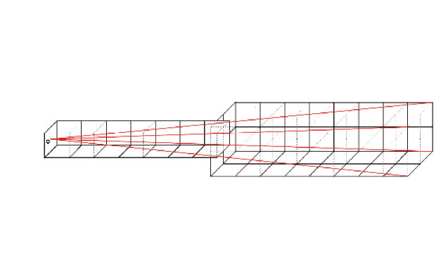
Figure 1: Sketch of the configuration adopted to realize the light-cones. The observer is located at the position $O$ at the centre of the left side of the first box. The past light-cone is obtained by stacking the comoving volumes of the simulation outputs taken at the corresponding redshift. In order to obtain a large field of view of size $3.78^{2}$ deg², starting at $z\simeq 1.4$ we use four replications of the box at the same redshift. The red lines show the volume inside the light cone corresponding to the field of view.

To compute the signal produced by the SZ effects we need to convert the line-of-sight integrals of equations (1) and (4) into expressions suitable for the sph formalism. First, for the tSZ effect, we calculate the contribution of every gas element that lies inside the light-cone volume. We follow an approach similar to the one proposed by da Silva et al. (2000). Given the $i$-th sph particle, we define

$$\Upsilon_{i}\equiv\frac{k_{B}\,\sigma_{T}}{m_{e}\,c^{2}}\,N_{e,i}T_{i}\ ,$$ (5)

where $T_{i}$ is the gas temperature and $N_{e,i}$ is the number of electrons associated to the particle, i.e. $N_{e,i}=n_{e,i}\,m_{i}/\rho_{i}$, being $n_{e,i}$, $m_{i}$ and $\rho_{i}$ the electron density, the mass and the gas density of the $i$-th particle, respectively. Then, according to the required map resolution, we compute the physical length of the pixel $L_{{\rm pix},i}$ at the particle’s distance from the observer and we use it to calculate

$$y_{i}\equiv\frac{\Upsilon_{i}}{L_{{\rm pix},i}^{2}}\ ,$$ (6)

which is the total contribution to the $y$-parameter from the $i$-th particle. This quantity is then distributed over the map pixels by adopting the same sph smoothing kernel which is used in the simulation code for the computation of hydrodynamical forces and proposed by Monaghan & Lattanzio (1985):

$$W(x)\propto\left\{\begin{array}[]{ll}1-6x^{2}+6x^{3},&0\leq x<0.5\ ,\\ 2(1-x)^{3},&0.5<x\leq 1\ ,\\ 0,&x>1.\end{array}\right.$$

In the previous expressions $x\equiv\Delta\theta/\alpha_{i}$, where $\Delta\theta$ represents the angular distance between the pixel centre and the projected particle position and $\alpha_{i}$ is the angle subtended by the particle smoothing length provided by the hydrodynamical code. In order to conserve the total intensity associated to each particle we normalize to unity the sum of the weights $W$ over all involved pixels. Finally, the intensity in a given pixel is obtained by summing over all the particles inside the light-cone.

The construction of the maps of the Doppler $b$-parameter follows an identical procedure with the only difference that we have to substitute equation (5) and (6) with

$$B_{i}\equiv\frac{v_{r,i}}{c}\,N_{e,i}\ ,$$ (7)

and

$$b_{i}\equiv\frac{B_{i}}{L_{{\rm pix},i}^{2}}\ ,$$ (8)

where $v_{r,i}$ is the radial component of the peculiar velocity of the $i$-th particle, which can be either negative or positive.

4 The distribution of the SZ signals

In Fig. 2 we present two examples of the maps of the Compton $y$-parameter (left panel) and Doppler $b$-parameter (right panel) obtained with the method described in the previous section; both refer to the same light-cone simulation.

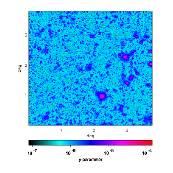
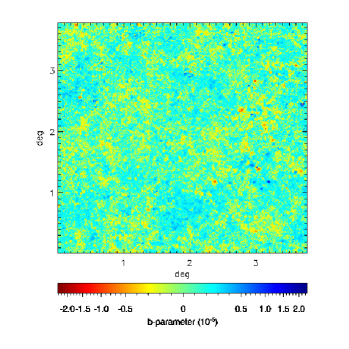
Figure 2: Maps of the tSZ (left panel) and kSZ (right panel) signals expressed in terms of the Compton $y$-parameter and Doppler $b$-parameter (given in units of $10^{-5}$), respectively. The maps are 3.78^∘ on a side and the pixel size is (1.66 arcsec)². Both maps refer to the same realization of the past light-cone.

It is evident in the tSZ map that the signal is dominated by galaxy clusters that can reach in their central regions typical intensities close to $y\sim 10^{-4}$, which correspond to temperature changes an order of magnitude higher than the primary CMB anisotropies, in the RJ limit. In the map it is also possible to recognize a large number of smaller and fainter structures with $y\sim 5\times 10^{-6}$: they correspond to distant protoclusters or more local galaxy groups. We also note a non-negligible signal arising from regions outside clusters (e.g. filaments and diffuse gas) that can reach at most $y\sim 10^{-6}$. We use the whole set of maps to compute the expected average of the Compton $y$-parameter: we obtain a value of $<y>=(1.19\pm 0.32)\times 10^{-6}$ as the mean of the pixel values in the 10 fields of $3.78^{2}$ deg²; the reported error represents the r.m.s. in fields of 1 deg². This value is significantly lower than the results obtained by da Silva et al. (2001b, cooling model) and White et al. (2002, cooling plus feedback model): $2.3\times 10^{-6}$ and $2.1\times 10^{-6}$, respectively. The main reason of this discrepancy is the smaller value of $\sigma_{8}$ adopted in our simulation ($\sigma_{8}=0.8$ against their $\sigma_{8}=0.9$): the mean value of the Compton $y$-parameter is in fact expected to scale roughly as $\sigma_{8}^{\alpha/2}$, with $\alpha\approx 4-7$ (see, e.g., Sadeh & Rephaeli, 2004; Diego & Majumdar, 2004). For the same set of maps, we also repeat the analysis but considering only the gas particles of the warm-hot intergalactic medium (WHIM, see Cen & Ostriker, 1999; Davé et al., 2001), defined as the gas component having a temperature $T$ in the range $10^{5}$ $<T<10^{7}$ K and we obtain $<y>_{\rm WHIM}=(6.90\pm 0.42)\times 10^{-7}$, which means that about 60 per cent of the total value of the $y$-parameter is originated by WHIM gas, while the remaining fraction comes from hotter gas ($T>10^{7}$ K).

Analyzing the kSZ map, we notice that the peaks can reach values of $|b|\ga 10^{-5}$, i.e. roughly of the same intensity of the typical $\Delta T/T$ of the primary CMB signal. These peaks correspond to clusters which are not necessarily massive and/or hot like for the tSZ signal, but that have significant bulk motions. This leads to considerable displacements in the peak positions in the two maps: for example, we note that the brightest source in the tSZ map, roughly located in the position (2.2^∘,1.0^∘) and corresponding to a cluster at $z\sim 0.3$, is completely absent in the kSZ maps, since it is a relaxed object with a small radial component of the peculiar velocity.

In Fig. 3 we show the probability distribution function of both SZ signals calculated considering the values in the (1.66 arcsec)² pixels: in particular the thin lines refer to each of the 10 light-cone realizations, while the thick line is the corresponding average. We notice that the tSZ effect distribution is close to a lognormal function while the kSZ one is similar to a gaussian one. Regarding the average distribution of the tSZ signal we computed the first moments of $I_{y}\equiv\log y$: we find $\overline{I_{y}}=-6.07$ with a corresponding r.m.s. of 0.31 and a skewness of 0.96. The odd moments of the kSZ effect average distributions are close to zero, as expected, and we obtain an r.m.s. of $1.3\times 10^{-6}$ and a kurtosis of 5.1.

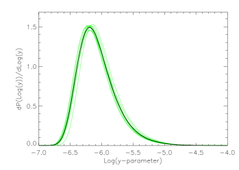
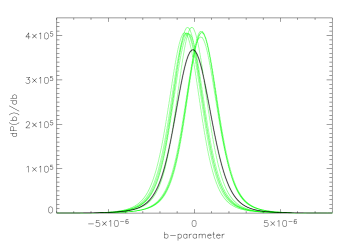
Figure 3: Probability distribution of the logarithm of the $y$-parameter (left panel) and the $b$-parameter (right panel), obtained considering the (1.66 arcsec)² pixels without beam smoothing. The thin lines show the results for 10 different realizations; the thick solid line is the corresponding average.

We also analyse how these statistics change when we smooth our maps to simulate different instrument resolution. We show in the left panel of Fig. 4 the dependence of the distribution of the logarithm of the $y$-parameter: the shape does not change significantly when smoothing the maps down to 0.44 arcmin (corresponding to $16^{2}$ pixels in the original map), while a further reduction of the resolution leads to a change in the shape of the distribution with a resulting absence of the lowest values in the map. On the contrary the probability of obtaining high values remains unchanged also with a beam smoothing of 1.77 arcmin, as a consequence of the fact that the peaks correspond to galaxy clusters which have this typical angular size. At low resolutions the distribution is also more peaked, as it can also be seen in the right panel of Fig. 4: the standard deviation of the distribution drops from 0.3 to less than 0.1 when varying the beam smoothing from 0.2 to 20 arcmin, indicating that in order to capture the main features of the fluctuation field of the tSZ effect a resolution better than $1$ arcmin is desirable.

Figure 4: Left panel: probability distribution functions of the logarithm of the $y$-parameter in the 10 maps for different angular resolutions of the maps. Right panel: standard deviation of the distribution of the logarithm of the $y$-parameter as a function of the beam smoothing.

We show in Fig. 5 the corresponding plots for the distribution of the kSZ effect values. As expected the tails of the distribution function are strongly reduced by the beam smoothing (our results are similar to those obtained by da Silva et al., 2001a). The right panel shows that the standard deviation (solid line) increases at higher resolution due to the fact that, as we will discuss more extensively in Section 5, the kSZ effect has a significant contribution from small-scale signal. The level of non-gaussianity of the distribution can be expressed in terms of the kurtosis $\kappa$ also plotted in the right panel of Fig. 5 (dashed line). The distribution of values is very close to a gaussian (i.e. $\kappa=0$) for resolutions of $\sim$1 arcmin, while at higher resolution the kurtosis increases up to more than 4 thus populating more the tails of distribution. This indicates that the non-gaussianity originated by the kSZ effect must be taken into account when measuring the primordial (i.e. inflationary) non-gaussianity in the CMB signal at scales lower than 1 arcmin.

Figure 5: Left panel: probability distribution functions of the $b$-parameter in the 10 maps for different angular resolutions of the maps. Right panel: standard deviation (solid line) and kurtosis (dashed line) of the distribution of the $b$-parameter as a function of the beam smoothing.

As already mentioned in Section 3.1, unlike the X-ray signal, both the tSZ and the kSZ effects have significant contributions from high-redshift gas. This can be clearly seen in Fig. 6, where we show the contribution to the $y$-parameter and $b$-parameterdivided into equal comoving distance intervals with length of $10h^{-1}$ Mpc (the corresponding redshifts are indicated on the top of the panel). Note that the curves represent the average value of the 10 different light-cone realizations. The tSZ signal (left panel) shows several spikes at low redshift ($z<0.5$), mainly due to the presence of galaxy clusters in the bin. At higher redshifts the distribution is much more regular because the dispersion becomes lower, since the light cones include larger comoving volumes at larger distances. Moreover large collapsed structures are very rare events at $z\ga 2$. Integrating this redshift distribution we obtain, in good agreement with previous analyses (see, e.g., da Silva et al., 2000), that half of the total tSZ signal comes from $z>1$, and only about 20 per cent from $z>2$.

Figure 6: Differential contributions to the $y$-parameter (left panel) and $b$-parameter (right panel) as a function of the comoving distance from the observer; the corresponding redshifts are indicated on the top. The values, representing the mean of the 10 map realizations, are computed in equispaced comoving distance intervals with length of $10\,h^{-1}$ Mpc. The dashed line in the left panel shows the integral of the distribution as a fraction of the final average value of the $y$-parameter.

Since in a given redshift bin there are both gas elements approaching and receding from the observer with similar probabilities, the kSZ signal (right panel), which is the algebraic sum of all the contributions, has a vanishing expectation value. Therefore the distribution plotted in the right panel of Fig. 6 can be considered as a measurement of its dispersion. The plot clearly shows that, even at very high redshift, the contribution to the kSZ effect is non-negligible: as suggested by da Silva et al. (2001a), the increase of the contributing gas mass compensates the decrease of its velocities.

5 The SZ angular power spectra

In order to study the detectability of the SZ effects, it is important to analyze not only the intensity of the signal itself, but also its power at different angular scales. In Fig. 7 we compare the angular power spectra for both SZ effects to the primary CMB one. The displayed SZ spectra, which represent the average of the power spectra of the 10 different light-cone realizations, have been obtained in the approximation of flat sky (which well holds for $\ell>100$) and using a method based on Fast Fourier Transform. We considered a frequency $\nu=30$ GHz for the tSZ effect, that corresponds to $g_{\nu}(x)=-1.94$ (see equation 3), thus near the RJ limit for which the effect is maximum, while the choice of the frequency does not affect the intensity of the kSZ signal (see Section 2). As already discussed in Section 3, both the SZ effects have a significant contribution from high-redshift gas. Since our map-making algorithm replicates the same volume four times at $z>1.4$ (see the comments on Fig. 1), this could introduce a spurious correlation in the power spectrum calculations, therefore, we need to perform some checks to assess the reliability of our results. Our analysis indicates that the kSZ maps are affected by this problem: in fact the kSZ power spectrum computed with this method presents some “fake” peaks at high angular scales generated by gas located at $z>1.4$: for this reason we decided to split each of the 10 kSZ maps into 4 submaps (thus creating 40 different light cones) and to calculate their power spectra separately. We also checked that the tSZ maps are not affected by this problem (e.g. the power spectra calculated with maps and submaps are identical), therefore for the tSZ effect we keep the full maps.

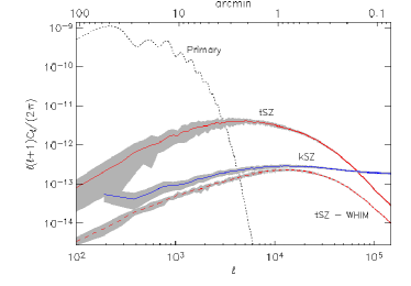
Figure 7: Angular power spectra of the $\Delta T/T_{\rm CMB}$ induced by the different SZ effects as a function of the multipole $\ell$. The dotted line represents the primary CMB signal calculated using cmbfast (Seljak & Zaldarriaga, 1996) and assuming the same cosmological model considered for our hydrodynamical simulation. The solid lines are the tSZ and kSZ power spectra: they represent the average of the power spectra of different maps (10 light-cones for the tSZ effect, 40 for the kSZ one). The dashed line refers to the tSZ power spectrum for the WHIM. The shaded regions represent the r.m.s. calculated between the 10 (40) maps. The tSZ spectra are computed at the frequency $\nu=$ 30 GHz.

Given the size and resolution of our maps, in principle this procedure can allow us to compute the power spectra from $\ell\simeq 95$ ($\ell\simeq 190$ for the kSZ effect) out to $\ell\simeq 7.8\times 10^{5}$. However the finite box size of 192 $h^{-1}$ Mpc of our simulation makes our results reliable only for $\ell\ga 200$ (e.g. the angular extension of 1/2 of the box size at $z=6$). Anyway for the purpose of this paper, we are not interested in investigating the properties of the SZ signal at $\ell\la 1000$, because in this range the primary CMB anisotropies dominate and because at large scales the tSZ signal is highly affected by the local structures (see, e.g. Dolag et al., 2005). For what concerns the small angular scales, our full resolution maps resolve the gravitational softening of the simulation for distances from the observer lower than $\sim 1000\,h^{-1}$ Mpc: therefore, considering also the spatial resolution imposed by the sph code, we can consider our results reliable only for resolutions higher than 3-4 arcsec ($\ell\simeq 2\times 10^{5}$), that subtend distances higher than the gravitational softening for $z\ga 0.17$, from which most of the SZ signals arise, as discussed in Section 4.

The tSZ power spectrum peaks at $\ell\simeq 5000$ and, in the RJ regime, it starts to dominate the primary CMB signal at scales of about 4 arcmin. The kSZ signal is about one order of magnitude lower at these scales. However, it is interesting to note that while at higher $\ell$ the tSZ signal looses power significantly, our model predicts an almost flat kSZ power spectrum, that overcomes the tSZ one for $\ell\ga 7\times 10^{4}$ even in the RJ regime. This behaviour, which is similar to the one obtained by Zhang et al. (2004), is a consequence of both the high contribution from distant, and therefore smaller, objects that affect the kSZ effect signal and of the effect of the galactic winds present in our simulation that are able to increase the power of the signal on very small scales. The tSZ signal arising from the WHIM (also plotted in Fig. 7) peaks at the scales of about 1 arcmin, which roughly corresponds to the angular scales of galaxy groups. Even if the total signal of the WHIM contributes to about 60 per cent of the mean value of the $y$-parameter (as we already noted in Section 4), at the angular scales where the tSZ signal is dominant the amplitude of its power spectrum contributes to less than 10 per cent of the total tSZ one: this shows that the detection of the tSZ signal constitutes a probe almost only for the ICM at temperatures $T>10^{7}$ K, that mainly resides in collapsed structures.

As already noted in Section 2, the intensity of the kSZ effect does not depend on the observed frequency. On the contrary, when increasing the frequency in the RJ regime, the tSZ effect decreases, so the angular scale at which the kSZ signal dominates over the tSZ one becomes higher. Fig. 8 shows the dependence on the angular multipole of the frequency of equality between the power spectra of the two effects. It is worth to note that at 150 GHz the kSZ effect dominates for $\ell\ga 3\times 10^{4}$.

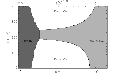
Figure 8: In the $\nu-\ell$ (observed frequency-angular scale) plane we show the regions where the power spectra corresponding to different signals are dominant. Dark shaded, light shaded and white regions show where the primary CMB signal, the kSZ effect and the tSZ effect dominate the other components, respectively. The solid lines show where two effects have the same power, the dashed line corresponds to the frequency of 218 GHz, at which the tSZ signal vanishes.

6 Cross-correlation between the SZ signals

The two SZ signals both depend linearly on the electron density $n_{e}$ and receive the main contribution from the same cosmic structures, so a correlation between the two is expected. However, since temperature and velocity of the gas are not tightly correlated and since the $b$-parameter depends only on the radial component of the velocity, a spread is expected also. This can be seen in the contour plot in Fig. 9 that represents the distribution of pixel values according to the two SZ effects: a significant scatter is present for low ($y\la 10^{-6}$) values of the $y$-parameter to which can correspond $b$-parameter from zero almost to the highest possible values. Anyway, considering the contour levels, most of the surface of the sky is expected to have average values of the two signals.

Figure 9: Distribution of the pixel values for the whole set of 10 maps: the (modulus of the) Doppler $b$-parameter vs. the Compton $y$-parameter. The 6 contour levels enclose 50, 90, 95, 99, 99.5 and 99.9 per cent of the total amount of pixels, respectively.

We show in Fig. 10 the power spectrum of the cross-correlation between the two SZ signals computed at 30 GHz (the scaling with the frequency $\nu$ is simply given by $g_{\nu}(x)$ of equation 3). The correlation peaks at 2 arcmin, the typical scale of galaxy clusters, and a has sharp decrease at higher $\ell$ due to the lack of power of the tSZ effect.

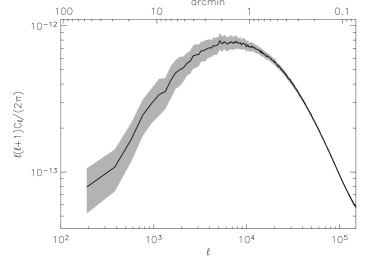
Figure 10: Power spectrum of the cross-correlation tSZ-kSZ at $\nu=30$ GHz as a function of the multipole $\ell$. The solid line represents the average of the power spectra of the 40 submaps; the shaded region shows the corresponding r.m.s.

In order to quantify the strength of the correlation we follow Cheng et al. (2004) and compute the cross-correlation coefficient between the two signals which is defined as

$$r_{\ell}\equiv\frac{C_{\ell}^{\rm tSZ-kSZ}}{\sqrt{C_{\ell}^{\rm tSZ}C_{\ell}^{\rm kSZ}}}\ .$$ (9)

The corresponding results are shown in Fig. 11. Globally the tSZ and kSZ effects present a high correlation ($r_{\ell}\simeq 0.78$), almost independent of the angular scale, indicating that, as already said in the comments on Fig. 9, the average properties of the two signals are similar despite of the different physical dependence. The spread of the correlation in the different light-cones (indicated by the shaded region) is also quite low ($\sim 0.01$); at low $\ell$ it increases ($\sim 0.07$) due to the lack of statistics and the larger cosmic variance.

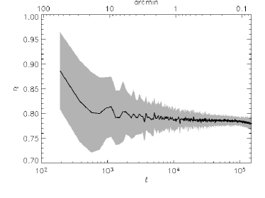
Figure 11: Cross-correlation coefficient between the tSZ and the kSZ effects as a function of the multipole $\ell$. The solid line represents the average of the correlation coefficients of the 40 submaps; the shaded region shows the r.m.s. between them.

7 Cross-correlation with the soft X-ray signal

The ionized gas responsible of the SZ signal also produces an X-ray emission. However, the dependence on both density/scale and redshift is different. Consequently, the cross-correlation between the two signals can provide information on the scales, masses and redshifts contributing to each signal.

The contours in the left panel of Fig. 12 represent the distribution of pixel values according to the soft (0.5–2 keV) X-ray surface brightness (SXRB) and the tSZ effect: it is evident that most of the regions in the sky present both a low soft X-ray emission ($\sim 10^{-14}-10^{-12}$ erg s^-1 cm^-2 deg^-2) and $y$-parameter ($\sim 10^{-6}$), as shown by the distributions reported in Fig. 3. We also notice that, as expected, the amplitudes of the two signals are correlated, even if a significant scatter is present especially for high intensities. Using this bi-dimensional distribution we calculate the maximum-likelihood relation that for a given value of the X-ray surface brightness provides the corresponding one of the $y$-parameter. We proceed in the following way: given $X\equiv\log_{10}($SB(erg s^-1 cm^-2 deg^-2) $)$ and $Y\equiv\log_{10}(y)$, we consider separately the distribution associated to all the different values of $X$ (i.e. the columns of the matrix shown in the left panel of Fig. 12); then for a given $X$ we take the value of $Y$ corresponding to the maximum point of the distribution and its scatter and we fit these data with a polynomial relation given by the formula

$$Y=a_{0}+a_{1}X+a_{2}X^{2}\ ,$$ (10)

where and $a_{i=0,2}$ are the free parameters. We also weight the data according to the total amount of points of each distribution. We obtain the best-fit relation of $Y=-0.72+0.61X+0.015X^{2}$ represented in the plot by the dashed line. Switching the two variables of equation (10) and with the same procedure we obtain also the opposite relation $X=-21-5.8Y-0.73Y^{2}$ shown by the dot-dashed line.

The right panel of Fig. 12 shows the scatter plot between the soft X-ray surface brightness and the (modulus of the) $b$-parameter. The dependence of the kSZ effect from the X-ray emission is weaker than the tSZ effect one, however this plot shows that the highest peaks of the kSZ effect ($|b|>10^{-5}$) are always associated to high surface brightness values (e.g. inner regions of galaxy clusters).

We show in Fig. 13 the power spectrum of the soft (0.5–2 keV) X-ray surface brightness arising from the hot ionized plasma; this power spectrum has been obtained in the same way as described in Section 5 for the tSZ effect, but after dividing the pixel values for their average value corresponding to $4.06\times 10^{-12}$ erg s^-1 cm^-2 deg^-2. The amplitude of the r.m.s. is a direct consequence of the large variance between different fields of the soft X-ray emission coming from the LSS already discussed in Roncarelli et al. (2006a).

Confronting the soft X-ray power spectrum with the one of the tSZ effect shown in Fig. 7 we can see that the former peaks at higher multipoles than the latter. This is due to the fact that the dependence on the square of the gas density of the bremsstrahlung emission makes it more sensitive to the inner parts of collapsed objects.

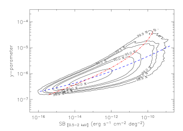
Figure 12: Left panel: distribution of the pixel values for the whole set of 10 maps: the Compton $y$-parameter vs. the soft (0.5–2 keV) X-ray surface brightness. The 6 contour levels enclose 50, 90, 95, 99, 99.5 and 99.9 per cent of the total amount of pixels, respectively. The dashed line represents the maximum-likelihood relation $Y(X)$, obtained by fitting the relation in equation (10); the dot-dashed line represents the opposite maximum-likelihood relation $X(Y)$. Right panel: as the left panel, but for the (modulus of the) Doppler $b$-parameter vs. the soft (0.5–2 keV) X-ray surface brightness.

We show in Fig. 14 the power spectrum of the correlation of the tSZ signal with the soft X-ray emission; again, we computed them following the same methods described in Section 5 (using the set of 40 submaps for the tSZ-kSZ correlation) and assuming the frequency $\nu=30$ GHz. As expected the cross-correlation peaks at an intermediate scale between the two power spectra, and it remains almost constant in the range between $\sim$0.5 and $\sim$3 arcmin. Therefore this constitutes the best angular range to study the two signals together.

Finally, we also compute the cross-correlation coefficient between the SXRB and the two SZ effects and show our results in Fig. 15 (left and right panel, respectively). The correlation with the tSZ signal is as high as $\sim$0.9 at $\ell\sim$1000, slightly decreasing at lower angular scales. This result is in contrast with that obtained by Cheng et al. (2004) that predict a correlation coefficient of about 0.3. The explanation can be found in the different methods used to obtain the results: in fact Cheng et al. (2004) followed an analytical approach using several approximations to account for the cooling of the gas and for the shape of the density profiles. The correlation between the SXRB and the kSZ effect is also very high: in all of our light-cone realizations the values of $r_{\ell}$ for $\ell>$1000 are around 0.8 with negligible differences between them.

8 Conclusions

In this work we have studied the global properties of the tSZ and kSZ effects using the results of a cosmological hydrodynamical simulation of the $\Lambda$CDM model. The simulation (Borgani et al., 2004) follows the evolution of dark matter and baryons accounting for several physical processes that affect the thermodynamical history of the gas: a time dependent photo-ionizing uniform UV background, radiative cooling processes and star formation with consequent feedback processes by SN-II and galactic winds. We used the outputs of the simulations to construct 10 independent light-cone realizations from $z=0$ out to $z=6$ and computed associated mock maps, of size (3.78^∘)², of the Compton $y$-parameter and Doppler $b$-parameter. Using this dataset we estimated the expected statistical properties of the two SZ effects, we calculated their power spectra and studied their cross-correlations. We also analised their correlation properties with the soft (0.5–2 keV) X-ray emission obtained with the same light-cone realizations and already studied in a previous work by Roncarelli et al. (2006a).

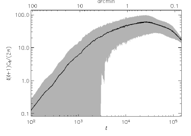
Figure 13: Power spectrum of the SXRB in the soft (0.5–2 keV) X-ray band as a function of the multipole $\ell$: it is obtained after normalizing the pixel values to their average of 4.06 $\times 10^{-12}$ erg s^-1 cm^-2 deg^-2. The solid line represents the average of the power spectra of the 10 maps; the shaded region shows the corresponding r.m.s.

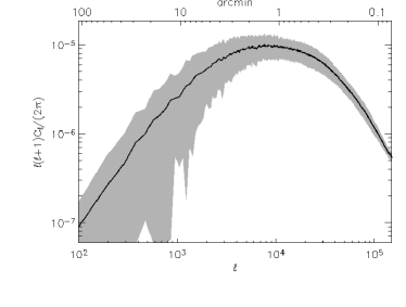
Figure 14: Power spectrum of the cross-correlation SXRB-tSZ at $\nu=30$ GHz as a function of the multipole $\ell$. The solid line represents the average of the power spectra of the 10 maps; the shaded region shows the corresponding r.m.s.

Our main results can be summarized as follows.

1. The mean intensity of the Compton $y$-parameter due to the IGM is $<y>=(1.19\pm 0.32)\times 10^{-6}$: almost 60 per cent of this signal comes from WHIM and about half comes from $z>1$. The distribution of the pixel values in the sky is close to a lognormal, with variance increasing at higher resolution up to 0.3 at the scales of 0.1 arcmin.

2. The peaks of the Doppler $b$-parameter  associated with collapsed objects, are of the order of $|b|\simeq 10^{-5}$. This signal presents a nearly gaussian distribution peaked around 0, with a variance that increases with resolution out to the scales of some arcsecond. The kSZ effect has a significant contribution from high-redshift gas.

   

   

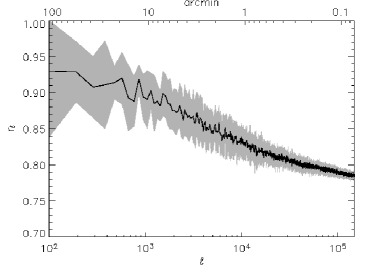
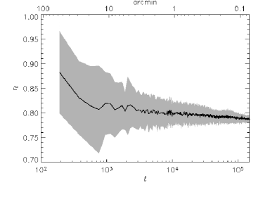
   Figure 15: Cross-correlation coefficient between the SXRB in the (0.5–2 keV) band and the tSZ effect (left panel) and between the SXRB and kSZ effect (right panel) as a function of the multipole $\ell$. The solid line represents the average of the 10 (40) maps; the shaded region shows the r.m.s. between them.

3. The power spectrum analysis shows that the tSZ effect dominates the primary CMB anisotropies for $\ell>3000$ and peaks at $\ell\simeq 5000$. The kSZ signal peaks at $\sim 1$ arcmin and has a flat power spectrum towards high $\ell$ out to $\ell>2\times 10^{5}$. It dominates the tSZ signal for $\ell\ga 7\times 10^{4}$ at all frequencies. The two SZ effect are highly correlated at all scales.

4. The SXRB is highly correlated with the two SZ effects, particularly with the tSZ one ($r_{\ell}\simeq 0.8-0.9$). We also calculated a maximum-likelihood analytic formula that connects the values of the two observables.

In conclusion, our work further demonstrates the importance of the upcoming measurements of both SZ effects and their complementarity with present-day and future X-ray data. A joint analysis of these signals, in combination with high-resolution hydrodynamical simulations, will allow one to obtain insights on the properties of the baryonic component, and on the physical processes acting on it.

References

- Astier et al. (2006) Astier P., et al., 2006, A&A, 447, 31
- Bhattacharya & Kosowsky (2007) Bhattacharya S., Kosowsky A., 2007, ApJ, 659, L83
- Birkinshaw (1999) Birkinshaw M., 1999, Phys. Rep., 310, 97
- Birkinshaw & Hughes (1994) Birkinshaw M., Hughes J. P., 1994, ApJ, 420, 33
- Birkinshaw et al. (1991) Birkinshaw M., Hughes J. P., Arnaud K. A., 1991, ApJ, 379, 466
- Bond et al. (2005) Bond J. R., Contaldi C. R., Pen U.-L., Pogosyan D., Prunet S., Ruetalo M. I., Wadsley J. W., Zhang P., Mason B. S., Myers S. T., Pearson T. J., Readhead A. C. S., Sievers J. L., Udomprasert P. S., 2005, ApJ, 626, 12
- Borgani et al. (2004) Borgani S., et al., 2004, MNRAS, 348, 1078
- Carlstrom et al. (2002) Carlstrom J. E., Holder G. P., Reese E. D., 2002, ARA&A, 40, 643
- Cen & Ostriker (1999) Cen R., Ostriker J. P., 1999, ApJ, 514, 1
- Cheng et al. (2005) Cheng L.-M., et al., 2005, A&A, 431, 405
- Cheng et al. (2004) Cheng L.-M., Wu X.-P., Cooray A., 2004, A&A, 413, 65
- Cole et al. (2005) Cole S., et al., 2005, MNRAS, 362, 505
- Croft et al. (2001) Croft R. A. C., Di Matteo T., Davé R., Hernquist L., Katz N., Fardal M. A., Weinberg D. H., 2001, ApJ, 557, 67
- da Silva et al. (2000) da Silva A. C., Barbosa D., Liddle A. R., Thomas P. A., 2000, MNRAS, 317, 37
- da Silva et al. (2001a) da Silva A. C., Barbosa D., Liddle A. R., Thomas P. A., 2001a, MNRAS, 326, 155
- da Silva et al. (2001b) da Silva A. C., Kay S. T., Liddle A. R., Thomas P. A., Pearce F. R., Barbosa D., 2001b, ApJ, 561, L15
- Davé et al. (2001) Davé R., et al., 2001, ApJ, 552, 473
- Diaferio et al. (2005) Diaferio A., et al., 2005, MNRAS, 356, 1477
- Diego & Majumdar (2004) Diego J. M., Majumdar S., 2004, MNRAS, 352, 993
- Dolag et al. (2005) Dolag K., Hansen F. K., Roncarelli M., Moscardini L., 2005, MNRAS, 363, 29
- Douspis et al. (2006) Douspis M., Aghanim N., Langer M., 2006, A&A, 456, 819
- Eisenstein et al. (2005) Eisenstein D. J., et al., 2005, ApJ, 633, 560
- Ettori et al. (2004) Ettori S., et al., 2004, MNRAS, 354, 111
- Goldstein et al. (2003) Goldstein J. H., Ade P. A. R., Bock J. J., Bond J. R., Cantalupo C., Contaldi C. R., Daub M. D., Holzapfel W. L., Kuo C., Lange A. E., Lueker M., Newcomb M., Peterson J. B., Pogosyan D., Ruhl J. E., Runyan M. C., Torbet E., 2003, ApJ, 599, 773
- Haardt & Madau (1996) Haardt F., Madau P., 1996, ApJ, 461, 20
- Hernández-Monteagudo et al. (2006) Hernández-Monteagudo C., Verde L., Jimenez R., Spergel D. N., 2006, ApJ, 643, 598
- Hetterscheidt et al. (2006) Hetterscheidt M., Simon P., Schirmer M., Hildebrandt H., Schrabback T., Erben T., Schneider P., 2006, preprint, astro-ph/0606571
- Heymans et al. (2005) Heymans C., et al., 2005, MNRAS, 361, 160
- Hoekstra et al. (2006) Hoekstra H., Mellier Y., van Waerbeke L., Semboloni E., Fu L., Hudson M. J., Parker L. C., Tereno I., Benabed K., 2006, ApJ, 647, 116
- Iliev et al. (2007) Iliev I. T., Pen U.-L., Bond J. R., Mellema G., Shapiro P. R., 2007, ApJ, 660, 933
- Massey et al. (2005) Massey R., Refregier A., Bacon D. J., Ellis R., Brown M. L., 2005, MNRAS, 359, 1277
- Mather et al. (1994) Mather J. C., et al., 1994, ApJ, 420, 439
- Monaghan & Lattanzio (1985) Monaghan J. J., Lattanzio J. C., 1985, A&A, 149, 135
- Murante et al. (2004) Murante G., et al., 2004, ApJ, 607, L83
- Parijskij (1973) Parijskij Y. N., 1973, ApJ, 180, L47+
- Rasia et al. (2005) Rasia E., Mazzotta P., Borgani S., Moscardini L., Dolag K., Tormen G., Diaferio A., Murante G., 2005, ApJ, 618, L1
- Rephaeli (1995) Rephaeli Y., 1995, ARA&A, 33, 541
- Rephaeli et al. (2005) Rephaeli Y., Sadeh S., Shimon M., 2005, in Melchiorri F., Rephaeli Y., eds, Background Microwave Radiation and Intracluster Cosmology The Sunyaev-Zeldovich effect. pp 57–+
- Roncarelli et al. (2006a) Roncarelli M., Moscardini L., Tozzi P., Borgani S., Cheng L. M., Diaferio A., Dolag K., Murante G., 2006a, MNRAS, 368, 74
- Roncarelli et al. (2006b) Roncarelli M., Ettori S., Dolag K., Moscardini L., Borgani S., Murante G., 2006b, MNRAS, 373, 1339
- Sadeh & Rephaeli (2004) Sadeh S., Rephaeli Y., 2004, New Astronomy, 9, 373
- Sánchez et al. (2006) Sánchez A. G., Baugh C. M., Percival W. J., Peacock J. A., Padilla N. D., Cole S., Frenk C. S., Norberg P., 2006, MNRAS, 366, 189
- Seljak & Zaldarriaga (1996) Seljak U., Zaldarriaga M., 1996, ApJ, 469, 437
- Semboloni et al. (2006) Semboloni E., et al., 2006, A&A, 452, 51
- Spergel et al. (2003) Spergel D. N., et al., 2003, ApJS, 148, 175
- Spergel et al. (2006) Spergel D. N., et al., 2006, preprint, astro-ph/0603449
- Springel (2005) Springel V., 2005, MNRAS, 364, 1105
- Springel & Hernquist (2003) Springel V., Hernquist L., 2003, MNRAS, 339, 289
- Springel et al. (2001) Springel V., White M., Hernquist L., 2001, ApJ, 549, 681
- Sunyaev & Zel’dovich (1972) Sunyaev R. A., Zel’dovich Y. B., 1972, Comments on Astrophysics and Space Physics, 4, 173
- Sunyaev & Zel’dovich (1980) Sunyaev R. A., Zel’dovich Y. B., 1980, ARA&A, 18, 537
- Tegmark et al. (2006) Tegmark M., et al., 2006, Phys. Rev. D, 74, 123507
- White et al. (2002) White M., Hernquist L., Springel V., 2002, ApJ, 579, 16
- Wood-Vasey et al. (2007) Wood-Vasey W. M., et al., 2007, preprint, astro-ph/0701041
- Zhang et al. (2004) Zhang P., Pen U.-L., Trac H., 2004, MNRAS, 347, 1224
- Zhang et al. (2002) Zhang P., Pen U.-L., Wang B., 2002, ApJ, 577, 555