The Fate of the Universe: Dark Energy Dilution?

Abstract

We study the possibility that dark energy decays in the future and the universe stops accelerating. The fact that the cosmological observations prefer an equation of state of dark energy smaller than -1 can be a signal that dark energy will decay in the future. This conclusion is based in interpreting a $w<-1$ as a signal of dark energy interaction with another fluid. We determine the interaction through the cosmological data and extrapolate it into the future. The resulting energy density for dark energy becomes $\rho_{\phi}=a^{-3(1+w_{\phi})}e^{-\beta(a-1)}$, i.e. it has an exponential suppression for $a\gg a_{o}=1$. In this scenario the universe ends up dominated by this other fluid, which could be matter, and the universe stops accelerating at some time in the near future.

I Introduction

In the last few years the existence of dark energy as a fluid with negative pressure that accelerates the universe at present time has been established DE ,SN . Within the context of field theory and particle physics it is appealing to interpret the dark energy as some kind of particles that interact with the particles of the standard model very weakly. The weakness of the interaction is required since dark energy particles have not been produced in the accelerator and because the dark energy has not decayed into lighter (e.g. massless) fields such as the photon. Perhaps the most appealing candidate for dark energy is that of a scalar field, quintessence Q , which can be either a fundamental particle or a composite particle Qax . It was common to assume the interaction between the dark energy and all other particles to be via gravity only, however recently interacting dark energy models have been proposed IDE -wapp . The interesting effect of this interaction is two fold. On the one hand, the interaction between dark energy and matter, which can be for example dark matter or neutrinos IDE-n , is to give an apparent equation of state of dark energy smaller (more negative) than without the interaction and can be even smaller than -1 wapp , as suggested by the cosmological observations. On the other hand it is also possible to have dark energy interacting with neutrinos and it is tempting to relate both energies since they are of the same order of magnitude IDE-n and a mass of neutrinos larger than $0.8eV$ imply that the dark energy cannot be a cosmological constant IDE-ax .

In general fluids with $w<-1$ give many theoretically problems such as stability issues or wrong kinetic terms as phantom fields ph.etc . However, interacting dark energy is a very simple and attractive option which we will use in this letter.

Since the dark energy dilutes slower than matter we expect it to dominate the universe at late times. So, once the universe begins to accelerate due to dark energy we expect it to maintain this state of acceleration in the future and the universe will end up completely dominated by dark energy. In this letter we would like to study if this fate of the universe is unavoidable or we could have a transition from an accelerating universe to a non accelerating one in which the dark energy decays into another fluid. We will show that the fact that the cosmological data DE , specially the SN1a data SN , prefer an equation of state $w$ of dark energy smaller than minus one can be a signal that dark energy will decay in the future and the universe will stop accelerating. This conclusion is based in interpreting a $w<-1$ as a signal of dark energy interaction with another fluid. We determine the interaction through the cosmological observations and extrapolating it into the future.

This letter is organized as follows. In section II we present the generic evolution of two interacting fluids. In section III we introduce the effective and apparent equations of state and in section IV we give the evidence a dark energy decay. Finally we present our conclusions.

II Interacting Dark Energy

II.1 Fluid Evolution

The evolution of two interacting fluids $\rho_{\phi}$ and $\rho_{b}$, which can be quintessence scalar field $\phi$ for dark energy ”DE” and another fluid ($\rho_{b}$), as for example matter or radiation, is given by

$$\dot{\rho}_{\phi} = -3H\rho_{\phi}(1+w_{\phi})-\delta(t)$$ (1)

$$\dot{\rho}_{b} = -3H\rho_{b}(1+w_{b})+\delta(t)$$ (2)

with $H=\dot{a}/a$ the Hubble parameter and $\delta(t)$ the interaction coupling. This $\delta$ is a dissipative term, it depends on the interaction term between the particles of $\rho_{\phi}$ and $\rho_{b}$ and is in general a function of time. The equation of state parameters $w_{\phi}\equiv p_{\phi}/\rho_{\phi}$ and $w_{b}\equiv p_{b}/\rho_{b}$ may be functions of time. Without lack of generality we will take $w_{b}>w_{\phi}$, which is consistent with assuming $\rho_{\phi}$ as the dark energy in the absence of an interaction term.

A simple general solution for $\rho_{b}$ can be obtained by taking $w_{b}$ constant and $\delta=A(t)\rho_{b}$. Eq.(2) becomes $\dot{\rho}_{b}=-[3H(1+w_{\phi})-A]\rho_{b}$ and it has a solution

$$\rho_{b}=\rho_{bo}a^{-3(1+w_{b})}\,e^{\int_{to}^{t}dtA}=\widetilde{\rho_{b}}\,e^{\int_{to}^{t}dtA}$$ (3)

with $\widetilde{\rho_{b}}\equiv\rho_{bo}a^{-3(1+w_{b})}$, the evolution of $\rho_{b}$ without an interacting term, i.e. $\delta=0$. We take $a(t_{o})\equiv a_{o}=1$ at present time. A similar solution can be obtained for $\rho_{\phi}$ with $w_{\phi}$ constant and setting $\delta=\widetilde{A}\rho_{\phi}$ the solution to eq.(1) gives

$$\rho_{\phi}=\rho_{\phi o}a^{-3(1+w_{\phi})}\,e^{-\int_{to}^{t}dt\widetilde{A}}=\widetilde{\rho}_{\phi}\,e^{-\int_{to}^{t}dt\widetilde{A}}$$ (4)

with $\widetilde{\rho}_{\phi}\equiv\rho_{\phi o}a^{-3(1+w_{\phi})}$ the evolution for $\delta=0$. Of course $A,\widetilde{A}$ are related by $\delta=\widetilde{A}\rho_{\phi}=A\rho_{b}$. Clearly the sign of $A$, i.e. $\delta$, determines whether $\rho_{\phi}$ and $\rho_{b}$ will evolve faster or slower with the interaction term than without it. So, for $A$ positive $\rho_{b}$ will dilute slower while for $A$ negative it will dilute faster.

If we take the ratio $y\equiv\rho_{\phi}/\rho_{b}=\Omega_{\phi}/\Omega_{b}$ from eqs.(3) and (4) we have

$$y=\frac{\rho_{\phi}}{\rho_{b}}=y_{o}a^{3(w_{b}-w_{\phi})}\,e^{-\int_{to}^{t}dtA(1+1/y)}$$ (5)

with $y_{o}=\rho_{\phi o}/\rho_{bo}$, and taking the derivative of $y$ w.r.t. time we find

$$\dot{y}=3Hy\left[\Delta w-\Upsilon\right]$$ (6)

with $\Delta w\equiv w_{b}-w_{\phi}$ and

$$\Upsilon\equiv\frac{\delta}{3H}\left(\frac{\rho_{\phi}+\rho_{b}}{\rho_{\phi}\rho_{b}}\right)=\frac{A(1+y)}{3Hy}.$$ (7)

The value for $y$ is constraint to $0\leq y\leq\infty$ with $y=0$ for $\rho_{\phi}=0$ and $y=\infty$ for $\rho_{b}=0$. Clearly from eq.(6) we see that the evolution of $y$ depends on the sign of $\Delta w-\Upsilon$.

II.1.1 Non Interaction solution: $\Delta w>\Upsilon$

If $(w_{b}-w_{\phi})>\Upsilon$ then $\dot{y}$ is positive and $y$ will increase, i.e. $\rho_{b}$ will dilute faster than $\rho_{\phi}$, and we will end up with $\rho_{\phi}$ dominating the universe. In this case the interaction term $\delta$ is subdominant and the evolution of $\rho_{\phi}$ and $\rho_{b}$ is the usual one, i.e. $\rho_{\phi}\propto a^{-3(1+w_{\phi})}$ and $\rho_{b}\propto a^{-3(1+w_{b})}$.

II.1.2 Interacting solution: $\Delta w<\Upsilon$

For $\rho_{b}$ to dominate the universe we need $y\ll 1$ at late time and the (interaction) term $\Upsilon$ should dominate over $\Delta w$. A simple example is when $\widetilde{A}$ is constant and positive. In this case eq.(5) is

$$y=y_{i}\left(\frac{a}{a_{i}}\right)^{3(w_{b}-w_{\phi})}\,e^{-\widetilde{A}t}\rightarrow 0$$ (8)

at late times for any value of $w_{b}-w_{\phi}$.

II.1.3 Finite solution: $\Delta w=\Upsilon$

A solution to eq.(6) with $y$ constant and $\rho_{b}\neq 0,\rho_{\phi}\neq 0$ is only possible if $A/H$ (or $\widetilde{A}/H$) is positive and constant since $\Upsilon=A(1+y)/3Hy=\widetilde{A}(1+y)/3H=\Delta w$ must be constant and positive, taking $w_{b}-w_{\phi}>0$ constant. Let us take $\widetilde{A}/H=C>0$ constant, i.e. with $\delta=\widetilde{A}\rho_{\phi}=CH\rho_{\phi}$, and from $\dot{y}=0$, i.e. $\Upsilon=\widetilde{A}(1+y)/3H=\Delta w$, we get a stable value of $y$ given by

$$y_{s}=\frac{\Omega_{\phi}}{\Omega_{b}}=\frac{H}{\widetilde{A}}\;3(w_{b}-w_{\phi})-1=\frac{3(w_{b}-w_{\phi})}{C}-1.$$ (9)

It is easy to see that the solution $y_{s}$ is stable since from eq.(6) the fluctuation $\delta y=y-y_{s}$ to first order behaves as $\delta\dot{y}/\delta y=-\widetilde{A}y_{s}$ ($\widetilde{A}$ is positive by hypothesis) giving $\delta y\rightarrow 0$. Furthermore, since $\widetilde{A}$ is proportional to $H=\dot{a}/a$ then we can integrate eq.(4) with $\widetilde{A}dt=[3(w_{b}-w_{\phi})/(1+y_{s})]Hdt=CHdt=Cda/a$ to give

$$\rho_{\phi}=\rho_{\phi i}\left(\frac{a}{a_{i}}\right)^{-3(1+w_{\phi})-C}=\rho_{\phi i}\left(\frac{a}{a_{i}}\right)^{-3(1+\frac{w_{b}+y_{s}w_{\phi}}{1+y_{s}})}$$ (10)

where we have used that $C=3(w_{b}-w_{\phi})/(1+y_{s})$. Since $C$ is positive the solution in eq.(10) dilutes faster than the non interacting solution $\rho_{\phi}\propto a^{-3(1+w_{\phi})}$ and with an effective equation of state $w_{eff}=w_{\phi}+C/3=(w_{b}+y_{s}w_{\phi})/(1+y_{s})>w_{\phi}$.

III Effective and Apparent Equation of State

We will now introduce the effective eq. of state $w_{eff}$ and the apparent eq. of state $w_{app}$.

III.1 Effective Equation of State

To obtain an effective equation of state we simply rewrite eqs.(1) and (2) as

$$\dot{\rho}_{\phi} = -3H\rho_{\phi}(1+w_{eff})$$

$$\dot{\rho}_{b} = -3H\rho_{b}(1+w_{beff})$$ (11)

with the effective equation of state defined by

$$w_{eff}=w_{\phi}+\frac{\delta}{3H\rho_{\phi}},\hskip 28.45274ptw_{beff}=w_{b}-\frac{\delta}{3H\rho_{b}}.$$ (12)

The solution to eq.(III.1) is

$$\rho_{\phi} = e^{-3\int_{to}^{t}(1+w_{eff})da/a}=a^{-3(1+w_{\phi})}\,e^{-\int_{to}^{t}\frac{\delta}{\rho_{\phi}}dt}$$

$$\rho_{b} = e^{-3\int_{to}^{t}(1+w_{beff})da/a}=a^{-3(1+w_{b})}\,e^{\int_{to}^{t}\frac{\delta}{\rho_{b}}dt}$$ (13)

where we have assumed in the second equality of eqs.(III.1) that $w_{\phi},w_{b}$ are constant. We see from eqs.(III.1) that $w_{eff},w_{beff}$ give the complete evolution of $\rho_{\phi}$ and $\rho_{b}$. For $\delta>0$ we have $w_{eff}>w_{\phi}$ and the fluid $\rho_{\phi}$ will dilute faster then without the interaction term (i.e. $\delta=0$) while $\rho_{b}$ will dilute slower since $w_{beff}<w_{b}$. Which fluid dominates at late time will depend on which effective equation of state is smaller. The difference in eqs.(12) is

$$\Delta w_{eff}\equiv w_{beff}-w_{eff}=\Delta w-\Upsilon$$ (14)

with $\Upsilon$ defined in eq.(7) while the sum gives

$$\Omega_{b}w_{beff}+\Omega_{\phi}w_{eff}=\Omega_{b}w_{b}+\Omega_{\phi}w_{\phi}.$$ (15)

Clearly the relevant quantity to determine the relative growth is given by $\Upsilon$ and if $\Upsilon>\Delta w$ we have $\Delta w_{eff}<0$ and $\rho_{b}$ will dominate the universe at late times while for $\Upsilon<\Delta w$ we have $\Delta w_{eff}>0$ and $\rho_{\phi}$ will prevail. For no interaction $\delta=0$ and $\Upsilon=0$ giving $\Delta w_{eff}=\Delta w>0$ and $\rho_{\phi}$ dominates at late times. If $\Upsilon=\Delta w$ then $w_{beff}=w_{eff}$ and the ratio of both fluids $\rho_{b}/\rho_{\phi}$ will approach a constant value, and if the universe is dominated by $\rho_{\phi}+\rho_{b}$, i.e. $\Omega_{\phi}+\Omega_{b}=1$, then eq.(15) gives

$$w_{\phi}\leq\;w_{eff}=w_{b}\Omega_{b}+w_{\phi}(1-\Omega_{b})\;\leq w_{b},$$ (16)

i.e. the effective equation of state is constraint between $w_{\phi}$ and $w_{b}$. Of course eqs.(14) and (7) are consistent with the analysis of eq.(6).

III.2 Apparent Equation of State

An interesting result of the interaction between dark energy with other particles is to change the apparent equation of state of dark energy IDE -wapp . An observer that supposes that DE has no interaction sees a different evolution of DE as an observer that takes into account for the interaction between DE and another fluid. This effect allows to have an apparent equation of state $w<-1$ for the “non-interaction” DE wapp even though the true equation of state of DE is larger than -1.

Let as take the energy density $\rho=\rho_{\phi}+\rho_{b}=\rho_{DE}+\widetilde{\rho_{b}}$. The energy densities $\rho_{\phi},\rho_{b}$ are given by eqs.(1) and (2) and these two fluid interact via the $\delta$ term. On the other hand the energy densities $\rho_{DE}$ and $\widetilde{\rho_{b}}$ do not interact with each other by hypothesis and therefore we have $\dot{\widetilde{\rho_{b}}}=-3H(1+w_{b})$ and $\dot{\rho}_{DE}=-3H\rho_{DE}(1+w_{ap})$, i.e.

$$\widetilde{\rho_{b}} = \rho_{bo}a^{-3(1+w_{b})}$$

$$\rho_{DE} = \rho_{DEo}a^{-3(1+w_{ap})}$$ (17)

if $w_{b},w_{app}$ are constant. It was pointed out that the apparent equation of state $w_{app}$ can take values smaller than -1 and it is given by wapp

$$w_{ap} = \frac{w_{\phi}}{1-x}$$ (18)

$$x\equiv-\frac{\widetilde{\rho_{b}}}{\rho_{\phi}}\left(\frac{\rho_{b}}{\widetilde{\rho_{b}}}-1\right) = -\frac{\rho_{bo}a^{-3}}{\rho_{\phi}}\left(e^{\int_{to}^{t}dtA}-1\right)$$

valid if $w_{b}=0$ and we have used eq.(3). We see from eq.(18) that for $\rho_{b}<\widetilde{\rho_{b}}$, i.e. $A>0$ (or $\delta>0$), we have $x>0$ and $w_{ap}<w_{\phi}$ for $t<t_{o}$ which allows to have a $w_{ap}$ smaller than -1.

The result in eq.(18) can be generalized to the interaction between two arbitrary fluids. Taking the time derivative of $\rho=\rho_{\phi}+\rho_{b}$ and using eqs.(1) and (2), for an arbitrary interacting term $\delta$, we get $\dot{\rho}_{DE}=-3H\rho_{DE}(1+w_{ap})$ with

$$w_{ap}=\frac{w_{\phi}-w_{b}x}{1-x}$$ (19)

with

$$x\equiv-\frac{\widetilde{\rho_{b}}}{\rho_{\phi}}\left(\frac{\rho_{b}}{\widetilde{\rho_{b}}}-1\right)=-\frac{\rho_{bo}a^{-3(1+w_{b})}}{\rho_{\phi}}\left(e^{\int_{to}^{t}dtA}-1\right)$$ (20)

where we have used eq.(3). Of course $w_{ap},\,x$ in eq.(19) reduce for $w_{b}=0$ to $w_{ap},\,x$ as given in eq.(18). For $t=t_{o}$ we have $x=0$ and if there is no interaction $\delta=A=0$ we have $\rho_{b}=\widetilde{\rho_{b}}$, $x=0$ and $w_{ap}=w_{\phi}$. An apparent equation of state $w_{ap}<w_{\phi}$ is given for $0<x\Delta w=x(w_{b}-w_{\phi})$, i.e. $x>0$. A positive $x$ needs $\widetilde{\rho_{b}}<\rho_{b}$ which from eq.(3) implies a positive interaction term $\delta=A\rho_{b}$. We also see that a positive $w_{b}$ gives a more negative $w_{ap}$ than for $w_{b}=0$.

It is interesting to note, see table 1 that the apparent equation of state $w_{app}$ is smaller than $w_{\phi}$ for a positive $\delta$ while the effective equation of state $w_{eff}$ is in this case larger than $w_{\phi}$. This clearly shows that the apparent equation of state is an ”optical” effect not a true evolution.

$\delta(t)$	$w_{eff},\forall a$	$w_{app}(a<a_{o})$	$w_{app}(a>a_{o})$
$\delta>0$	$w_{eff}>w_{\phi}$	$w_{app}<w_{\phi}$	$w_{app}>w_{\phi}$
$\delta<0$	$w_{eff}<w_{\phi}$	$w_{app}>w_{\phi}$	$w_{app}<w_{\phi}$

Table 1: We show the different relative sizes of $w_{app}$ and $w_{eff}$ with respect to $w_{\phi}$ as a function of the sign of the interaction term $\delta(t)$.

IV Evidence for Dark Energy Decay

The SN1a observations prefer an equation of state $w<-1$ for dark energy. In principal a $w<-1$ for a fluid is troublesome since it has instabilities and causality problems. However, as seen in section III this can be an optical effect due to the interaction between dark energy with other particles as for example dark matter or neutrinos.

Here, we will assume that $w<-1$ due to this interaction and we will show that this can be interpreted as a signal for a dark energy decay in the future with the universe no longer accelerating.

The complete evolution of dark energy is given by the effective equation of state $w_{eff}$ given by eq.(12) while the observed equation of state, if we assume no interaction, is given by eq.(18), i.e. $w_{app}=w_{\phi}/(1-x)$.

For values of the scale factor $a$ close to present day $a_{o}=1$ we propose to approximate $x$ linearly by

$$x=\beta(a_{o}-a)=-\beta\delta a$$ (21)

with $\beta$ a constant to be determined by observations and $\delta a\equiv a-a_{o}$. A positive $x$ in the past (i.e. $a<a_{o}$) requires $\beta>0$. Eq.(21) satisfies the requirements $x(a_{o})=0$ and we have for $w_{app}>w_{\phi}$, $x<0$ for $a>a_{o}$.

The SN1a data are in the range $1>a>2/5$, i.e. for a redshift $0<z<1.5$, and the best fit solution has an average equation of state $<w>\approx-1.1$ DE . Taking the average of $w_{app}=w_{\phi}/(1-x)$ we have

$$<w_{app}>\equiv\frac{\int_{a_{1}}^{a_{o}}w_{app}\,da}{\int_{a_{1}}^{a_{o}}da}=\frac{w_{\phi}Log\left[1-\beta(1-a_{1})\right]}{\beta(a_{1}-1)}$$ (22)

where we have used eq.(21) and $a_{o}=1$. As an example let as take $<w_{app}>=-1.1$, as suggested by the observations SN ,IDE-ax , and $w_{\phi}=-0.9,w_{b}=0,\;a_{1}=2/5$. In this case we obtained from eq.(22) the value $\beta=0.56$. If instead of taking the average as in eq.(22) we simple take the $w_{app}$ evaluated at the extreme points we have $<w_{app}>=\frac{1}{2}(w_{app}(a_{o})+w_{app}(a_{1}))$ giving the simple analytic expression $\beta=\frac{2<w_{app}>-2w_{\phi}}{(1-a_{1})(2<w_{app}>-w_{\phi})}$ and for our previous example we find $\beta=0.51$. The difference in determining $\beta$ is small and the expression for $\beta$ becomes analytic as a function of $<w_{app}>$.

Now, we would like to determine the effective (true) eq. of state for dark energy. From eq.(18) we have

$$x=-\frac{\rho_{b}}{\rho_{\phi}}\left(1-e^{-\int_{to}^{t}dtA}\right)\simeq-\frac{\rho_{b}}{\rho_{\phi}}A\delta t$$ (23)

where we have approximated $e^{\int_{to}^{t}dtA}\simeq 1-A\delta t$ and $\delta t\equiv t-t_{o}$. Taking $\delta=A\rho_{b}$ and eq.(23) we have $\delta=-x\rho_{\phi}/\delta t$ and using $\delta t=\delta a/aH$ and eq.(21) we get an interaction term

$$\delta=a\beta H\rho_{\phi}.$$ (24)

Eq.(12) becomes then

$$w_{eff}=w_{\phi}+\frac{\delta}{3H\rho_{\phi}}\simeq w_{\phi}+\frac{a\beta}{3}$$ (25)

and the effective equation of state for the b-fluid gives

$$w_{beff}=w_{b}-\frac{\delta}{3H\rho_{b}}\simeq w_{b}-\frac{a\beta}{3}\frac{\Omega_{\phi}}{\Omega_{b}}.$$ (26)

Using eq.(4) or equivalently eq.(III.1) with the interaction term given in eq.(24) we get an energy density

$$\rho_{\phi}=a^{-3(1+w_{\phi})}e^{-\beta(a-1)}$$ (27)

which shows that $\rho_{\phi}$ dilutes as $a^{-3(1+w_{\phi})}$ for $a\ll a_{o}=1$ and $\rho_{\phi}$ is exponentially suppressed for $a\gg 1$. From eqs.(25) and (26) we find that $w_{beff}<w_{eff}$ for $a>a_{*}\equiv 3\Delta w\Omega_{\phi}/\beta$ (taking $\Omega_{\phi}+\Omega_{b}=1$), i.e. for $a>a_{*}$ dark energy dilutes faster than the b-fluid.

For our previous example with $w_{\phi}=-0.9,w_{b}=0,\beta=0.56$ and present day values $\Omega_{\phi o}=0.7$ and $\Omega_{bo}=0.3$, we find $w_{eff}=w_{beff}$ at $a_{*}\simeq 1.3$. Furthermore $w_{eff}=0$ at $a=-3w_{\phi}/\beta=4.8$, i.e. due to the interaction $w_{eff}$ grows from $w_{eff}=-0.9$ to $w_{eff}=0$. In this case the universe goes from a decelerating to an accelerating epoch and back to a decelerating one at a scale factor $a_{d}=5.1$.

From eq.(26) with $w_{b}=0$ we have $w_{beff}\leq 0$. Since $w_{beff}<w_{eff}$ for $\Omega_{\phi}\neq 0$ and $a>a_{*}$ then we will have at late times $\Omega_{\phi}\rightarrow 0$ and $w_{beff}\rightarrow 0$ with a universe completely dominated by the fluid $\rho_{b}$, matter in this case, and decelerating.

We show in fig.1 the evolution of $\Omega_{\phi},\Omega_{b}$ in the example with an interaction term $\delta=-x\rho_{\phi}/\delta t=-a\beta H\rho_{\phi}$ with $x$ given by eq.(21) and $w_{\phi}=-0.9$ and $\beta=0.56$, such that the average $<w_{app}>=-1.1$. Notice that for $a<1$ the dark energy grows relative to the b-fluid while for $a>1$ (i.e. in the future) the b-fluid dominates. In fig.2 we show the effective equations of state given by eqs.(25) and (26) and both are larger than -1 at all times. In fig.3 we show the apparent eq. of state (c.f. eq.(18)) where $w_{app}$ is smaller than $w_{\phi}$ for $a<1$ as suggested by the SN1a data but it becomes larger than $w_{\phi}$ for $a>1$.

Figure 1: We show the energy densities $\Omega_{\phi},\Omega_{b}$ (red (dotted) and blue (solid) respectively) as a function of the scale factor $a$. The $b$-fluid dominates at late time. The vertical line is present time $a=1$.

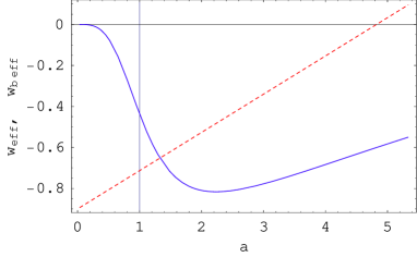
Figure 2: We show the effective eqs. of state $w_{eff},w_{beff}$ (red (dotted) and blue (solid) respectively) as a function of the scale factor $a$. The vertical line is present time $a=1$.

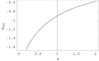
Figure 3: We show the apparent eq. of state $w_{app}$ as a function of the scale factor $a$. It is less than -1 for $a<a_{0}=1$. The vertical line is present time $a=1$.

V Conclusions

The cosmological observations prefer an equation of state $w<-1$ for dark energy. We obtain an apparent equation of state for dark energy smaller than minus one due to the interaction between dark energy and another fluid (b-fluid). Form the observational data we determine the interaction term, close to present day, and we show that this interaction imply that dark energy will dilute faster than the b-fluid. The interaction term is $\delta=a\beta H\rho_{\phi}$ which gives an energy density $\rho_{\phi}=a^{-3(1+w_{\phi})}e^{-\beta(a-1)}$, it has an exponential suppression for $a\gg a_{o}$. The resulting universe is a decelerating universe dominated by the b-fluid, which could be dark matter.

- (1)
- (2) D. N. Spergel et al., astro-ph/0603449; M. Tegmark et al. Phys.Rev.D74:123507,2006; U. Seljak, A. Slosar and P. McDonald,JCAP 0610:014,2006
- (3) A. G. Riess et al. [Supernova Search Team Collaboration], Astrophys. J. 607, 665 (2004); W. M. Wood-Vasey et al., arXiv:astro-ph/0701041; N. Palanque-Delabrouille [SNLS Collaboration], arXiv:astro-ph/0509425.
- (4) I. Zlatev, L. Wang and P.J. Steinhardt, Phys. Rev. Lett.82 (1999) 896; Phys. Rev. D59 (1999)123504; A. de la Macorra, G. Piccinelli Phys.Rev.D61:(2002)123503
- (5) P. Binetruy, Phys.Rev. D60 (1999) 063502, Int. J.Theor. Phys.39 (2000) 1859; A. de la Macorra, C. Stephan-Otto, Phys.Rev.Lett.87:(2001) 271301; A. De la Macorra JHEP01(2003)033; A. de la Macorra, Phys.Rev.D72:043508,2005
- (6) L. Amendola, Phys. Rev. D 62, 043511 (2000); M. Kaplinghat and A. Rajaraman, arXiv:astro-ph/0601517. D. B. Kaplan, A. E. Nelson and N. Weiner, Phys. Rev. Lett. 93, 091801 (2004) R. D. Peccei, Phys. Rev. D 71, 023527 (2005) A. W. Brookfield, C. van de Bruck, D. F. Mota and D. Tocchini-Valentini, Phys.Rev.D 73 (2006) 083515; M. Kaplinghat and A. Rajaraman, arXiv:astro-ph/0601517.
- (7) S. Das, P. S. Corasaniti and J. Khoury,Phys. Rev. D 73, 083509 (2006)
- (8) D. B. Kaplan, A. E. Nelson and N. Weiner, Phys. Rev. Lett. 93, 091801 (2004) R. D. Peccei, Phys. Rev. D 71, 023527 (2005) A. W. Brookfield, C. van de Bruck, D. F. Mota and D. Tocchini-Valentini, Phys.Rev.D 73 (2006) 083515;
- (9) A. de la Macorra, A. Melchiorri, P. Serra, R. Bean astro-ph/0608351 (to be publsihed in Astrop.Phys.)
- (10) S. Das, P. S. Corasaniti and J. Khoury,Phys. Rev. D 73, 083509 (2006)
- (11) S. M. Carroll, M. Hoffman and M. Trodden, Phys. Rev. D 68, 023509 (2003); A. de la Macorra, H. Vucetich, JCAP09(2004)012