ARE RADIO SOURCES AND GAMMA RAY BURSTS LUMINAL BOOMS?

Abstract

The softening of a Gamma Ray Burst (GRB) afterglow bears remarkable similarities to the frequency evolution in a sonic boom. At the front end of the sonic boom cone, the frequency is infinite, much like a GRB. Inside the cone, the frequency rapidly decreases to infrasonic ranges and the sound source appears at two places at the same time, mimicking the double-lobed radio sources. Although a “luminal” boom violates the Lorentz invariance and is therefore forbidden, it is tempting to work out the details and compare them with existing data. This temptation is further enhanced by the observed superluminality in the celestial objects associated with radio sources and some GRBs. In this article, we calculate the temporal and spatial variation of observed frequencies from a hypothetical luminal boom and show remarkable similarity between our calculations and current observations.

Managing Editor

1 Introduction

A sonic boom is created when an object emitting sound passes through the medium faster than the speed of sound in that medium. As the object traverses the medium, the sound it emits creates a conical wavefront, as shown in Fig. 1. The sound frequency at this wavefront is infinite because of the Doppler shift. The frequency behind the conical wavefront drops dramatically and soon reaches the infrasonic range. This frequency evolution is remarkably similar to afterglow evolution of a gamma ray burst (GRB).

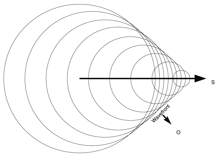
Figure 1: The frequency evolution of sound waves as a result of the Doppler effect in supersonic motion. The supersonic object S is moving along the arrow. The sound waves are “inverted” due to the motion, so that the waves emitted at two different points in the trajectory merge and reach the observer (at O) at the same time. When the wavefront hits the observer, the frequency is infinity. After that, the frequency rapidly decreases.

Gamma Ray Bursts are very brief, but intense flashes of $\gamma$ rays in the sky, lasting from a few milliseconds to several minutes,[1] and are currently believed to emanate from cataclysmic stellar collapses. The short flashes (the prompt emissions) are followed by an afterglow of progressively softer energies. Thus, the initial $\gamma$ rays are promptly replaced by X-rays, light and even radio frequency waves. This softening of the spectrum has been known for quite some time,[2] and was first described using a hypernova (fireball) model. In this model, a relativistically expanding fireball produces the $\gamma$ emission, and the spectrum softens as the fireball cools down.[3] The model calculates the energy released in the $\gamma$ region as $10^{53}$–$10^{54}$ ergs in a few seconds. This energy output is similar to about 1000 times the total energy released by the sun over its entire lifetime.

More recently, an inverse decay of the peak energy with varying time constant has been used to empirically fit the observed time evolution of the peak energy[4, 5] using a collapsar model. According to this model, GRBs are produced when the energy of highly relativistic flows in stellar collapses are dissipated, with the resulting radiation jets angled properly with respect to our line of sight. The collapsar model estimates a lower energy output because the energy release is not isotropic, but concentrated along the jets. However, the rate of the collapsar events has to be corrected for the fraction of the solid angle within which the radiation jets can appear as GRBs. GRBs are observed roughly at the rate of once a day. Thus, the expected rate of the cataclysmic events powering the GRBs is of the order of $10^{4}$–$10^{6}$ per day. Because of this inverse relationship between the rate and the estimated energy output, the total energy released per observed GRB remains the same.

If we think of a GRB as an effect similar to the sonic boom in supersonic motion, the assumed cataclysmic energy requirement becomes superfluous. Another feature of our perception of supersonic object is that we hear the sound source at two different location as the same time, as illustrated in Fig. 2. This curious effect takes place because the sound waves emitted at two different points in the trajectory of the supersonic object reach the observer at the same instant in time. The end result of this effect is the perception of a symmetrically receding pair of sound sources, which, in the luminal world, is a good description of symmetric radio sources (Double Radio source Associated with Galactic Nucleus or DRAGN).

Figure 2: The object is flying from $A^{\prime}$ to $A$ through $B^{\prime}$ and $B$ at a constant supersonic speed. Imagine that the object emits sound during its travel. The sound emitted at the point $B^{\prime}$ (which is near the point of closest approach $B$) reaches the observer at $O$ before the sound emitted earlier at $A^{\prime}$. The instant when the sound at an earlier point $A^{\prime}$ reaches the observer, the sound emitted at a much later point $A$ also reaches $O$. So, the sound emitted at $A$ and $A^{\prime}$ reaches the observer at the same time, giving the impression that the object is at these two points at the same time. In other words, the observer hears two objects moving away from $B^{\prime}$ rather than one real object.

Radio Sources are typically symmetric and seem associated with galactic cores, currently considered manifestations of space-time singularities or neutron stars. Different classes of such objects associated with Active Galactic Nuclei (AGN) were found in the last fifty years. Fig. 3 shows the radio galaxy Cygnus A,[6] an example of such a radio source and one of the brightest radio objects. Many of its features are common to most extragalactic radio sources: the symmetric double lobes, an indication of a core, an appearance of jets feeding the lobes and the hotspots. Refs. hotspot1 and hotspot2 have reported more detailed kinematical features, such as the proper motion of the hotspots in the lobes.

Symmetric radio sources (galactic or extragalactic) and GRBs may appear to be completely distinct phenomena. However, their cores show a similar time evolution in the peak energy, but with vastly different time constants. The spectra of GRBs rapidly evolve from $\gamma$ region to an optical or even RF afterglow, similar to the spectral evolution of the hotspots of a radio source as they move from the core to the lobes. Other similarities have begun to attract attention in the recent years.[9]

This article explores the similarities between a hypothetical “luminal” boom and these two astrophysical phenomena, although such a luminal boom is forbidden by the Lorentz invariance. Treating GRB as a manifestation of a hypothetical luminal boom results in a model that unifies these two phenomena and makes detailed predictions of their kinematics.

2 Symmetric Radio Sources

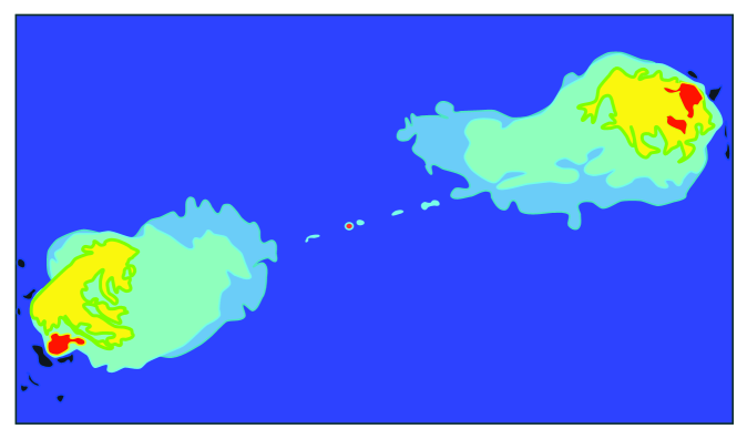
Figure 3: The radio jet and lobes in the hyperluminous radio galaxy Cygnus A. The hotspots in the two lobes, the core region and the jets are clearly visible. (Reproduced from an image courtesy of NRAO/AUI.)

Here, we show that our perception of a hypothetical object crossing our field of vision at a constant superluminal speed is remarkably similar to a pair of symmetric hotspots departing from a fixed point with a decelerating rate of angular separation.

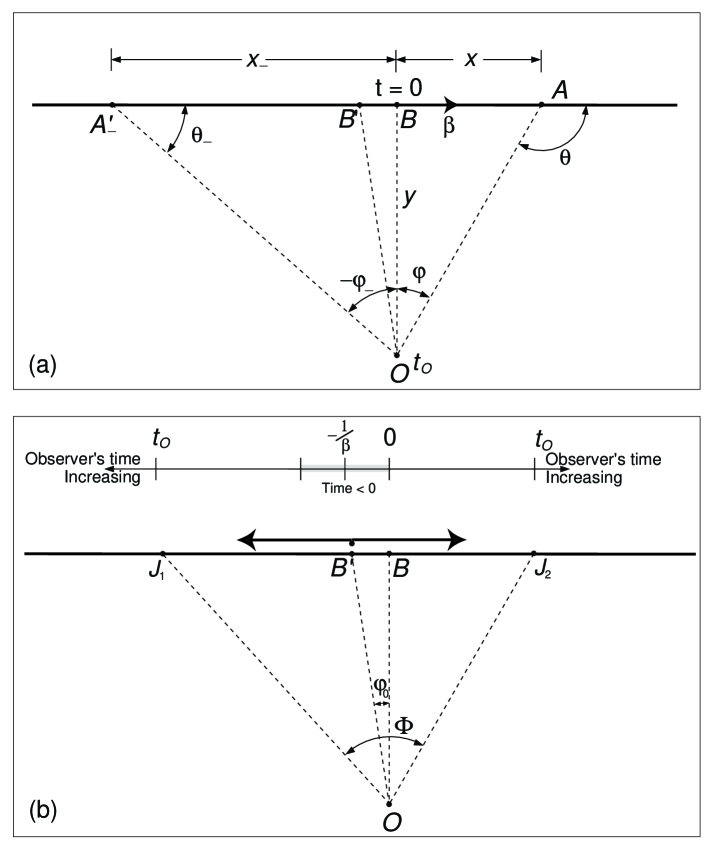
Figure 4: The top panel (a) shows an object flying along $A_{-}^{\prime}BA$ at a constant superluminal speed. The observer is at $O$. The object crosses $B$ (the point of closest approach to $O$) at time $t=0$. The bottom panel (b) shows how the object is perceived by the observer at $O$. It first appears at $B^{\prime}$, then splits into two. The two apparent objects seem to go away from each other (along $J_{1}$ and $J_{2}$) as shown. This perceptual effect is best illustrated using an animation, which can be found at http://TheUnrealUniverse.com/anim.shtml.

Consider an object moving at a superluminal speed as shown in Fig. 4(a). The point of closest approach is $B$. At that point, the object is at a distance of $y$ from the observer at $O$. Since the speed is superluminal, the light emitted by the object at some point $B^{\prime}$ (before the point of closest approach $B$) reaches the observer before the light emitted at $A_{-}^{\prime}$. This reversal creates an illusion of the object moving in the direction from $B^{\prime}$ to $A_{-}^{\prime}$, while in reality it is moving in the opposite direction from $A_{-}^{\prime}$ to $B^{\prime}$. This effect is better illustrated using an animation.

We use the variable ${t_{\textit{O}}}$ to denote the observer’s time. Note that, by definition, the origin in the observer’s time axis is set when the object appears at $B$. $\varphi$ is the observed angle with respect to the point of closest approach $B$. $\varphi$ is defined as $\theta-\pi/2$ where $\theta$ is the angle between the object’s velocity and the observer’s line of sight. $\varphi$ is negative for negative time $t$.

Appendix A.2 readily derives a relation between ${t_{\textit{O}}}$ and $\varphi$.

$${t_{\textit{O}}}=y\left(\frac{\tan\varphi}{\beta}+\frac{1}{\cos\varphi}-1\right)$$ (1)

Here, we have chosen units such that $c=1$, so that $y$ is also the time light takes to traverse $BO$. The origin of the observer’s time is set when the observer sees the object at $B$. i.e., ${t_{\textit{O}}}=0$ when the light from the point of closest approach $B$ reaches the observer.

The actual plot of $\varphi$ as a function of the observer’s time is given in Fig. 5 for different speeds $\beta$. Note that for subluminal speeds, there is only one angular position for any given ${t_{\textit{O}}}$. For subluminal objects, the observed angular position changes almost linearly with the observed time, while for superluminal objects, the change is parabolic. The time axis scales with $y$.

Eq. (1) can be approximated using a Taylor series expansion as:

$${t_{\textit{O}}}\approx y\left(\frac{\varphi}{\beta}+\frac{\varphi^{2}}{2}\right)$$ (2)

From the quadratic Eq. (2), one can easily see that the minimum value of ${t_{\textit{O}}}$ is ${t_{\textit{O}}}_{\text{min}}=-y/2\beta^{2}$ and it occurs at $\varphi_{0}=-1/\beta$. Thus, to the observer, the object first appears (as though out of nowhere) at the position $\varphi_{0}$ at time ${t_{\textit{O}}}_{\text{min}}$. Then it appears to stretch and split, rapidly at first, and slowing down later.

The angular separation between the objects flying away from each other is:

$$\Phi=\frac{2}{\beta}\sqrt{1+\frac{2\beta^{2}}{y}{t_{\textit{O}}}}=\frac{2}{\beta}\left(1+\beta\varphi\right)$$

And the rate at which the separation occurs is:

$$\frac{d\Phi}{d{t_{\textit{O}}}}=\sqrt{\frac{2}{yt_{\text{age}}}}=\frac{2\beta}{y\left(1+\beta\varphi\right)}$$

where $t_{\text{age}}={t_{\textit{O}}}-{t_{\textit{O}}}_{\text{min}}$, the apparent age of the symmetric object. (The derivations of these equations can be found in Appendix A.2.)

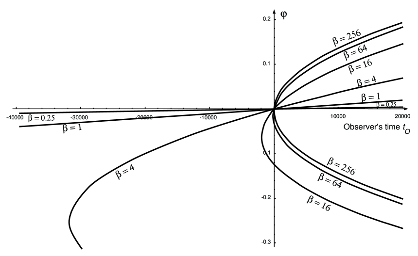
Figure 5: The apparent angular positions of an object traveling at different speeds at a distance $y$ of one million light years from us. The angular positions ($\varphi$ in radians) are plotted against the observer’s time ${t_{\textit{O}}}$ in years.

This discussion shows that a single object moving across our field of vision at superluminal speed creates an illusion of an object appearing at a certain point in time, stretching and splitting into two and then moving away from each other. This time evolution of the two objects is given in Eq. (1), and illustrated in the bottom panel of Fig. 4(b). Note that the apparent time ${t_{\textit{O}}}$ (as perceived by the observer) is reversed with respect to the real time $t$ in the region $A_{-}$ to $B^{\prime}$. An event that happens near $B^{\prime}$ appears to happen before an event near $A_{-}$. Thus, the observer may see an apparent violation of causality, but it is only a part of the light travel time effect.

If there are multiple objects, moving as a group, at roughly constant superluminal speed along the same direction, they will appear as a series of objects materializing at the same angular position and moving away from each other sequentially, one after another. The apparent knot in one of the jets always has a corresponding knot in the other jet. In fact, the appearance of a superluminal knot in one of the jets with no counterpart in the opposite jet, or a clear movement in the angular position of the “core” (at point $B^{\prime}$) will invalidate our model.

3 Redshifts of the Hotspots

In the previous section, we showed how a hypothetical superluminal object appears as two objects receding from a core. Now we consider the time evolution of the redshift of the two apparent objects (or hotspots). Since the relativistic Doppler shift equation is not appropriate for our considerations (because we are working with hypothetical superluminal objects), we need to work out the relationship between the redshift (z) and the speed ($\beta$) as we would do for sound. This calculation is done in Appendix A.1:

$$1\,+\,{\text{z}}\, = \,\left|1\,-\,\beta\cos\theta\right|$$

$$= \,\left|1\,+\,\beta\sin\varphi\right|$$

$$= \,\left|1\,+\,\frac{\beta^{2}t}{\sqrt{\beta^{2}t^{2}+y^{2}}}\right|$$ (3)

We can explain the radio frequency spectra of the hotspots as extremely redshifted black body radiation because $\beta$ can be enormous in our model of extragalactic radio sources. Note that the limiting value of $|1+{\text{z}}|$ is approximately equal to $\beta$, which gives an indication of the speeds required to push the black body radiation of a typical star to the RF region. Since the speeds ($\beta$) involved are typically extremely large, and we can approximate the redshift as:

$$1\,+\,{\text{z}}\,\approx\,\left|\beta\varphi\right|\,\approx\,\frac{\left|\beta\Phi\right|}{2}$$

Assuming the object to be a black body similar to the sun, we can predict the peak wavelength (defined as the wavelength at which the luminosity is a maximum) of the hotspots as:

$$\lambda_{\text{max}}\,\approx\,(1+{\text{z}})480nm\,\approx\,\frac{\left|\beta\Phi\right|}{2}480nm$$

where $\Phi$ is the angular separation between the two hotspots.

This equation shows that the peak RF wavelength increases linearly with the angular separation. If multiple hotspots can be located in a twin jet system, their peak wavelengths will depend only on their angular separation, in a linear fashion. Such a measurement of the emission frequency as $\varphi$ increases along the jet is clearly seen in the photometry of the jet in 3C 273.[10] Furthermore, if the measurement is done at a single wavelength, intensity variation can be expected as the hotspot moves along the jet. In other words, measurements at higher wavelengths will find the peak intensities farther away from the core region, which is again consistent with observations.

4 Gamma Ray Bursts

The evolution of redshift of the thermal spectrum of a hypothetical superluminal object also holds the explanation for gamma ray bursts (GRBs).

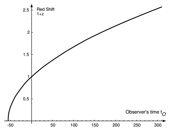
Figure 6: Time evolution of the redshift from a superluminal object. It shows the redshifts expected from an object moving at $\beta=300$ at a distance of ten million light years from us. The X axis is the observer’s time in years. (Since the X axis scales with time, it is also the redshift from an object at 116 light days –ten million light seconds– with the X axis representing ${t_{\textit{O}}}$ in seconds.)

The evolution of GRB can be made quantitative because we know the dependence of the observer’s time ${t_{\textit{O}}}$ and the redshift $1+{\text{z}}$ on the real time $t$ (Eqs. (1) and (3)). From these two, we can deduce the observed time evolution of the redshift (see Appendix A.3). We have plotted it parametrically in Fig. 6 that shows the variation of redshift as a function of the observer’s time (${t_{\textit{O}}}$). The figure shows that the observed spectra of a superluminal object is expected to start at the observer’s time ${t_{\textit{O}}}_{\text{min}}$ with heavy (infinite) blue shift. The spectrum of the object rapidly softens and soon evolves to zero redshift and on to higher values. The rate of softening depends on the speed of the underlying superluminal object and its distance from us. The speed and the distance are the only two parameters that are different between GRBs and symmetric radio sources in our model.

Note that the X axis in Fig. 6 scales with time. We have plotted the variation of the redshift ($1+{\text{z}}$) of an object with $\beta=300$ and $y=$ ten million light years, with X axis is ${t_{\textit{O}}}$ in years. It is also the variation of the redshift of an object at $y=$ ten million light seconds (or 116 light days) with X axis in seconds. The former corresponds to symmetric jets and the latter to a GRB. Thus, for a GRB, the spectral evolution takes place at a much faster pace. Different combinations of $\beta$ and $y$ can be fitted to describe different GRB spectral evolutions.

The observer sees no object before ${t_{\textit{O}}}_{\text{min}}$. In other words, there is a definite point in the observer’s time when the GRB is “born”, with no indication of its impending birth before that time. This birth does not correspond to any cataclysmic event (as would be required in the collapsar/hypernova or the “fireball” model) at the distant object. It is nothing but an artifact of our perception.

In order to compare the time evolution of the GRB spectra to the ones reported in the literature, we need to get an analytical expression for the redshift (z) as a function of the observer’s time (${t_{\textit{O}}}$). This can be done by eliminating $t$ from the equations for ${t_{\textit{O}}}$ and $1+{\text{z}}$ (Eqs. (1) and (3)), with some algebraic manipulations as shown in Appendix A.3. The algebra can be made more manageable by defining $\tau=y/\beta$, a characteristic time scale for the GRB (or the radio source). This is the time the object would take to reach us, if it were coming directly toward us. We also define the age of the GRB (or radio source) as $t_{\text{age}}={t_{\textit{O}}}-{t_{\textit{O}}}_{\text{min}}$. This is simply the observer’s time (${t_{\textit{O}}}$) shifted by the time at which the object first appears to him (${t_{\textit{O}}}_{\text{min}}$). With these notations (and for small values $t$), it is possible to write the time dependence of z as:

$$1+{\text{z}}=\left|{1+\frac{{\beta^{2}\left({-\tau\pm\sqrt{2\beta t_{\text{age}}}}\right)}}{{\beta t_{\text{age}}+\tau/2\mp\sqrt{2\beta t_{\text{age}}}+\beta^{2}\tau}}}\right|$$ (4)

for small values of $t\ll\tau$.

Since the peak energy of the spectrum is inversely proportional to the redshift, it can be written as:

$$E_{\text{pk}}(t_{\text{age}})=\frac{E_{\text{pk}}({t_{\textit{O}}}_{\text{min}})}{1+C_{1}\,\sqrt{\frac{t_{\text{age}}}{\tau}}+C_{2}\,\frac{t_{\text{age}}}{\tau}}$$ (5)

where $C_{1}$ and $C_{2}$ are coefficients to be estimated by the Taylor series expansion of Eq. (4) or by fitting.

Ref. GRB6 have studied the evolution of the peak energy ($E_{\text{pk}}(t)$), and modeled it empirically as:

$$E_{\text{pk}}(t)=\frac{E_{\text{pk,0}}}{(1+t/\tau)^{\delta}}$$ (6)

where $t$ is the time elapsed after the onset ($=t_{\text{age}}$ in our notation), $\tau$ is a time constant and $\delta$ is the hardness intensity correlation (HIC). Ref. GRB6 reported seven fitted values of $\delta$. We calculate their average as $\delta=1.038\pm 0.014$, with the individual values ranging from $0.4$ to $1.1$. Although it may not rule out or validate either model within the statistics, the $\delta$ reported may fit better to Eq. (5). Furthermore, it is not an easy fit because there are too many unknowns. However, the similarity between the shapes of Eqs. (5) and (6) is remarkable, and points to the agreement between our model and the existing data.

5 Conclusions

In this article, we looked at the spatio-temporal evolution of a supersonic object (both in its position and the sound frequency we hear). We showed that it closely resembles GRBs and DRAGNs if we were to extend the calculations to light, although a luminal boom would necessitate superluminal motion and is therefore forbidden.

This difficulty notwithstanding, we presented a unified model for Gamma Ray Bursts and jet like radio sources based on bulk superluminal motion. We showed that a single superluminal object flying across our field of vision would appear to us as the symmetric separation of two objects from a fixed core. Using this fact as the model for symmetric jets and GRBs, we explained their kinematic features quantitatively. In particular, we showed that the angle of separation of the hotspots was parabolic in time, and the redshifts of the two hotspots were almost identical to each other. Even the fact that the spectra of the hotspots are in the radio frequency region is explained by assuming hyperluminal motion and the consequent redshift of the black body radiation of a typical star. The time evolution of the black body radiation of a superluminal object is completely consistent with the softening of the spectra observed in GRBs and radio sources. In addition, our model explains why there is significant blue shift at the core regions of radio sources, why radio sources seem to be associated with optical galaxies and why GRBs appear at random points with no advance indication of their impending appearance.

Although it does not address the energetics issues (the origin of superluminality), our model presents an intriguing option based on how we would perceive hypothetical superluminal motion. We presented a set of predictions and compared them to existing data from DRAGNs and GRBs. The features such as the blueness of the core, symmetry of the lobes, the transient $\gamma$ and X-Ray bursts, the measured evolution of the spectra along the jet all find natural and simple explanations in this model as perceptual effects. Encouraged by this initial success, we may accept our model based on luminal boom as a working model for these astrophysical phenomena.

It has to be emphasized that perceptual effects can masquerade as apparent violations of traditional physics. An example of such an effect is the apparent superluminal motion,[12, 13, 14] which was explained and anticipated within the context of the special theory of relativity[15] even before it was actually observed.[16] Although the observation of superluminal motion was the starting point behind the work presented in this article, it is by no means an indication of the validity of our model. The similarity between a sonic boom and a hypothetical luminal boom in spatio-temporal and spectral evolution is presented here as a curious, albeit probably unsound, foundation for our model.

One can, however, argue that the special theory of relativity (SR) does not deal with superluminality and, therefore, superluminal motion and luminal booms are not inconsistent with SR. As evidenced by the opening statements of Einstein s original paper,[15] the primary motivation for SR is a covariant formulation of Maxwell s equations, which requires a coordinate transformation derived based partly on light travel time (LTT) effects, and partly on the assumption that light travels at the same speed with respect to all inertial frames. Despite this dependence on LTT, the LTT effects are currently assumed to apply on a space-time that obeys SR. SR is a redefinition of space and time (or, more generally, reality) in order to accommodate its two basic postulates. It may be that there is a deeper structure to space-time, of which SR is only our perception, filtered through the LTT effects. By treating them as an optical illusion to be applied on a space-time that obeys SR, we may be double counting them. We may avoid the double counting by disentangling the covariance of Maxwell s equations from the coordinate transformations part of SR. Treating the LTT effects separately (without attributing their consequences to the basic nature of space and time), we can accommodate superluminality and obtain elegant explanations of the astrophysical phenomena described in this article. Our unified explanation for GRBs and symmetric radio sources, therefore, has implications as far reaching as our basic understanding of the nature of space and time.

Appendix A Mathematical Details

A.1 Doppler Shift

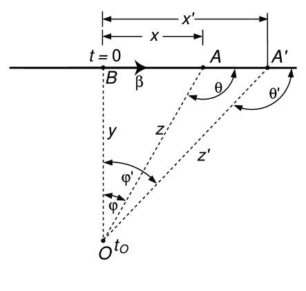
Figure 7: The object is flying along $BAA^{\prime}$, the observer is at $O$. The object crosses $B$ (the point of closest approach) at time $t=0$. It reaches $A$ at time $t$. A photon emitted at $A$ reaches $O$ at time ${t_{\textit{O}}}$, and a photon emitted at $A^{\prime}$ reaches $O$ at time ${t_{\textit{O}}}^{\prime}$.

We refer to Fig. 7 and start by defining the real speed of the object as:

$$v\,=\,\beta\,c\,=\,\frac{x^{\prime}\,-\,x}{t^{\prime}-t}$$ (7)

But the speed it appears to have will depend on when the observer senses the object at $A$ and $A^{\prime}$. The apparent speed of the object is:

$$v^{\prime}\,=\,{\beta_{\textit{O}}}\,c\,=\,\frac{x^{\prime}\,-\,x}{{t_{\textit{O}}}^{\prime}\,-\,{t_{\textit{O}}}}$$ (8)

We also have

$${t_{\textit{O}}}\, = \,t+\frac{z}{c}$$

$${t_{\textit{O}}}^{\prime}\, = \,t^{\prime}+\frac{z^{\prime}}{c}$$

$$\Rightarrow{t_{\textit{O}}}^{\prime}-{t_{\textit{O}}}\, = \,t^{\prime}-t+\frac{z^{\prime}-z}{c}$$ (9)

Thus,

$$\frac{\beta}{{\beta_{\textit{O}}}}\, = \,\frac{{t_{\textit{O}}}^{\prime}-{t_{\textit{O}}}}{t^{\prime}-t}$$

$$= \,1+\frac{z^{\prime}-z}{c(t^{\prime}-t)}$$

$$= \,1-\frac{x-x^{\prime}}{c(t^{\prime}-t)}\cos\theta$$

$$= \,1-\beta\cos\theta$$ (10)

which gives,

$${\beta_{\textit{O}}} \,=\, \frac{\beta}{1\,-\,\beta\cos\theta}$$

$$\beta \,=\, \frac{{\beta_{\textit{O}}}}{1\,+\,{\beta_{\textit{O}}}\cos\theta}$$ (11)

and,

$$\frac{{\beta_{\textit{O}}}}{\beta} \,=\, \frac{1}{1-\beta\,\cos\theta}$$ (12)

$$\,=\, 1+{\beta_{\textit{O}}}\,\cos\theta$$

$$\,=\, \sqrt{\frac{1+{\beta_{\textit{O}}}\,\cos\theta}{1-\beta\,\cos\theta}}$$

Redshift (z) defined as:

$$1\,+\,{\text{z}}\,=\,\frac{{\lambda_{\textit{O}}}}{\lambda}$$ (13)

where ${\lambda_{\textit{O}}}$ is the measured wavelength and $\lambda$ is the known wavelength. In Fig. 7, the number of wave cycles created in time $t^{\prime}-t$ between $A$ and $A^{\prime}$ is the same as the number of wave cycles sensed at $O$ between ${t_{\textit{O}}}^{\prime}$ and ${t_{\textit{O}}}$. Substituting the values, we get:

$$\frac{(t^{\prime}-t)\,c}{\lambda}\,=\,{\frac{({t_{\textit{O}}}^{\prime}\,-\,{t_{\textit{O}}})\,c}{{\lambda_{\textit{O}}}}}$$ (14)

Using the definitions of the real and apparent speeds from Eqs. (7) and (8), it is easy to get:

$$\frac{{\lambda_{\textit{O}}}}{\lambda}\,=\,\frac{\beta}{{\beta_{\textit{O}}}}$$ (15)

Using the relationship between the real speed $\beta$ and the apparent speed ${\beta_{\textit{O}}}$ from Eq. (12), we get:

$$1\,+\,{\text{z}}\, = \,\frac{1}{1\,+\,{\beta_{\textit{O}}}\cos\theta}$$

$$= \,1\,-\,\beta\cos\theta$$ (16)

As expected, z depends on the longitudinal component of the velocity of the object. Since we allow superluminal speeds in this calculation, we need to generalize this equation for z noting that the ratio of wavelengths is positive. Taking this into account, we get:

$$1\,+\,{\text{z}}\, = \,\left|\frac{1}{1\,+\,{\beta_{\textit{O}}}\cos\theta}\right|$$

$$= \,\left|1\,-\,\beta\cos\theta\right|$$ (17)

For a receding object $\theta=\pi$. If we consider only subluminal speeds, we can rewrite this as:

$$1\,+\,{\text{z}}\, = \,\frac{1}{1\,-\,{\beta_{\textit{O}}}}$$

$$= \,1\,+\,\beta$$

$$(1\,+\,{\text{z}})^{2}\, = \,\frac{1\,+\,\beta}{1\,-\,{\beta_{\textit{O}}}}$$

Or,

$$1\,+\,{\text{z}}\,=\,\sqrt{\frac{1+\beta}{1\,-\,{\beta_{\textit{O}}}}}$$ (18)

If we were to mistakenly assume that the speed we observe is the real speed, then this becomes the relativistic Doppler formula:

$$1\,+\,{\text{z}}\,=\,\sqrt{\frac{1+\beta}{1\,-\,\beta}}$$ (19)

A.2 Kinematics of Superluminal Objects

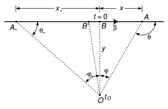
Figure 8: An object flying along $A_{-}BA$ at a constant superluminal speed. The observer is at $O$. The object crosses $B$ (the point of closest approach to $O$) at time $t=0$.

The derivation of the kinematics is based on Fig. 8. Here, an object is moving at a superluminal speed along $A_{-}BA$. At the point of closest approach, $B$, the object is a distance of $y$ from the observer at $O$. Since the speed is superluminal, the light emitted by the object at some point $B^{\prime}$ (before the point of closest approach $B$) reaches the observer before the light emitted at $A_{-}$. This gives an illusion of the object moving in the direction from $B^{\prime}$ to $A_{-}$, while in reality it is moving from $A_{-}$ to $B^{\prime}$.

Observed angle $\varphi$ is measured with respect to the point of closest approach $B$ and is defined as $\theta-\pi/2$ where $\theta$ is the angle between the object’s velocity and the observer’s line of sight. $\varphi$ is negative for negative time $t$. We choose units such that $c=1$ for simplicity and denote the observer’s time by ${t_{\textit{O}}}$. Note that, by definition, the origin in the observer’s time, ${t_{\textit{O}}}$ is set to the instant when the object appears at $B$.

The real position of the object at any time $t$ is:

$$x=y\tan\varphi=\beta t$$ (20)

Or,

$$t=\frac{y\tan\varphi}{\beta}$$ (21)

A photon emitted by the object at $A$ (at time $t$) will reach $O$ after traversing the hypotenuse. A photon emitted at $B$ will reach the observer at $t=y$, since we have chosen $c=1$. Since we define the observer’s time ${t_{\textit{O}}}$ such that the time of arrival is $t={t_{\textit{O}}}+y$, then we have:

$${t_{\textit{O}}}=t+\frac{y}{\cos\varphi}-y$$ (22)

which gives the relation between ${t_{\textit{O}}}$ and $\varphi$.

$${t_{\textit{O}}}=y\left(\frac{\tan\varphi}{\beta}+\frac{1}{\cos\varphi}-1\right)$$ (23)

Expanding the equation for ${t_{\textit{O}}}$ to second order, we get:

$${t_{\textit{O}}}=y\left(\frac{\varphi}{\beta}+\frac{\varphi^{2}}{2}\right)$$ (24)

The minimum value of ${t_{\textit{O}}}$ occurs at $\varphi_{0}=-1/\beta$ and it is ${t_{\textit{O}}}_{\text{min}}=-y/2\beta^{2}$. To the observer, the object first appears at the position $\varphi=-1/\beta$. Then it appears to stretch and split, rapidly at first, and slowing down later.

The quadratic Eq. (24) can be recast as:

$$1+\frac{2\beta^{2}}{y}{t_{\textit{O}}}=\left(1+\beta\varphi\right)^{2}$$ (25)

which will be more useful later in the derivation.

The angular separation between the objects flying away from each other is the difference between the roots of the quadratic Eq. (24):

$$\Phi\, = \,\varphi_{1}-\varphi_{2}$$

$$= \,\frac{2}{\beta}\sqrt{1+\frac{2\beta^{2}}{y}{t_{\textit{O}}}}$$

$$= \,\frac{2}{\beta}\left(1+\beta\varphi\right)$$ (26)

making use of Eq. (25). Thus, we have the angular separation either in terms of the observer’s time ($\Phi({t_{\textit{O}}})$) or the angular position of the object ($\Phi(\varphi)$) as illustrated in Figure 9.

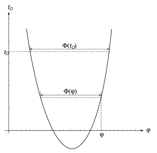
Figure 9: Illustration of how the angular separation is expressed either in terms of the observer’s time ($\Phi({t_{\textit{O}}})$) or the angular position of the object ($\Phi(\varphi)$)

The rate at which the angular separation occurs is:

$$\frac{d\Phi}{d{t_{\textit{O}}}}\, = \,\frac{2\beta}{y\sqrt{1+\frac{2\beta^{2}}{y}{t_{\textit{O}}}}}$$

$$= \,\frac{2\beta}{y\left(1+\beta\varphi\right)}$$ (27)

Again, making use of Eq. (25). Defining the apparent age of the radio source $t_{\text{age}}={t_{\textit{O}}}-{t_{\textit{O}}}_{\text{min}}$ and knowing ${t_{\textit{O}}}_{\text{min}}=-y/2\beta^{2}$, we can write:

$$\frac{d\Phi}{d{t_{\textit{O}}}}\, = \,\frac{2\beta}{y\sqrt{1+\frac{2\beta^{2}}{y}{t_{\textit{O}}}}}$$

$$= \,\frac{2\beta}{y\sqrt{1-\frac{{t_{\textit{O}}}}{{t_{\textit{O}}}_{\text{min}}}}}$$

$$= \,\sqrt{\frac{4\beta^{2}}{y^{2}}\,\times\,\frac{-{t_{\textit{O}}}_{\text{min}}}{{t_{\textit{O}}}-{t_{\textit{O}}}_{\text{min}}}}$$

$$= \,\sqrt{\frac{2}{y\,t_{\text{age}}}}$$ (28)

A.3 Time Evolution of the Redshift

As shown before in Eq. (17), the redshift z depends on the real speed $\beta$ as:

$$1\,+\,{\text{z}}\,=\,\left|1\,-\,\beta\cos\theta\right|\,=\,\left|1\,+\,\beta\sin\varphi\right|$$ (29)

For any given time (${t_{\textit{O}}}$) for the observer, there are two solutions for $\varphi$ and z. $\varphi_{1}$ and $\varphi_{2}$ lie on either side of $\varphi_{0}=1/\beta$. For $\sin\varphi>-1/\beta$, we get

$$1+{\text{z}}_{2}=1+\beta\sin\varphi_{1}$$ (30)

and for $\sin\varphi<-1/\beta$,

$$1+{\text{z}}_{1}=-1-\beta\sin\varphi_{2}$$ (31)

Thus, we get the difference in the redshift between the two hotspots at $\varphi_{1}$ and $\varphi_{2}$ as:

$$\Delta{\text{z}}\approx 2+\beta(\varphi_{1}+\varphi_{2})$$ (32)

We also have the mean of the solutions of the quadratic ($\varphi_{1}$ and $\varphi_{2}$) equal to the position of the minimum ($\varphi_{0}$):

$$\frac{\varphi_{1}+\varphi_{2}}{2}=-\frac{1}{\beta}$$ (33)

Thus $\varphi_{1}+\varphi_{2}=-2/\beta$ and hence $\Delta{\text{z}}=0$. The two hotspots will have identical redshifts, if terms of $\varphi^{3}$ and above are ignored.

As shown before (see Eq. (29)), the redshift z depends on the real speed $\beta$ as:

$$1\,+\,{\text{z}}\,=\,\left|1\,+\,\beta\sin\varphi\right|\,=\,\left|1\,+\,\frac{\beta^{2}t}{\sqrt{\beta^{2}t^{2}+y^{2}}}\right|$$ (34)

Since we know z and ${t_{\textit{O}}}$ functions of $t$, we can plot their inter-dependence parametrically. This is shown in Fig. 6 of the article.

It is also possible to eliminate $t$ and derive the dependence of $1+{\text{z}}$ on the apparent age of the object under consideration, $t_{\text{age}}={t_{\textit{O}}}-t_{\text{min}}$. In order to do this, we first define a time constant $\tau=y/\beta$. This is the time the object would take to reach us, if it were flying directly toward us. Keeping in mind that the new variable is related to $t_{\text{age}}$ through ${t_{\textit{O}}}_{\text{min}}=-y/2\beta^{2}=-\tau/\beta$, let’s get an expression for $t/\tau$:

$${t_{\textit{O}}}\, = \,t+\sqrt{\beta^{2}t^{2}+y^{2}}-y$$

$$= \,t+\beta\tau\sqrt{1+\frac{{t^{2}}}{{\tau^{2}}}}-\beta\tau$$

$$\approx \,t+\frac{{\beta t^{2}}}{{2\tau}}$$

$$\Rightarrow\frac{t}{\tau}\, = \,\frac{{-1\pm\sqrt{1+\frac{{2\beta t_{\text{age}}}}{\tau}}}}{\beta}$$ (35)

Note that this is valid only for $t\ll\tau$. Now we collect the terms in $t/\tau$ in the equation for $1+{\text{z}}$:

$${t_{\textit{O}}}\, = \,t+\sqrt{\beta^{2}t^{2}+y^{2}}-y$$

$$\Rightarrow\sqrt{\beta^{2}t^{2}+y^{2}}\, = \,{t_{\textit{O}}}-t+y$$

$$1+z\, = \,\left|{1+\frac{{\beta^{2}t}}{{\sqrt{\beta^{2}t^{2}+y^{2}}}}}\right|$$

$$= \,\left|{1+\frac{{\beta^{2}t}}{{{t_{\textit{O}}}-t+y}}}\right|$$

$$= \,\left|{1+\frac{{\beta^{2}\frac{t}{\tau}}}{{\frac{{t_{\text{age}}}}{\tau}-\frac{1}{{2\beta}}-\frac{t}{\tau}+\beta}}}\right|$$ (36)

As expected, the time variables always appear as ratios like $t/\tau$, giving confidence that our choice of the characteristic time scale is probably right. Finally, we can substitute $t/\tau$ from Eq. (35) in Eq. (36) to obtain:

$$1+{\text{z}}=\left|{1+\frac{{\beta^{2}\left({-\tau\pm\sqrt{2\beta t_{\text{age}}}}\right)}}{{\beta t_{\text{age}}+\tau/2\mp\sqrt{2\beta t_{\text{age}}}+\beta^{2}\tau}}}\right|$$ (37)

References

- [1] T. Piran. Int. J. Mod. Phys. A, 17, 2727–2731 (2002).
- [2] E. P. Mazets, S. V. Golenetskii, V. N. Ilyinskii, Yu. A. Guryan, and R. L. Aptekar. Astrophys. Space Sci., 82, 261–282 (1982).
- [3] T. Piran. Phys. Rept., 314, 575–667 (1999).
- [4] F. Ryde. Astrophys. J., 614, 827–846 (2005).
- [5] F. Ryde, , and R. Svensson. Astrophys. J., 566, 210–228 (2003).
- [6] R. A. Perley, J. W. Dreher, and J. J. Cowan. Astrophys. J., 285, L35–L38 (1984).
- [7] I. Owsianik and J. E. Conway. Astron. Astrophys., 337, 69–79 (1998).
- [8] A. G Polatidis, J. E. Conway, and I. Owsianik. In Ros, Porcas, Lobanov, Zensus, editor, Proc. 6th European VLBI Network Symposium (2002).
- [9] G. Ghisellini. Int J. Mod. Phys. A (Proc. 19th European Cosmic Ray Symposium - ECRS 2004) (2004).
- [10] S. Jester, H. J. Roeser, K. Meisenheimer, and R. Perley. Astron. Astrophys., 431, 477–502, (2005).
- [11] F. Ryde and R. Svensson. Astrophys. J., 529, L13–L16 (2000).
- [12] I. F. Mirabel and L. F. Rodríguez. Nature, 371, 46–48, (1994).
- [13] G. Gisler. Nature, 371, 18, (1994).
- [14] J. A. Biretta, W. B. Sparks, and F. Macchetto. Astrophys. J., 520, 621–626, (1999).
- [15] A. Einstein. Ann. der Physik, 17, 891–921 (1905).
- [16] M. Rees. Nature, 211, 468–470 (1966).