Determination of the Physical Conditions of the Knots in the Helix Nebula from Optical and Infrared Observations

Abstract

We use new Hubble Space Telescope and archived images to clarify the nature of the ubiquitous knots in the Helix Nebula, which are variously estimated to contain a significant to majority fraction of the material ejected by its central star.

We employ published far infrared spectrophotometry and existing 2.12 $\mu$m images to establish that the population distribution of the lowest ro-vibrational states of H₂  is close to the distribution of a gas in local thermodynamic equilibrium (LTE) at $988\pm 119$ K. In addition, we present calculations that show that the weakness of the H₂ 0-0 S(7) line is not a reason for making the unlikely-to-be true assumption that H₂ emission is caused by shock excitation.

We derive a total flux from the nebula in H₂ lines and compare this with the power available from the central star for producing this radiation. We establish that neither soft X-rays nor 912–1100 Å radiation has enough energy to power the H₂ radiation, only the stellar extreme ultraviolet radiation shortward of 912 Å does. Advection of material from the cold regions of the knots produces an extensive zone where both atomic and molecular hydrogen are found, allowing the H₂ to directly be heated by Lyman continuum radiation, thus providing a mechanism that will probably explain the excitation temperature and surface brightness of the 2.12 $\mu$m  cusps and tails.

New images of the knot 378-801 in the H₂ 2.12 $\mu$m line reveal that the 2.12 $\mu$m cusp lies immediately inside the ionized atomic gas zone. This property is shared by material in the “tail’ region. The H₂ 2.12 $\mu$m emission of the cusp confirms previous assumptions, while the tail’s property firmly establishes that the “tail” structure is an ionization bounded radiation shadow behind the optically thick core of the knot. The new 2.12 $\mu$m image together with archived Hubble images is used to establish a pattern of decreasing surface brightness and increasing size of the knots with increasing stellar distance. Although the contrast against the background is greater in 2.12 $\mu$m  than in the optical lines, the higher resolution and signal of optical images remains the most powerful technique for searching for knots.

A unique new image of a transitional region of the nebula’s inner disk in the HeII 4686 Å  line fails to show any emission from knots that might have been found in the He⁺⁺ core of the nebula. We also re-examined high signal-to-noise ratio ground-based telescope images of this same inner region and found no evidence of structures that could be related to knots.

1. INTRODUCTION

The dense knots that populate the closest bright planetary nebula NGC 7293 (the Helix Nebula) must play an important role in mass loss from highly evolved intermediate mass stars and therefore in the nature of enrichment of the interstellar medium (ISM) by these stars. It is likely that similar dense condensations are ubiquitous among the planetary nebulae (O’Dell et al. 2002) as the closest five planetary nebulae show similar or related structures. They are an important component of the mass lost by their host stars, for the characteristic mass of individual knots has been reported as $\geq 10^{-5}~{}M_{\odot}$ (from CO emission, Huggins et al. 2002), $5.6\times 10^{-5}~{}M_{\odot}$ (from the dust optical depth determination by Meaburn et al. (1992), adjusted for the improved distance), and about $3.8\times 10^{-5}$ M_⊙ (O’Dell & Burkert 1997, again from the dust optical depth but with better spatial resolution), and their number has been variously estimated to be from 3500 (O’Dell & Handron 1996) from optical observations to much larger numbers (23,000 Meixner et al. 2005, henceforth MX05; 20,000–40,000 Hora et al. 2006, henceforth H06) from infrared imaging. Therefore, these condensations contain a significant fraction to a majority of all the material ejected. It is an extremely important point to understand if the ISM is being seeded by these knots and if they survive long enough to be important in the general properties of the ISM and also the process of formation of new stars. To understand those late phases, long after the knots have escaped the ionizing environment of their central stars, one must understand their characteristics soon after their formation-which is the subject of this study.

There has been a burst of interest in the Helix Nebula and its knots beginning with the lower resolution groundbased study of Meaburn et al. (1992) and the Hubble Space Telescope (HST) images at better than 0.1″ resolution (O’Dell & Handron 1996, O’Dell & Burkert 1997) in the optical window. The entire nebula has been imaged in the H₂ v=1-0 S(1) 2.12 $\mu$m line at scales and resolutions of about 4″ (Speck et al. 2002), and 1.7″/pixel (H06), while Huggins et al. 2002) have studied one small region at 1.2″ resolution, and the NIC3 detector of the NICMOS instrument of the HST has been used by Meixner et al. (2004, MX05) to sample several outer regions at about 0.2″ resolution. A lower resolution ( 2″) study in the longer wavelength 0-0 rovibrational lines has imaged the entire nebula with the Spitzer Space Telescope (H06), extending a similar investigation by Cox et al. (1998, henceforth Cox98) at 6″/pixel with the Infrared Space Observatory. Radio observations of the CO (Huggins et al. 2002, Young et al. 1999) and H I (Rodríguez et al. 2002) emission have even lower spatial resolution, but, the high spectral resolution allows one to see emission from individual knots.

The three dimensional model for the Helix Nebula has also evolved during this time. We now know that the inner part of the nebula is a thick disk of 500″ diameter seen at an angle of about 23° from the plane of the sky (O’Dell et al. 2004, henceforth OMM04). This disk has a central core of high ionization material traced by He II emission (4686 Å), and a series of progressively lower ionization zones until its ionization front is reached. The more easily visible lower ionization portions of the inner-disk form the inner-ring of the nebula. There are polar plumes of material perpendicular to this inner disk extending out to at least 940″ (OMM04) to both the northwest and southeast. There is an apparent irregular outer-ring which Meaburn et al. (2005, henceforth M05) argue is a thin layer of material on the surface of the perpendicular plumes, whereas OMM04) and O’Dell (2005) argue that this is due to a larger ring lying almost perpendicular to the inner disk.

The nature of the knots has attracted considerable attention. O’Dell & Burkert (1997) determined the properties using HST WFPC2 emission line images in H$\alpha$, [N II], and [O III], while O’Dell et al. (2000, henceforth OHB00) analyzed HST slitless spectra of the bright knot 378-801 in H$\alpha$ and [N II], an investigation extended in a study (O’Dell et al, henceforth OHF05) with better slitless images in the same lines and also the [O I] line at 6300 Å. We will adopt the position based designation system described in O’Dell & Burkert (1997) and the trigonometric parallax distance of 219 pc from Harris et al. (2007). The object 378-801 is the best studied of the knots and the primary target for the program reported upon in this paper. At 219 pc distance from the Sun, the 1.5″ chord of the bright cusp surrounding the neutral central core of 378-801 is $4.9\times 10^{15}$ cm. O’Dell & Burkert (1997) estimate that the peak density in the ionized cusp is about 1200 $\rm cm^{-3}$ and the central density of the core, derived from the optical depth in dust, is $4.8\times 10^{5}$ $\rm cm^{-3}$, a number similar to the H₂ density of $\geq$10⁵ $\rm cm^{-3}$ necessary to produce the thermalized population distribution found for the J states within the $v=0$ levels of the electronic (X $\rm{}^{1}\Sigma^{+}_{g}$) ground state by Cox98. Cox98 determined that two sample regions of knots were close to a population distribution of about 900 K, a similar result is found by an analysis (§ 4.2) of new observations (H06) of different regions of knots.

As was argued in O’Dell & Handron (1996), the knots are neutral condensations ionized on the side facing the central star. López-Martín et al. (2001) have shown that the early apparent discrepancy between the observed and predicted surface brightness of the bright cusps is resolved once one considers the dynamic nature of the flow from the cusp ionization front, which depresses the recombination emission from the ionized gas. The central cores are molecular, being visible in CO (Huggins et al. 2002), and producing the multiple velocity components one sees in the low spatial resolution-high velocity resolution CO studies (Young et al. 1999). The H₂ emission is produced in a thin layer of material immediately behind the ionized cusp (Huggins et al. 2002). OHB00 show that the optical structure within the ionized cusp can only be explained if the material is heated on a timescale that is longer than the time for cool material to flow from the ionization front across the width of the cusp. This slow heating rate means that forbidden lines are seen only further away from the ionization front (because these require energetic electrons to cause their collisional excitation) whereas recombination lines like H$\alpha$ arise preferentially from the cool regions closer to the ionization front. A succession of papers (Burkert & O’Dell 1998; OHB00, OHF05 ) attempting to simultaneously account for both the ionization and flow of material have produced a general model where cool material in the molecular central core flows towards the ionization front, is slowly heated, and upon passing through the ionization front is more rapidly heated and accelerated. At first examination the most recent models look satisfactory. However, the models fail because the theoretically expected zone of 900 K gas has much too low a column density to account for the observed surface brightness in H₂ (OHF05). These H₂ observations must be telling us about something overlooked in previous models. As we discuss in § 4.4, this missing ingredient seems to be that the earlier models were for a static structure, whereas the knots are actually in a state of active flow.

This paper reports on work intended to clarify the nature of the knots in the Helix Nebula. New observations with all three of the imaging instruments on the HST were made and are described in § 2, then analyzed in § 3. A new and more refined theoretical model is presented in § 4, while these and other recent observations and models are discussed in § 5.

2. OBSERVATIONS

In this investigation we draw on both our own new observations made with the HST and published observations made with a variety of telescopes. These observations range from the optical through the infrared.

2.1. New Observations

The new HST observations were made during eight orbits over the period 2006 May 22-24 as program GO 10628 (co-author O’Dell as Principlal Investigator). The Helix Nebula is sufficiently large that we could simultaneously observe it with the three operating imaging instruments, the WFPC2 (Holtzman et al. 1995), the NICMOS (Thompson et al. 1998), and the ACS (Gonzaga, S. et al. 2005). By careful selection of the pointing and orientation of the spacecraft, we were able to sample three regions that are useful for understanding the knots and their structure. In each case the new observations are either unique or of substantially longer exposure time than previous similar observations. The placement of the fields of view are shown in Figure 1.

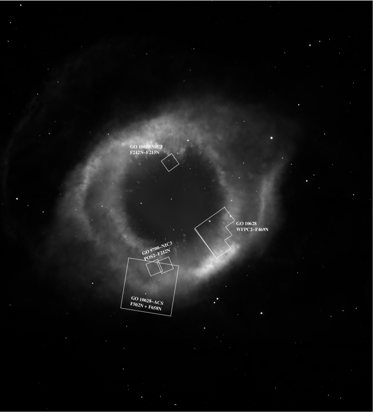
Figure 1.— This 1500″x 1650″ image of the Helix Nebula in H$\alpha$+[N II] from OMM04 shows the fields covered by the three image programs of GO 10628 and also the two NIC3 fields in program GO 9700 that overlap with the GO 10628 ACS field.

2.1.1 NICMOS Images in H₂ of the Knot 378-801

The NICMOS observations were made with the NIC3 camera (256x256 pixels, each about 0.2″/pixel), with eight exposures in both the F212N (isolating the 2.12 $\mu$m H₂ line and the underlying continuum) and the F215N (isolating primarily the underlying continuum as there are no strong lines in this region) filters. Each of the sixteen exposures was 1280 s duration. The pointing was changed in a four position pattern, with steps of 5″. The On-the-Fly standard processing image products were our starting point. These images were combined using IRAF and tasks from the HST data processing STSDAS package provided by the Space Telescope Science Institute (STScI). The method of calibration used in OHF05 was adopted, where the nebular and instrumental continuum was subtracted using the signal from the F215N filter.

The resultant image is shown in Figure 2 along with aligned WFPC2 optical emission line images from programs GO 5086 and 5311. The knot 378-801 is located in the low central region of each image and details of its bright cusp and tail are analyzed in § 3.1 and § 3.2. It is notable that all of the H₂ cusps have corresponding H$\alpha$ and [N II] counterparts and that all of the H$\alpha$ and [N II] cusps have H₂ counterparts on these well exposed, high resolution images.

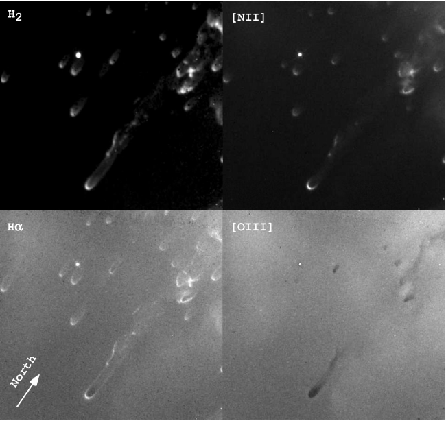
Figure 2.— Each image in this mosaic depicts the same 47.5″x 44.8″region targeted with the NICMOS NIC3 camera. The H₂ image Jis from GO 10628, as described in the text, while the optical emission line images are from WFPC2 programs GO 5086 and 5311. The vertical axis is pointed towards a position angle (PA) of 35°. The NIC3 images have been scaled to the 0.0996″/pixel scale of the WFPC2 camera.

2.1.2 ACS Images of a Southsoutheast Field Previously Observed with NICMOS in H₂

A field to the southsoutheast of the central star and falling into the outer-ring portion of the Helix Nebula was imaged with the ACS camera. Eight exposures of nominally 1200 s each were made in both the F658N filter (which passes the H$\alpha$ and [N II] 6583 Å lines equally well) and the F502N filter (dominated by the [O III] 5007 Å line). The field of view shown in Figure 1 overlaps only slightly with the ACS mosaic built up during the GO 9700 survey with the same filter pairs (OMM04). The signal to noise ratio was much higher than in the GO 9700 survey since that study used total exposures of about 850 s in both of filters.

The images in the four offset pointings were combined using tasks within the STSDAS package. No attempt at absolute calibration was made because of the F658N filter requiring additional observations with the F660N filter, which is dominated by [N II] (O’Dell 2004). The resulting image for F658N is shown in Figure 3. Originally of 0.05″ pixels, it has been averaged into 2x2 samples in order to increase the signal to noise ratio. Since the finest features are larger than the size of the resultant pixels (0.1″) no loss of detail was incurred. The F502N image is much lower signal and is not presented here, although portions of it are reproduced and discussed in § 3.4.

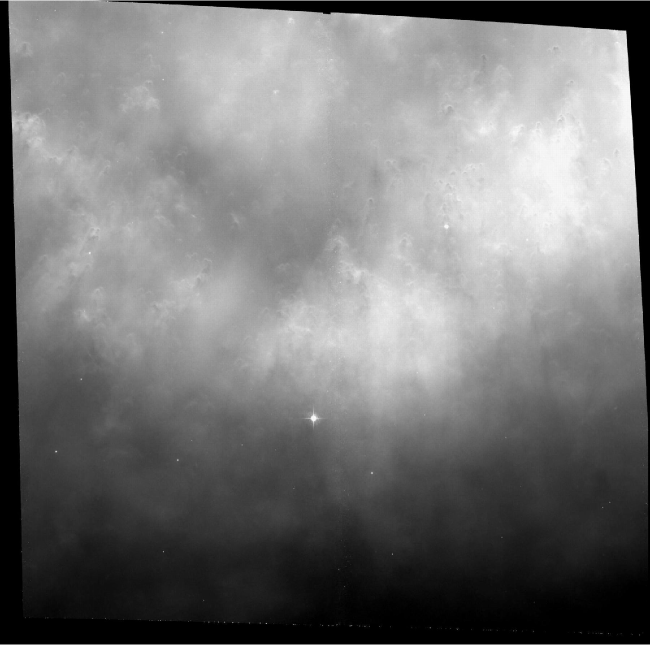
Figure 3.— This high contrast 215″x 213″ image of the ACS region shown in Figure 1 has the vertical axis pointed towards PA=350°. It demonstrates that bright cusp knots are found in the outer-ring of the nebula, in addition to the inner-ring knots that dominate the field covered by the GO 9700 mosaic.

2.1.3 WFPC2 Images in the He II filter of a Southwest Field

Sixteen exposures of 1100 s each were made with the WFPC2 F469N filter that isolates the He II recombination line at 4686 Å. The images from the four pointings were combined using the STSDAS package of dither tasks and the results are shown in Figure 4. For comparison, a matching section of the ACS mosaic that was derived as part of program GO 9700 (OMM04) is also shown.

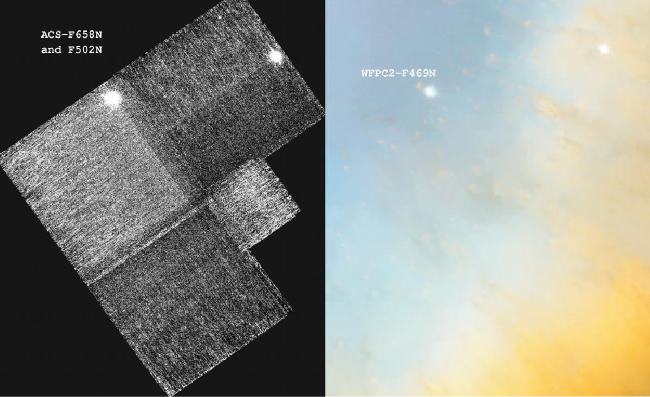
Figure 4.— The left panel shows a 167″x 204″ WFPC2 F469N image with north as the vertical axis and is the result of combining 16 dithered images. For comparison,the right hand panel shows the same section of the nebula from a mosaic of ACS images (OMM04) with H$\alpha$+[N II] as red, an average of H$\alpha$+[N II] and [O III] as green, and [O III] as blue. No indication of features showing HeII 4686Å emission is seen.

2.2. Recently Published Observations

There are three recent papers that contain observations pertinent to our discussion of the nature of the knots in the Helix Nebula. These include two space infrared observations and one groundbased study.

2.2.1 Spitzer Space Telescope Infrared Images and Spectra

In a recent paper H06 present the results of an extensive observational study of the Helix Nebula. They have imaged the object out to the northeast-arc (OMM04) with the IRAC camera (Fazio et al. 2004) in four broad filters centered on 3.6 $\mu$m, 4.5 $\mu$m, 5.8 $\mu$m, and 8.0 $\mu$m. These filters are dominated by emission from rovibrational lines within the $v=0$ ground electronic state, although an atomic continnum must be present in addition to a few collisionally excited forbidden and recombination emission lines. The resolution of these images is about 2″, so that one cannot resolve structure within the cusps, but one can see structure along radial lines passing through the bright cusps and their much longer tails. Spectra were obtained with the IRS (Houck et al. 2004) at three positions, two falling in the outer-ring at locations north and southwest of the central star and the third location (used for background subtraction) falling directly on the fainter northeast-arc feature. They present calibrated fluxes for rovibrational lines of H₂ from 0-0 S(7) at 5.51 $\mu$m out to 0-0 S(1) at 17.0 $\mu$m. They also present a groundbased image in a filter centered on the 2.12 $\mu$m H₂ line which is of comparable spatial resolution but wider field of view that the Speck et al. (2002) study. This image is not flux calibrated but appears to go fainter than the Speck et al. (2002) image.

2.2.2 HST GO 9700 images in H₂

In the program GO 9700 study that produced a continuous mosaic of ACS images MX05 also obtained parallel NIC3 images in the F212N filter at six science positions and one sky position. Each position was actually a double exposure of two pointings, which allowed a slight overlap of the NIC3 fields. The total exposure at each position was about 750 s and double that in the regions of overlap. The method of calibration was different as only F212N images were obtained (the few F175W images were not useful for calibration of the F212N images). It was assumed that the sky images included all the background signal that need to be subtracted, which means that it did not subtract nebular continuum. The NIC3 images are under-sampled (the pixel size of 0.2″ is about the same as the telescope’s resolution at this wavelength) as in our new observations of the field around 378-801. When comparing the data, one should note that the maximum effective exposure time is about 1500 s for the GO 9700 F212N images, while in our study it is 10,240 s. As discussed in § 3.4, our ACS field overlaps with much of the MX05 position 2 field, allowing a more meaningful comparison of optical and infrared images of this region than was possible in the MX05 study.

3. Analysis of the Observations

These new images of the Helix Nebula with three different HST cameras provide new information on a number of subjects related to the nature and formation of the knots. The NICMOS H₂ image allows a discussion of the cusp and tail structure, the He II image places constraints on the location of the knots to the southwest, and the ACS images allow a more complete comparison of early H₂ images to the south and southeast with comparable resolution optical emission line images.

3.1. Stratification in the Bright Cusp of 378-801

The new NIC3 H₂ 2.12 $\mu$m line observations were scaled to the same pixel size as the WFPC2 (0.0996″/pixel) using bilinear interpolation and carefully aligned. Although this region has been imaged numerous times in this line, this is clearly the best image in terms of both its resolution and signal. The three primary optical line images and the new H₂ image are shown in Figure 2. In order to make a quantitative analysis, the images were rotated and a sample three pixels wide along the axis of the cusp-core-tail was made. The results are shown in Figure 5, where the peak value of the H₂ 2.12 $\mu$m and [NII] emission is normalized to unity as are the outer portions of the [OIII] profiles.

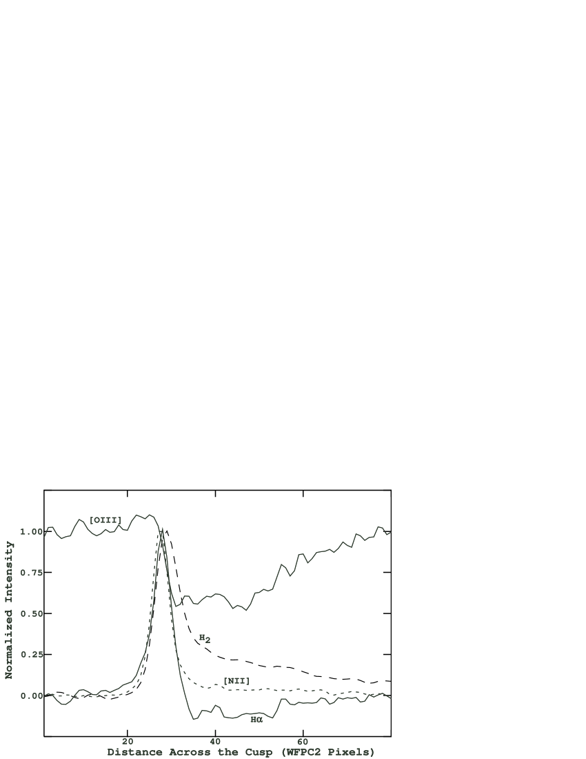
Figure 5.— The normalized intensity of a sample along the axis of knot 378-801 is shown for three optical lines and the H₂ 2.12 $\mu$m infrared line. The 2.12 $\mu$m image has lower resolution (about two pixels) and a comparison of the appearance in the different lines is discussed in the text.

The optical line results are similar to those found by O’Dell & Burkert (1997), Burkert & O’Dell (1998), O’Dell, Henney, & Burkert (2000) and OHF05 in that the ionization occurring furthest from the knots ionization front ([O III]) is weak and extended, this intrinsic low brightness allows one to see the core of the knot in silhouette against the background nebular emission in this line. Although the extinction peaks in the core of the knot, it extends to about 5″ from the bright cusp. The [N II] emission is strong and displaced (0.05″) away from the ionization front with respect to the H$\alpha$ emission. One sees extinction in H$\alpha$ from the core out to almost the same distance as in [O III]. The lack of apparent extinction in [N II] must be due to there being relatively more emission in that line in the sheath of ionized gas surrounding the shadow of the knot. The full width at half maximum (FWHM) of the H$\alpha$ and the [N II] images are 0.48″ and since the FWHM of the stars in the field of view is 0.25″, quadratic subtraction of this instrumental component leaves an intrinsic line width in those emission lines of 0.41″. The FWHM of the H₂ line is 0.61″ and the nearby star’s is 0.42″, leaving an intrinsic FWHM for H₂ of 0.44″ with a peak displaced 0.11″ towards the core of the knot from the H$\alpha$ peak. The FWHM corresponds to a length of $1.40\times 10^{15}$ cm and the displacement to $3.5\times 10^{14}$ cm. The ionized line characteristics are similiar to those found in the previous studies, but we have added here the important characteristic of the small but certain displacement of the broader H₂. The earlier H₂ studies lacked the resolution to determine this characteristic, or in the case of MX05, lacked the high resolution optical lines necessary for the comparison.

The calibrated peak surface brightness in the cusp of 378-801 is $1.8\times 10^{-4}$ $\rm erg~{}cm^{-2}s^{-1}sr^{-1}$ in the H₂ 2.12 $\mu$m line. This agrees well with the peak value of $1.0\times 10^{-4}$ $\rm erg~{}cm^{-2}s^{-1}sr^{-1}$ found by Huggins et al. (2002), where they used the calibration of Speck et al. (2002) and utilized a spatial resolution that would not have recognized the narrowness of the peak.

3.2. Stratification in the Tail of 378-801

The well defined tail in 378-801 is primarily formed by a shadow in the ionizing Lyman Continuum (LyC) radiation cast by the optically thick core, with illumination occurring by diffuse (recombination) LyC photons and direct radiation grazing the edge of the core. The first order theory describing this situation was presented by Cantó et al. (1998) and applied to the tails of the Helix Nebula and the shadows behind the Orion Nebula proplyds soon after (O’Dell 2000). OHF05 discussed the structure in tail of 378-801 within the light of this theory and its next order refinements (Wood et al. 2004), but were unable to explain the details of what was being seen. H₂ in the tails was first detected by Walsh & Ageorges (2003) and we are able to establish with our new observations where this emission arises.

We present in Figure 6 results from traces across the tail of 378-801 extending from 3.1″  to 6.0″ behind the peak of the cusp in H$\alpha$. This region does not extend as far as the partially obscured knot lying on the east side of the tail with its cusp 8.3″ beyond 378-801’s H$\alpha$ cusp. One sees that there is a well defined signature of a limb brightened sheath in both H₂ 2.12 $\mu$m and H$\alpha$, with the peaks of the H₂ emission occuring inside the H$\alpha$, as expected if the H$\alpha$ is associated with a local ionization front. Since the gas ionized by diffuse radiation should be much cooler than the directly illuminated nebular gas, the H$\alpha$ emissivity would be high and the ionized sheath is well defined. These observations establish that conditions in the tail do allow an ionization front to form, while Cantó et al. (1998) and O’Dell (2000) had expected that the shadowed region may be fully ionized. It is not surprising that no [O III] emission is seen, rather, that the dust in the tail, concentrated to the middle of the tail (as noted by OHF05), causes extinction of the background nebular light. The apparent quandary, noted in OHF05, is that the [N II] emission appears to come from inside the ionized sheath of the tail. We already noted that the H$\alpha$ and H₂ structure indicates that an ionization boundary occurs at the edge of the radiation shadow, so there is an apparent contradiction in finding ionized nitrogen emission originating inside an ionization front.

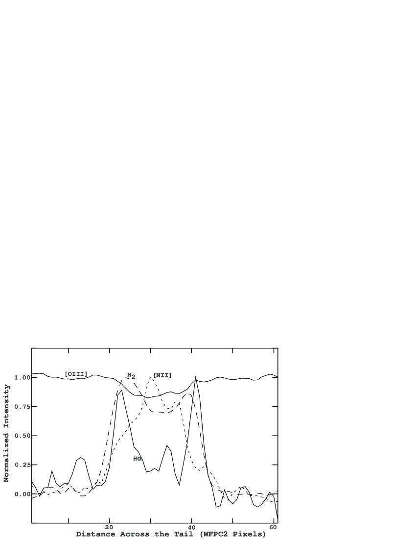
Figure 6.— A cross-section of a tail region of knot 378-901 is shown, with the radiation in each line normalized to unity. The details of the sample and interpretation are presented in the text.

This contradiction is removed by comparison of the [N II] emission and the optical depth, as determined by the [O III] image. Figure 7 shows a comparison of the dust optical depth and the [N II] intensity. The similarity of the distribution of the optical depth and the [N II] brightness argues that the [N II] is actually nebular or cusp light scattered by the only marginally optically thick (peak value $\tau$=0.2 column of dust). This feature is easy to see because the expected low electron temperature of the sheath’s ionization front would suppress the collisionally excited [N II]. If our intepretation of [N II] is correct, then there should be a similar component of scattered H$\alpha$ radiation. This may be what somewhat fills-in the region between the two limb-brightened components (in addition to the low level of surface brightness expected when examining a thin shell). In the cusp [N II] is stronger than H$\alpha$ emission whereas in this part of the nebula the opposite is true. This point argues that much of the scattered [N II] emission arises from the nearby bright cusp, rather than the surrounding nebula.

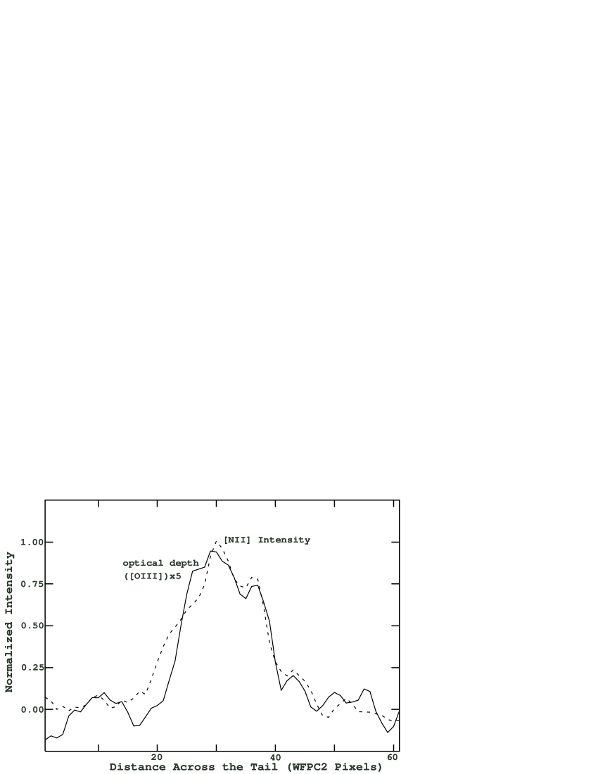
Figure 7.— The normalized surface brightness of the tail sample of Figure 6 is shown together with the optical depth (multiplied by five) determined from the [O III] profile. The similar distribution of each argues that the [N II] emission is caused by scattering of nebular [N II] emission, as discussed in the text.

The distribution along the tail core is discussed in detail in OHF05 (their § 4.1.2) and only a few comments need be added. The question is complex because the knots seem to originate near the nebular ionization front, then are shaped by the radiation field as the ionization front expands beyond them (O’Dell et al. 2002). This means that material in the shadowed region will have never seen direct ionizing radiation and could represent pre-knot material from the planetary nebula’s photon dominated region (PDR). The other source of tail material could be neutral gas accelerated outwards by the rocket effect (e.g. Mellema et al. 1998). Unfortunately, the high velocity resolution study of CO by Huggins et al. (2002) does not really illuminate the question. Their angular resolution was a Gaussian beam of $7.9\arcsec\times 3.8\arcsec$, with the long axis aligned almost along the axis of the tail of 378-801. Since there was a strong CO component coming from the partially shadowed knot lying 8.3″ beyond 378-801’s H$\alpha$ bright cusp, this means that there is a not a clear resolution of the CO emission from the core of 378-801 and the partially shadowed knot. As a result, one cannot hope to interpret the small differences in the position of the peak emission at different velocities as core-tail differences. This could be done with higher spatial resolution CO observations.

3.3. An Unsuccessful Search for He II emission in the Southwest Knots

Figure 4 shows our deep HeII images alongside the same field covered at comparable resolution with the ACS in H$\alpha$+[N II] and [O III]. A detailed comparison of the two images indicates that there is no case of a HeII feature corresponding to a H$\alpha$+[N II] or [O III] feature, nor any HeII only features. The part of the WFPC2 field closest to the central star is 144″ distance. The profile of the HeII core of the central disk, to which the knots in this part of the nebula belong (OMM04) derived from a wide field of view HeII image (O’Dell 1998) shows that the core is down almost to 50% of its peak emission at this distance. If any knots actually occur within the nebula’s HeII core, we would expect that in the simplest knot models, we would see a HeII cusp outside the [O III] zone of each knot and this is not the case. However, the basic model is not that simple.

The detailed models of OHB00 and OHF05 show that the normal progression of ionization states in the cusp are preserved, that is, closest to the ionization front there is an He^o+H⁺ zone, outside of which there is a He⁺+H⁺ zone, and outside of that a He⁺⁺+H⁺. In a nearly constant electron temperature nebula the innermost zone is best traced by the [N II] emission, the next zone by the [O III] emission, and the outermost zone by the HeII emission. Things are not so simple in the case of the knots. As the gas flows through the cusp it is heated only slowly, so that the collisionally excited [N II] emission peaks further out, where the gas is hotter, more than making up for the lower fraction of N⁺ ions. By the time that the second zone is reached the density has dropped significantly and the [O III] emission is broad and weak. One would expect to find a HeII zone associated with a knot only If the knot lies within the nebula’s HeII core. This HeII zone would be quite weak because the density of the knot’s gas would have been greatly decreased this far out. Moreover, the gas has probably nearly reached the temperature of the nebula and these higher temperatures suppress the emission of this recombination line. This means that it will be hard to actually detect by their HeII emission any knots within the HeII core of the nebula. Probably the strongest evidence that no knots exist in the HeII core lies in the fact that we don’t see any objects in extinction in any of the observed emission lines.

3.4. Comparison of the ACS Images in the Southsoutheast with earlier NICMOS H₂ Images

As noted in § 2.1.2, our ACS field overlapped with one of the double-pointings made with NIC3 in F212N as part of program GO 9700 (MX05). MX05 compared their F212N images with the corresponding five fields in OMM04, where the resolution was about 1″and groundbased images were used because the HST ACS mosaic did not extend out this far. This factor of five difference in resolution made it difficult to draw firm conclusions about differences and similarities of appearance. They did, however, conclude that even their short (750 s) overlapping double exposures were sufficient to establish that the knot cusps were more visible in H₂. In § 2.1.1 we showed that in the vicinity of 378-801 that the knots are equally visible in both the ionization cusps and the H₂ cusps.

In Figure 8 we see a comparison of the GO 9700 F212N (H₂) images with our new ACS images. There is an excellent correlation of appearance, although the contrast of the H₂ emission above the essentially zero nebular background is higher than in F658N (H$\alpha$+[N II]) and as usual the knots are only easily seen in the F502N ([O III]) when the knot is in the foreground and can be seen in extinction against the background nebular emission. After considering the flexibility of display of the high signal to noise H$\alpha$+[N II] images, it is difficult to support the conclusion that H₂ 2.12 $\mu$m images are a better way of searching for knot cusps, except for any regions where there is high obscuration.

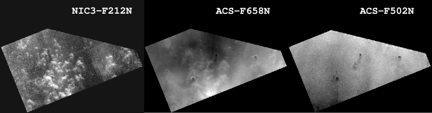
Figure 8.— This figure shows the appearance in the 88″ wide field of overlapping ACS (GO 10628) and NIC3 (GO 9700) images, with north up. The H₂ cusps of the knots are much more visible than the combined H$\alpha$+[N II] ionized cusps. However, close examination shows an ionized gas feature corresponding to each H₂ feature. This is not true for the [O III] F502N features, which require that the knot be located in the foreground. The faint circular features are artifacts of the imaging system.

3.5. Variation in the H₂ Cusps with Distance from the Central Star

Through the new H₂ 2.12 $\mu$m NIC3 images in the current program (GO 10628) and the earlier MX05 study with shorter exposures, there is a larger and hopefully representative sample of resolved H₂ cusps over a wide range of stellar distances ($\phi$). To look for systematic differences, we have identified isolated cusps in each of the fields available. We selected the three closest knots in the GO 10628 field, three in both of MX05’s positions one and two, and two in MX05’s positions three and four, no isolated cusps being available in MX05’s position five. In each case we measured the surface brightness at the peak of the H₂ cusp, the approximate chord across the knot’s center, the width of the H₂ cusp, and determined $\phi$. The GO 10628 and MX05 positions 1-4 had average $\phi$ values of 139″, 290″, 278″, 375″, and 464″ respectively. The average surface brightnesses (in $\rm erg~{}cm^{-2}s^{-1}sr^{-1}$) of the cusp peaks were $1.37\times 10\rm^{-4}$, $7.5\times 10\rm^{-5}$, $8.5\times 10\rm^{-5}$, $4.9\times 10\rm^{-5}$, and $4.5\times 10\rm^{-5}$. The average cusp widths were 0.6″, 0.3″, 0.5″, 0.8″, and 1.1″. The average chord values were 1.5″, 2.5″, 2.2″, 2.4″, and 2.7″.

The most pronounced change in knot characteristic is the cusp peak surface brightness, dropping about linearly with $\phi$, with the cusp width growing slowly and the chord width more steadily with $\phi$. The physical interpretation of these patterns awaits a better understanding of individual knots. It should be pointed out that the relative physical distances from the stars is likely to be increasing more rapidly than the relative values of $\phi$. This is because in the 3-D model of the Helix Nebula in OMM04, the main disk is inclined at an angle about 23° out of the plane of the sky, with the northwest side closer to the observer, while the outer-disk is inclined about 53° out of the plane of the sky, with the southsoutheast side closer to the observer. Objects associated with the inner-disk would have a distance multiplication factor of 1.09 and those in the outer-disk a multiplication factor of 1.66. The objects in the GO 10628 NIC3 field are almost certainly associated with the inner-disk. MX05’s positions 1 and 2 could belong with either system (accurate radial velocities would determine this) and their positions 3 and 4 are almost certainly associated with the outer-disk.

3.6. Comparison of the Structure of the Knots in 2.12 $\mu$m and in H$\alpha$

Figure 2 demonstrates the remarkable similarity of appearance of the knots in H$\alpha$ and in our F212N (2.12 $\mu$m) images and we discussed the quantitative properties of 378-801 in § 3.1 and § 3.2. We have investigated the similarities of the knots by selecting the nine objects (including 378-801) within the NIC3 field of view that are sufficiently isolated to allow a good background subtraction. The peak surface brightness in each cusp was derived in both 2.12 $\mu$m and H$\alpha$ for a sample 3 WFPC2 pixels wide (0.3″). The peak surface brightness in the tail of each object was determined in a sample 11 WFPC2 pixels wide (1.1″) across the tail, the closer end of the sample being 20 WFPC2 pixels (2.0″) displaced from the tip of the bright cusp. We used the 2.12 $\mu$m calibration described in § 2.1.1 and the H$\alpha$ calibration of O’Dell & Doi (1999), expressing the surface brightnesses in units of photons cm^-2 s^-1 sr^-1. The average cusp surface brightness ratio in 2.12 $\mu$m/H$\alpha$ was 5.5$\pm$1.0. The average surface brightness ratio for the tail as compared with the cusp was 0.23$\pm$0.08 in 2.12 $\mu$m and 0.17$\pm$0.05 in H$\alpha$. This means that in the cusp the H₂ 2.12 $\mu$m line alone is putting out more than five times as many photons as in H$\alpha$ and that the contrast between the tail and cusp may be slightly higher (the ratio is lower) in H$\alpha$ than in 2.12 $\mu$m. The remarkable similarity of the knots in a recombination line that follows photoionization of atomic hydrogen and emission in a molecular line heretofore assumed to be the result of radiative pumping between electronic states is discussed in § 4.5.

4. Discussion

Our understanding of the physics of the knots has evolved with a better understanding of a model that satisfactorily explains the knots. The initial descrepancy between the cusp surface brightness and the simplest photoionization model (O’Dell & Handron 1996) was resolved by López-Martín et al. (2001) when it was shown that the advection-dominated nature of the flow through the knot ionization fronts leads to a total rate of recombinations in the ionized gas that is significantly below what is predicted from naive models of ionization equilibrium. The peculiar photoionization structure of H$\alpha$ and [N II] emission can also be understood in similar terms—the heating timescale of the ionized gas is comparable with the dynamic timescales for flow away from the knot surface, leading to resolvable temperature gradients, which strongly affect the relative distribution of recombination line and collisional line emission. The most refined model is that of OHF05, which included both the effects of the radiation field and also the hydrodynamic expansion of the knot’s ionization front. It is probably accurate to say that the photoionized portions of the knots are now adequately understood, or at least that the models are broadly consistent with the best observations.

The structure in the tails is only beginning to be understood. To the first order, the tails are the effects of radiation shadows in the dominant ionizing species, the LyC photons (Cantó et al. 1998, O’Dell 2000). With this paper (§ 3.2) we have now determined that the well observed tails are ionization bounded, with H₂ sheaths inside the zone of ionized gas that occurs at the edge of the LyC shadow. The inner part of the tail is dense enough in dust to scatter surrounding nebular light, although the origin of this material as arising from the original process that forms the knots or as material that is moving back from the knot remains uncertain.

The greatest quandary surrounds the explanation of the H₂ zone that is observed immediately inside the ionized cusps of the knots. The approximate location of this zone of observed H₂ is qualitatively where one would expect it. For reasons given below, it is almost certainly not excited by shocks. Other models (e.g. Natta & Hollenbach 1998) argue that the heating is by absorption of soft X-rays and others that the excitation mechanism is probably fluorescence, where non-ionizing photons from the stellar continuum excite molecules to the B $\rm{}^{1}\Sigma^{+}_{u}$ and C $\rm{}^{1}\Pi_{u}$ electronic states, which then decay, producing the populations of the ground electronic state that give rise to the observed infrared lines. Within the core of the knot the density is sufficiently high and the temperature sufficiently low that multiple heavier molecules are formed and the observed CO is simply the most easily observed abundant tracer of these heavy molecules.

An alternative method of exciting the H₂ molecules is by shocks. At first this idea seems attractive because planetary nebulae as a class are known to possess high velocity stellar winds and large scale mass flows with sufficient energy to excite the low lying energy states of H₂ that give rise to the observed infrared lines. Cox98 first pointed out that the lack of a stellar wind (Cerruti-Sola & Perinotto 1985) rules out excitation by wind-driven shocks. A more complete assessment of shocks as the exciting source was given in OHF05 (their § 4.3.2), where it is shown that although H₂ is heated sufficiently immediately behind a transient shock this shock would quickly move through the knot and up the tail. The well defined location of the H₂ emission zones immediately behind the ionized cusps and the ionized sheath of the tail strongly argues that we are dealing with a quasi-stationary process, rather than something quite dynamic, like shocks.

H06 base their interpretation of H₂ emission on the assumption of shock excitation. Their assumption is based on the weakness of the H₂ 1-1 S(7) line, stating that the radiative models they use predict strong emission in that line, which they do not observe in their spectra. The shortcomings of that criterion for determining that the excitation comes from shocks, rather than radiative processes is discussed below in § 4.1. As we show in § 4.2, the H06 spectra also argue for a high excitation temperature, as found by Cox98. The H06 shock interpretation of the relative population distribution of the H₂ energy states used six free parameters as it required three different shock velocities, each with a different relative intensity. This means that one can’t use the population distribution to confirm that method of excitation.

A key element of understanding the H₂ emission is the excitation temperature of the gas. Cox98 used spectra of the H₂ 0-0 S(2) to S(7) lines to derive the population of their upper states and found that their two sampled regions matched an excitation temperature of 900$\pm$50 K. We show below (§ 4.2) that the new spectra of H06 of the H₂ 0-0 S(1) to S(7) lines in two additional regions agree with the results of Cox98 and support the idea that the H₂ emission comes from gas that is much hotter than the 50 K conditions expected (OHF05) in the core of the knots.

OHF05 demonstrated that even their most detailed PDR models could not explain the high surface brightness in H₂ of the knot cusps, an argument first made by Cox98 from more general considerations. The argument reduces to the fact that the observed surface brightness in H₂ 2.12 $\mu$m radiation is too high to be explained by the column density of 900 K H₂ that is predicted. OHF05 did not have high resolution H₂ 2.12 $\mu$m images of their sample knot (378-801) and a comparison using the results of the new observations reported here are given in § 4.5.

Several papers, including the recent MX05 study, have reported that the surface brightnesses are compatible with earlier the theoretical models of Natta & Hollenbach (1998) in spite of the fact that those authors point out that the knots do not adhere to their general model and would have a higher surface brightness. A more complete critique of earlier claims of agreement of theory and observations is given in OHF05 (§ 4.3.3).

In this section we present the total flux from the central star and nebula in § 4.1, establish that the knots commonly have high excitation temperatures (§ 4.2), show that the absence of strong 1-1 S(7) emission is not a strong argument for shock excitation of the H₂ (§ 4.3), compare the recent data on H₂ emission with the best models (§ 4.4), determine that there is no evidence for radial features extending into the middle of the nebula (§ 4.5), and critique a recent paper that argues for the tails being formed primarily by hydrodynamic processes in § 4.6.

4.1. The Total Flux from the Helix Nebula and its Central Star in Various Energies

The emission from the nebula is in at least quasi-equilibrium with radiation from the central star. This means that the relative fluxes in various nebular and cusp emission lines and in the stellar continuum impose important constraints that must be observed by the correct model for the cusp H₂ emission.

4.1.1 The Central Star

The stellar continuum has been well defined down to 1200 Å by Bohlin et al. (1982), who conclude that the star has a luminosity of $120~{}L_{\odot}$ (corrected to the trigonometric parallax distance) and an effective temperature of 123,000 K. In the long wavelength end of the continuum, the flux per wavelength interval is very close to $\lambda^{-4}$, as expected when one looks at much lower energies than where the peak emission occurs. This total luminosity corresponds to a flux at the Earth of $8.8\times 10^{-8}$ $\rm erg~{}cm^{-2}~{}s^{-1}$.

Natta & Hollenbach (1998) argue that the H₂ is heated by X-rays of greater than 100 eV because only these high energy photons would penetrate the ionization boundary. There are two emitters in the high energy end of the spectrum, the central star and a high temperature component of about (10⁷ K) (Leahy et al. 1994, Leahy et al. 1996, Guerrero et al. 2001). The central star emission in the 0.1-2.0 KeV range is $4\times 10^{-11}$ $\rm erg~{}cm^{-2}~{}s^{-1}$ and the emission from the 10⁷ K component is $9\times 10^{-14}$ (Leahy et al. 1994).

The wavelength range for the fluorescent pumping mechanism is from about 912 Å  to 1100 Å as determined by the minimum energy for exciting the Lyman bands and the cutoff imposed by the LyC absorption of hydrogen. Extrapolating the continuum from the slightly longer wavelengths that have been observed gives a total flux in this interval of $6.9\times 10^{-9}$ $\rm erg~{}cm^{-2}~{}s^{-1}$. If the heating is due to photons above the ionization threshold for neutral hydrogen, then the calculated flux for a 123,000 K blackbody of 120 L_⊙ in the interval from 13.6 eV through 100 eV is $8.1\times 10^{-8}$ $\rm erg~{}cm^{-2}~{}s^{-1}$, representing the largest amount of power coming from the central star. The observed and predicted properties of the star’s flux are summarized in Table 1.

Table 1Nominal fluxes at earth from the Helix central star^a

		Flux (erg cm-2 s-1)
Wavelength range		Modelb	Black Body	Observed
X-ray	$<124$ Å	$4.2\times 10^{-11}$	$1.1\times 10^{-9}$	$4\times 10^{-11}$
EUV	124–912 Å	$8.3\times 10^{-8}$	$8.1\times 10^{-8}$	$\cdots$
FUV	912–1100 Å	$1.9\times 10^{-9}$	$2.3\times 10^{-9}$	$6.9\times 10^{-9}$

^aAssuming no intervening absorption and $L=120~{}L\sun$, $T_{\mathrm{eff}}=1.23\times 10^{5}$ K, $D=213$ pc.
^bModel fluxes are from the $\log g=7$, solar abundance model of Rauch (2003).

4.1.2 The Nebula’s Emission Line Flux

The flux from the entire nebula was determined by O’Dell (1998) to be F(H$\beta$)=$3.37\times 10^{-10}$ $\rm erg~{}cm^{-2}~{}s^{-1}$ and F([O III] 5007 Å)=$1.94\times 10^{-9}$ $\rm erg~{}cm^{-2}~{}s^{-1}$ from narrow band filter images. The proximity of the nebula and its line ratios indicate that the interstellar extinction is low and little correction is necessary.

We have determined the total flux in the 2.12 $\mu$m line using the calibrated 2.12 $\mu$m image of Speck et al. (2002). Stars were edited-out by hand, with the local values substituted, and the background was assumed to be found in the west of their field, a region of much lower nebular surface brightness in optical lines (OMM04). This process gave F(2.12 $\mu$m)=$6.2\times 10^{-10}$ $\rm erg~{}cm^{-2}~{}s^{-1}$. Using the H$\alpha$ to H$\beta$ flux ratio (2.79) of O’Dell (1998), indicates that the number ratio of 2.12 $\mu$m to H$\alpha$ for the nebula as a whole is 2.13, which is less than half the ratio of 5.5 for the cusps in the NIC3 field of view. This is consistent with the fact that almost all of the H₂ emission arises from the cusps, rather than the nebula.

Cox98 have estimated the total flux in the H₂ lines falling into their LW2 image to be $2.5\times 10^{-9}$ $\rm erg~{}cm^{-2}~{}s^{-1}$. This image contains the lines in the 0-0 S(4) through S(7) series. The spectra of Cox98 and H06 indicate that the strongest line, which is 0-0 S(5), is 52%  of the total flux of these lines, so that the 0-0 S(5) line has a total flux from the nebula of $1.3\times 10^{-9}$ $\rm erg~{}cm^{-2}~{}s^{-1}$. If one assumes the line ratios of the H06 study, then the total emission from the nebula in the 0-0 S(1)-S(7) lines of H₂ becomes $3.8\times 10^{-9}$ $\rm erg~{}cm^{-2}~{}s^{-1}$. If one includes the 2.12 $\mu$m emission line, this means that the total observed H₂ flux is $4.4\times 10^{-9}$ $\rm erg~{}cm^{-2}~{}s^{-1}$ and the total H₂ emission must be more because there are numerous transitions that have not been observed.

A comparison of the optical recombination plus collisionally excited lines with the H₂ emission indicates that comparable amounts of radiation from the nebula is coming out as H₂ emission. Since no perceptible H₂ emission comes from the nebula, this means that the process producing the H₂ emission in the knots is working very efficiently.

Any mechanism seeking to explain the H₂ emission must account for $\geq$ $4.4\times 10^{-9}$ $\rm erg~{}cm^{-2}~{}s^{-1}$. This value is much larger than the soft X-ray stellar flux of $4\times 10^{-11}$ $\rm erg~{}cm^{-2}~{}s^{-1}$. The H₂ flux is comparable to the 912 -1100 Å  total stellar flux of $6.9\times 10^{-9}$ $\rm erg~{}cm^{-2}~{}s^{-1}$. However, since the fluorescence mechanism operates by absorption of relatively narrow samples within this wavelength range, it appears that this mechanism too cannot provide enough energy to power the H₂ emission. There is certainly enough power available in the stellar continuum, if the mechanism depends upon absorption of a broad wavelength range, rather than narrow emission lines. This means that $\geq$64% of the photons with energies less than 13.6 eV would need to be absorbed or about $\geq$5% of the 13.6-100 eV radiation. These fractions would have to be larger if the knots are concentrated to a small fraction of the view of the central star. This is certainly the case as the knots are exclusively found in the lower ionization portions of the main disk of the nebula and the inner boundary of the outer-disk (OMM04). This consideration finally rules out any possibility of the non-ionizing photons as a source of the power.

4.2. The population distribution of the levels producing the observed H₂ lines

The nature of the population distribution in the upper states that produce the observed infrared H₂ emission lines can be a powerful diagnostic in understanding the physical procedures operating in the knots. Therefore, we have determined this distribution using the two available sets of data.

Cox98 demonstrated that the spectrum in both of their samples closely matched a single excitation temperature of 900$\pm$100 K, using this result to argue that the H₂ regions emitting the 0-0 S(2) to 0-0 S(7) lines had total densities $\geq 10^{5}$ $\rm cm^{-3}$. The Cox98 samples are in the region called the outer-ring by OMM04. H06 observed over a slightly larger wavelength range, reporting the detection of the 0-0 S(1) line at one of their two positions, but did not present a derived population distribution, probably because they assumed that the population was determined by shocks, as discussed in the next section. H06 does not identify where the samples were obtained except that they were in the “main ring of the nebula.” An examination of the Spitzer Space Telescope data base show that both H06 samples also fall in the region of the outer-ring at distances from the central star that are very similar to those of Cox98.

We have determined the population distribution for each of the four positions for which these studies provide data. H06 present tabulated line fluxes, including the same lines as the Cox98 study with the exception of reporting a flux for the 0-0 S(1) line at one of their positions. A plot of their spectra does not include this wavelength region. No errors are reported for their fluxes and it is impossible to judge the accuracy of the single 0-0 S(1) flux without a spectrum, so that we will not use that line in our analysis. Cox98 did not give tabulated values of their fluxes, however, they too presented plots of the spectra for both regions. These plots were used to measure the line fluxes relative to the strongest line 0-0 S(5). Because of the importance ascribed by H06 to the presence or absence of the 1-1 S(7) line, we carefully looked at its expected wavelength and made a very marginal detection in Cox98’s more southern position. Because the uncertainty of that flux measurement is so great, we’ll not use it in this analysis of the population distribution.

We have added one additional point in this study by including the 2.12 $\mu$m line, which is the 1-0 S(1) line. Since there is not a matching sample of the nebula the 2.12 $\mu$m and 0-0 S(5) lines, we have compared the flux in these lines from the entire nebula, using the total fluxes derived in § 4.1.2. Because of the very different origin of the 1-0 S(1) to 0-0 S(5) flux ratio, we have not used it in this population distribution analysis, but it is of interest that it appears that the 2.12 $\mu$m  emission is coming from a region of very similar temperature as the other H₂ emission.

The ratio of intensity of an H₂ line produced by a transition from an upper state $u$ and lower state $l$ is given by

$$I_{ul}=N(v_{u},J_{u})\,A_{ul}\,h\nu_{ul}$$

Any intensity can be converted into a column density from this equation. Most often we deal with a ratio of intensities, and so represent the populations as an excitation temperature $T_{u,1;u,2}$, which is defined as the temperature that produced the derived population ratio, or implicitly as

$$\frac{I_{ul,1}}{I_{ul,2}}=\frac{N_{u,1}\,A_{ul,1}\,h\nu_{ul,1}}{N_{u,2}\,A_{ul,2}\,h\nu_{ul,2}}\\ =\frac{g_{u,1}\,A_{ul,1}\,h\nu_{ul,1}}{g_{u,2}\,A_{ul,2}\,h\nu_{ul,2}}\exp\left[\frac{-\chi(v_{u,1},J_{u,1})+\chi(v_{u,2},J_{u,2})}{T_{u,1;u,2}}\right]$$

where $\chi$ is the excitation energy (K). Our sources of molecular data for H₂ are given in Shaw et al. (2005). We use excitation energies given by Dabrowski (1984, corrected by E. Roueff 2004, private communication). Transition probabilities are taken from Wolniewicz et al. (1998) Table 1 gives intensities relative to the 0-0 S(5) line, which has an upper level of $v=0,J=7$. Figure 9 shows the derived column densities relative to the column density of the $v=0,J=7$ level, as a function of the excitation energy $\chi$. The lower half of the figure shows the ratio of column density expressed as an excitation temperature, again using the previous equation. We do not consider in the solutions for the excitation temperature the two lines that are each only marginally detected at a single position or the 2.12 $\mu$m point derived for the entire nebula. The mean excitation temperatures and standard deviations are also presented in the lower rows of Table 1. The mean and standard deviation over all the positions is given as the last pair of rows in the table.

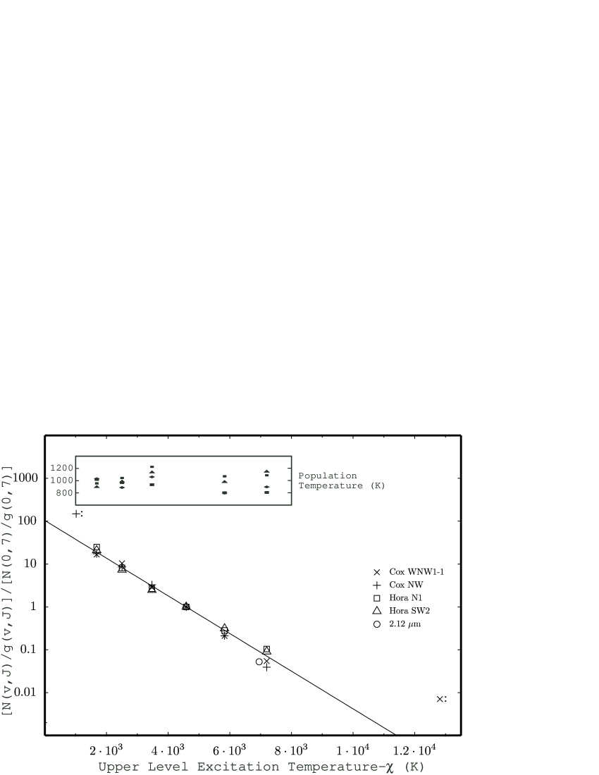
Figure 9.— The larger figure shows the population divided by the statistical weight in various $v,J$ states relative to that in the $v$=0,$J$=7 level (the origin of the 0-0 S(5) transition) as a function of the energy of the level expressed in units of the excitation temperature, as described in the text. The line shows the relation if all of the levels were characterized by a gas temperature of 988 K. The insert gives the gas temperature derived for each level, using the 0-0 S(5) line for reference and demonstrates the relatively small dispersion around the average temperature of 988 K. The +: indicates the position of the 0-0 S(1) line and the o the position of the 2.12 $\mu$m line, neither of which were used in deriving the best fit.

Table 2Relative Line Fluxes and Derived Temperatures for the H₂

		Relative Flux in Different Samples
		Cox	Cox	Hora	Hora	Full
Transition	$\chi$ (K)	WNW 1-1 S	NW	N	SW	Nebula
0-0 S(1)	1015	$\cdots$	$\cdots$	0.229:	$\cdots$
0-0 S(2)	1681	0.088	0.091	0.132	0.11
0-0 S(3)	2503	0.916	0.757	0.716	0.645
0-0 S(4)	3474	0.319	0.368	0.296	0.277
0-0 S(5)	4586	1	1	1	1
0-0 S(6)	5829	0.174	0.176	0.235	0.26
1-0 S(1)	6951	$\cdots$	$\cdots$	$\cdots$	$\cdots$	0.47
0-0 S(7)	7196	0.294	0.212	0.563	0.49
1-1 S(7)	12817	0.033:	$\cdots$	$\cdots$	$\cdots$
	$\rm Derived~{}T_{\mathrm{excit}}$	935	905	1040	1080
	standard deviation	110	98	109	97
	$\langle\rm Derived~{}T_{\mathrm{excit}}\rangle$	988
	standard deviation	119

4.3. Does the weakness of the H₂ 1-1 S(7) transition indicate that H₂  emission is powered by shocks?

H06 argues that the weakness of the 1-1 S(7) line shows that the H₂ emission must be shock excited rather than photo excited. Since their subsequent interpretation of the observed features of the nebula are based on this assumption, it merits critical examination. H06 state, without presenting detailed proof, that the 1-1 S(7) line is “normally strong” under photo excitation. They did not detect this line, but they did detect the nearby 0-0 S(7) line. Therefore, we base our discussion on the flux ratio of 1-1 S(7) to the 0-0 S(7) line. Examination of their spectra (H06 Figure 9) indicates that the flux ratio must be less than about 0.1. The 1-1 S(7) appears to be present in the Cox98 spectra at a level giving a line ratio of about 0.1.

Figure 10 shows the results for a series of calculations in which isothermal clouds with a range of temperatures and densities was exposed to the radiation field of the central star. The central star was approximated as a blackbody and the X-ray continua as a series of free-free emitters with the published luminosities and temperatures. The total continuum was attenuated by an effective column density of 10²² cm^-2 to approximate the extinction of the ionizing radiation by the H⁺ region. Typical planetary nebula abundances and ISM grains were assumed. The clouds had a thickness of $3\times 10^{15}$ cm. The figure shows the 1-1 S(7)/0-0 S(7) line ratio. The predicted ratio is generally quite small for the values of the H₂ density and temperature considered, approaching the upper limit that we identify above only at combinations of low H₂ density and temperature.

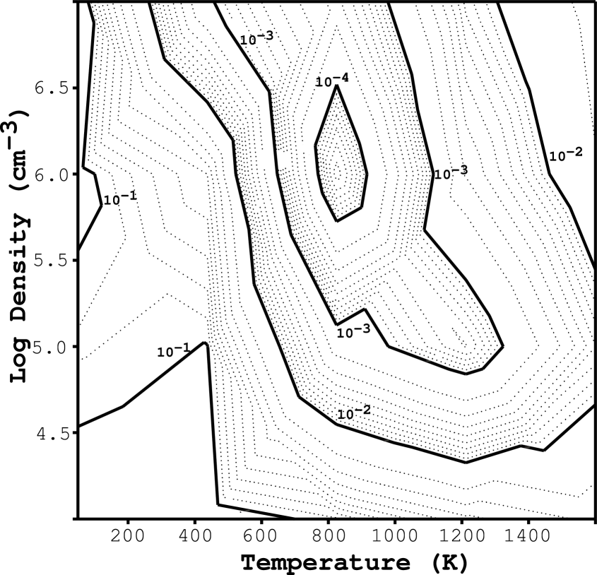
Figure 10.— This plot shows the expected flux ratio of the 1-1 S(7) and 0-0 S(7) lines as a function of the local temperature and density in the PDR.

Cox98 argue that the total density must exceed 10⁵ $\rm cm^{-3}$  in order for collisions to dominate and produce the closely single-temperature population distribution. This would be the density to combine with the derived temperature of 900 K for comparison with the S(7) line ratio, if the emitting zone were dominantly molecular hydrogen. In that case the predicted line ratio is much lower than the upper limit of the observations and one concludes that the observed weakness of the 0-0 S(7) line is not a useful indicator of the excitation mechanism as assumed by H06.

OHF05 derived a density of the molecular hydrogen from observations of the 2.12 $\mu$m line, finding a value of $6\times 10^{4}$ $\rm cm^{-3}$. However, they assume that the population of the level producing the transition was in LTE at 900 K, which seems to be the case as the upper state producing the 2.12 $\mu$m line falls right on the population distribution for this temperature. Using this density would also still indicate that the S(7) line ratio is not a useful indicator of the excitation mechanism. However, the challenge remains of explaining the unexpected combination of temperature and density.

Most of the existing calculations of H₂ population distributions and resulting emission spectra have been done for the case of a PDR near an HII region (Black & van Dishoeck 1987). The stellar radiation field of an O or B star peaks near the wavelengths that excite the electronic transitions of H₂, about 1000 Å. The main effect of illumination by this continuum is absorption into excited electronic states which then decay into excited vibration-rotation levels within the ground electronic state of H₂. A very non-thermal distribution is produced by these electronic photo excitations, as H06 points out.

However, the Cox98 and H06 spectra discussed in the preceding section show that the population distribution within lower levels of H₂ is well matched by a thermal distribution at about 900K. The non-thermal population distribution produced by O-star photo-excitation is simply not seen. This is not surprising since the environment is so dissimilar from that near a main sequence O or B star. The stellar radiation field of the Helix Nebula central star peaks at much shorter wavelengths than that of an O star, and § 4.1.2 shows that the observed stellar continuum in the 912-1100 Å interval is too small to account for the luminosity of the H₂ lines by photo-excitation, since the excitation of the fluorescent lines uses but a small fraction of the total energy in the 912-1100 Å interval. We agree with H06, that the pure rotational H₂ lines are not photon pumped, but not for the reasons they give. They are far too bright to be produced by photo-excitation by the current stellar continuum. We established in §  4 that the PDR’s of the knots almost certainly cannot be powered by shocks. Another energy source is needed.

4.4. The Nature of the Dissociation Front in the Knots

In § 4.1.1 and § 4.1.2 we examined the energy budget for the Helix Nebula, establishing that only the central star radiation more energetic than 13.6 eV (the extreme ultraviolet radiation or EUV) has enough power to drive the large total flux of H₂ emission that is observed, thus expanding upon and quantifying the conclusions in Cox98. This means that the soft X-ray heating processes and 912-1100 Å  (FUV) photo-excitation mechanisms (Natta & Hollenbach 1998) do not explain the Helix observations. The absence of a stellar wind and other time-scale considerations have already established (OHF05) that shocks cannot be powering the H₂ emission and in §  4.3 we showed why the justification of H06 for a shocks interpretation is incorrect. Although Phillips (2006) established a loose correlation between soft X-ray flux and H₂ emission, this correlation is probably secondary rather than primary, as there is insufficient X-ray emission to power the H₂ emission; but, the stars that are strong H₂ emitters have high temperatures, like the central star in the Helix Nebula. This means that these stars share the property of the EUV radiation being dominant over FUV radiation. Clearly a new process is required. Based on this observational foundation, we identify a new state of equilibrium that may be common, but has not previously been identified. A new mechanism utilizing the EUV radiation is briefly described here and will be elaborated upon in a future publication.

The ionized flows from the knots are advection dominated, meaning that recombinations are relatively unimportant (Henney 2001). As a result, neither the FUV or X-ray models (Hollenbach & Tielens 1997, Natta & Hollenbach 1998) is relevant to the dissociation fronts in the Helix knots. Instead, the dissociation front merges with the ionization front (Bertoldi & Draine 1996) and the dissociation of H₂ in this merged front is controlled by the ionizing EUV. The fact that neutral hydrogen 21 cm is not observed in the inner region of the Helix Nebula (Rodríguez et al. 2002) where the optically bright knots are found supports this model and the appearance of 21 cm emission from the more distant and fainter outer-ring knots indicates that a neutral hydrogen zone is only present there.

The low ionization parameter found in the Helix knots leads to substantial deviations from ionization and thermal equilibrium since the dynamical time is shorter than the ionization and heating times. The effects of this upon the emission from the ionized gas was discussed at length in OHF05. The dissociation of H₂ in such a front is predominantly due to chemical reactions with ionized species such as O⁺, and is therefore a strong function of the ionization fraction, which is determined by the absorption of EUV radiation. The radiation field is largely determined by the opacity in the fraction of hydrogen that is neutral, the key element being its determination of the amount of O⁺. It is the reaction of O⁺ with H₂ that destroys the H₂  rather than the much slower rate of photo-dissociation of H₂. This is essentially a one-way process, with H₂ entering the zone from the cold molecular core and being converted directly to H⁺. This transition zone is heated by the photo-ionization of neutral hydrogen and can be quite broad and the preliminary models indicate that it can produce warm H₂  column densities of about 10¹⁹ cm^-2, as required by the observations (OHF05). To the best of our knowledge, no models of such EUV-dominated dissociation regions have been calculated. We are calculating detailed models of such regions, which will be reported upon in a future paper and restrict ourselves here to this brief description.

It is likely that the same process determines the emission seen from the sheath of the tails in 2.12 $\mu$m. The first-order theory for shadowed columns behind optically thick knots was presented by Cantó et al. (1998). They illustrated that the shadowed regions are illuminated by LyC photons emitted from recombining hydrogen, that this radiation was closer to 13.6 eV than the ionizing stellar radiation, and that the flux density of these diffuse LyC photons was about 0.15 that of the direct LyC flux from the central star. These diffuse LyC photons are almost certainly the source of the heating of the H₂ in the tails as the surface brightness in 2.12 $\mu$m is about 0.23$\pm$0.08 that in the directly illuminated bright cusp (§ 3.6). The implausibility of shocks is also true here and the shortfall of energy from the FUV radiation is even greater than in the cusps because having a strong diffuse FUV radiation field would demand a large optical depth in dust for the nebula as a whole, which is not indicated by its emission line spectrum. A separate detailed H₂ model is required for the tail because the illuminating FUV will be of lower energy and the density much lower than in the bright cusp.

4.5. The Absence of Radial Features in the Center of the Helix Nebula

In a recent paper, Meaburn et al. (2005) presented the analysis of images made in the center of the Helix Nebula in H$\alpha$+[N II] in 1992 (technical details described in Meaburn et al. (1998). They present a high contrast rendering of the image (their Figure 10) and argue that radial “spokes” can be seen to faintly continue inside the boundary of the “cometary globules” to within about 30″ from the central star.

An arguably superior image of the region is available in the Cerro Tololo Interamerican Observatory 4-m MOSAIC images made in a similar filter (H$\alpha$+[NII]) and resolution, with a pixel scale (0.26″/pixel). The individual exposures were 300 s and in the central region, where the fields of the four different pointings overlap, the effective exposure was 1200 s. A straightforward examination of this image using various levels of brightness and contrast did not reveal the features posited by Meaburn et al. (O’Dell 2005). We have now more intensively examined the same images, by employing median filters of 20x20 pixels and 40x40 pixels and dividing the original images by these, a technique previously employed (OMM04) to enhance the visibility of radial features in the outer parts of the nebula. The results are shown in Figure 11 in negative depiction or the highly stretch range of intensities of 0.97-1.03. One sees no indication of radial features extending inside the radius at which the knots disappear. We argue that our images are a better test of such features since one can see numerous stars and galaxies that do not appear in the Meaburn et al. (2005) image.

This non-detection of such features, even only slightly inside the position of the easily visible bright cusp knots is a strong argument that this boundary indicates where knots were first formed and does not represent a boundary where knots have been destroyed. An attractive model for generating the initial irregularities that develop into the knots is presented in the calculations of García-Segura et al. (2006), who argue that these should arise at the boundary of shocked material as the initial fast-wind phase of the nebula ends, which is likely to be at about this position within the nebula.

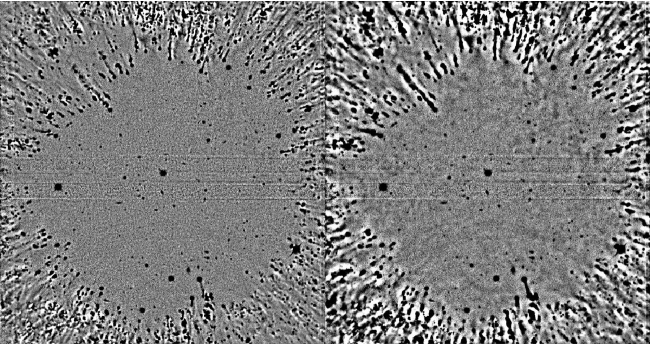
Figure 11.— This 377″x398″ H$\alpha$+[N II] image of the center of the Helix Nebula shows the ratio of the original image divided by a median filtered image of 20x20 pixels (left) and of 40x40 pixels (right). No indication of the inner region radial spoke features reported by Meaburn et al. (2005) are seen. The horizontal and vertical linear features are the seams of the mosaic formed from several CCD’s.

4.6. A Critique of Stream-Source Models for the Helix Knots

In a series of papers, Dyson and collaborators have developed a model for the structure of the Helix knots based on the hydrodynamic interaction that results when ionized gas is injected into a subsonic stream that flows past the injection source (Dyson et al. 1993, 2006).

Although the injected ionized gas is assumed to arise from an ionization front on the head of a neutral globule, the radiation transfer and ionization process is not explicitly included in the models. This makes it very difficult to make meaningful comparison between the results of these models and observations of the Helix nebula.

Our new H₂  observations clearly show (§ 3.2) that the limb-brightened edges of the knot tails correspond to an ionization front. Additionally, the width of the tail is equal to the width of the bright cusp at the head of the knot and its conic projection (O’Dell 2000). This would seem to conclusively establish that radiation shadowing, rather than hydrodynamic interactions, is the primary determinant of the structure of the tails. In the stream-source model, although tail widths are predicted to be of the same order as the width of the injection source, there is no reason to expect them to be equal, unless the parameters are fine-tuned.

The kinematic arguments given in support of the stream-source model (Meaburn et al. 2006) also do not stand up to close scrutiny. They are based on the ground-based echelle spectroscopic observations of Meaburn et al. (1998), which seem to show an acceleration of gas along the tail of the knot 378–801. However, a comparison with the much higher resolution HST observations (e.g., O’Dell et al. 2005, and also the image available at http://hubblesite.org/gallery/album/entire_collection/pr199613b). clearly shows that the sample regions used in that observational study all correspond to independent knots that are merely projected onto the tail of 378–801. Therefore, the observed variation in velocity does not represent an acceleration along the tail, but simply a tendency towards higher velocities in knots that are farther from the central star, which has already been noted from CO observations (Young et al. 1999).

5. Conclusions

We have been able to use existing and new observations to reach a number of important conclusions about the knots in the Helix Nebula.

1. There is sufficient energy to power the nebula’s H₂ emission only in extreme ultraviolet radiation from the central star with energies $\geq$13.6 eV, thus eliminating photo-excitation by the 912-1100 Å and X-ray flux that has been assumed in previous general models.

2. There is no evidence from infrared emission lines for shock excitation of the knots’ H₂ emission, the lack of a driving stellar wind and previous arguments of time-scale having come to the same conclusion.

3. Spectrophotometry of multiple lines in four sample regions and the total nebular flux ratio in the H₂ 0-0 S(5) and 2.12 $\mu$m lines indicates that the H₂ emitting zones are all about 988$\pm$119 K, closely resembling LTE.

4. The 2.12 $\mu$m emission from individual knots falls immediately inside the ionized gas zone traced by H$\alpha$ emission. This is true for both the bright cusps and their fainter tails, the latter establishing that the tails are primarily ionizing radiation shadows, rather than the result of purely hydrodynamic processes.

5. The advection dominated nature of the knot cusps means that there is no extended neutral hydrogen zone between the cold molecular knot core and the ionized gas layer. This zone of irradiation of H₂ by EUV photons is probably the region producing the observed hot gas in the cusps on the star-facing side of the molecular knots and the shadowed regions of the tails.

6. No evidence was found for knots within the He II core nor were earlier claims verified of linear features extending nearly in to the central star, arguing that the knots have only been created outside the high ionization core.

References

- Bertoldi & Draine (1996) Bertoldi, F., & Draine, B. T. 1996, ApJ, 458, 222
- (2) Black. J. H., & van Dishoek, E. F. 1987, ApJ, 322, 412
- Bohlin et al. (1982) Bohlin, R. C., Harrington, J. P., & Stecher, T. P. 1982, ApJ, 252, 635
- Burkert & O’Dell (1998) Burkert, A., & O’Dell, C. R. 1998, ApJ, 503, 792
- Cantó et al. (1998) Cantó, J, Raga, A., Steffen, W., & Shapiro, P. R. 1998, ApJ, 5002, 695
- (6) Cerruti-Sola, M., & Perinotto, M. 1985, ApJ, 291, 237
- Cox et al. (1998) Cox, P., Boulanger, F., Huggins, P. J., Tielens, A. G. G. M., Forveille, T., Bachiller, R., Cesarsky, D., Jones, A. P., Young, K., Roelfsema, P. R., & Cernicharo, J. 1998, ApJ, 495, L23 (Cox98)
- Dabrowski (1984) Dabrowski, I. 1984, Canadian J. Phys., 62, 1639
- Dyson et al. (1993) Dyson, J. E., Hartquist, T. W., & Biro, S., 1993, MNRAS, 261, 430
- Dyson et al. (2006) Dyson, J. E., Pittard, J. M., Meaburn, J., & Falle, S. A. E. G. 2006, A&A, 457, 561
- Fazio et al. (2004) Fazio, G. et al. 2004, ApJS, 154, 10
- Garcia Segura et al. (2006) García-Segura, G., López, J. A., Steffen, W., Meaburn, J., & Manchado, A. 2006, ApJ, in press
- Gonzaga et al. (2005) Gonzaga, S., et al. 2005, ACS Instrument Handbook, Version 6.0, (Baltimore:STScI)
- Guerrero et al. (2001) Guerrero, M. A., Chu, Y.-H., Gruendl, R. A., Williams, R. M., & Kaler, J. B. 2001, ApJ, 553, L55
- Harris et al. (2007) Harris, H. C., Dahn, C. C., Canzian, B., Guetter, H. H., Leggett, S. K., Levine, S. E., Luginbuhl, C. B., Monet, A. K. B., Monet, D. G., Pier, J. R., Stone, R. C., Tilleman, T., Vrba, F. J., & Walker, R. L. 2007, AJ, in press
- Henney (2001) Henney, W. J. 2001, RMxAC, 10, 57
- Hollenbach & Tielens (1997) Hollenbach, D. J., & Tielens, A. G. G. M. 1997, ARAA, 35, 179
- Hora et al. (2006) Hora, J. L., Latter, W. B., Smith, H. A., & Marengo, M. 2006, ApJ, in press (H06)
- Holtzman et al. (1995) Holtzman, J. A., Burrows, C. J., Castertano. S., Hester, J. J., Trauger, J. T., Watson, A. M., & Worthey, G. 1995, PASP, 107, 1065
- Houck et al. (2004) Houck, J. R. et al. 2004, ApJS, 154, 18
- Huggins et al. (2002) Huggins, P. J., Forveille, T., Bachiller, R., Cox, P., Ageorges, N., & Walsh, J. R. 2002, ApJ, 573, L55.
- Lopez-Martin et al. (2001) López-Martín, L., Raga, A. C., Melleman, G., Henney, W. J., & Cantó, J. 2001, ApJ, 548, 288
- Leahy et al. (1994) Leahy, D. A., Zhang, C. Y., & Kwok, S. 1994, ApJ, 422, 205
- Leahy et al. (1996) Leahy, D. A., Zhang, C. Y., Volk, K., & Kwok, S. 1996, ApJ, 466, 352
- Meaburn et al. (2005) Meaburn, J., Boumis, P., López, J. A., Harman, D. J., Bryce, M., Redman, M. P., & Mavromatakis, F. 2005, MNRAS, 360, 963 M05
- Meaburn et al. (1998) Meaburn, J., Clayton, C. A., Bryce, M., Walsh, J. R., Holloway, A. J., & Steffen, W. 1998, MNRAS, 294, 201
- Meaburn et al. (1992) Meaburn, J., Walsh, J. R., Clegg, R. E. S., Walton, N. A., & Taylor, D. 1992, MNRAS, 255, 177
- Meixner et al. (2004) Meixner, M., McCullough, P., Hartman, J., O’Dell, C. R., & Speck, A. K. 2004, in ASP Conf. Ser. 313, Asymmetrical Planetary Nebulae III: Winds, Structure, and the Thunderbird, ed. M. Meixner et al. (San Francisco: ASP), 234
- Meixner et al. (2005) Meixner, M., McCullough, P. R., Haartman, J., Son, M., & Speck, A. K. 2005, AJ, 130, 1784 (MX05)
- Mellema et al. (1998) Mellema, G., Raga, A. C., Cantó, J., Lundqvist, P., Balick, B., Steffen, W., & Noriega-Crespo, A. 1998, A&A, 331, 335
- Natta & Hollenbach (1998) Natta, A., & Hollenbach, D. 1998, A&A, 337, 517
- O’Dell (1998) O’Dell, C. R. 1998, AJ, 116, 1346
- O’Dell (2000) O’Dell, C. R. 2000, AJ, 119, 2311
- O’Dell (2004) O’Dell, C. R. 2004, PASP, 116, 729
- O’Dell (2005) O’Dell, C. R. 2005 RMxAC, 23, 5
- O’Dell et al. (2002) O’Dell, C. R., Balick, B., Hajian, A. R., & Henney, W. J. 2002, AJ, 123, 3329
- O’Dell & Burkert (1997) O’Dell, C. R., & Burkert, A. 1997, in IAU Symp. 180, 332
- O’Dell & Doi (1999) O’Dell, C. R., & Doi, T. 1999, PASP, 111, 1316 Planetary Nebulae, ed. H. J. Habing & H. J. G. L. M. Lambers (Dordrecht: Kluwer), 332
- O’Dell & Handron (1996) O’Dell, C. R., & Handron, K. D. 1996, AJ, 111, 1630
- O’Dell et al. (2000) O’Dell, C. R., Henney, W. J., & Burkert, A. 2000, AJ, 119, 2910 (OHB00)
- O’Dell et al. (2005) O’Dell, C. R., Henney, W. J., & Ferland, G. J. 2005, AJ, 130, 172 (OHF05)
- O’Dell et al. (2004) O’Dell, C. R., McCullough, P. R., & Meixner, M. 2004, AJ, 128, 2339 (OMM04)
- Phillips (2006) Phillips, J. P. 2006, MNRAS, 368, 819
- Rauch (2003) Rauch, T. 2003, A&A, 403, 709
- Rodriguez et al. (2002) Rodríguez, L. F., Goss, W. M., & Williams, R. 2002, ApJ, 574, 179
- Shaw et al. (2005) Shaw, G., Ferland, G. J., Abel, N.P., Stancil, P. C., & van Hoof, P. A. M. 2005, ApJ, 624, 794
- (47) Speck, A. K., Meixner, M., Fong, D., McCulough, P. R., Moser, D. E., & Ueta, T. 2002, AJ, 123, 346
- Thompson et al. (1998) Thompson, R. I., Rieke, M., Schneider, G., Hines, D. C., & Corbin, M. R. 1998, ApJ, 492, L95
- Walsh & Ageorges (2004) Walsh, J. R., & Ageorges, N. 2004, in IAU Symp. 209 Planetary Nebulae: Their Evolution and Role in the Universe, eds. S. Kwok, M. Dopita, & R. Sutherland, 275
- (50) Wolniewicz, L., Simbotin, I., & Dalgarno, A. 1998, ApJS, 115, 293
- Wood et al. (2004) Wood, K., Mathis, J. S., & Ercolano, B. 2004, MNRAS, 348, 1337
- (52) Young, K., Cox, P., Huggins, P. J., Forveille, T., & Bachiller, R. 1999, ApJ, 522, 387