Pre-Merger Localization of Gravitational-Wave Standard Sirens With LISA:
Harmonic Mode Decomposition

Abstract

The continuous improvement in localization errors (sky position and distance) in real time as LISA observes the gradual inspiral of a supermassive black hole (SMBH) binary can be of great help in identifying any prompt electromagnetic counterpart associated with the merger. We develop a new method, based on a Fourier decomposition of the time-dependent, LISA-modulated gravitational-wave signal, to study this intricate problem. The method is faster than standard Monte Carlo simulations by orders of magnitude. By surveying the parameter space of potential LISA sources, we find that counterparts to SMBH binary mergers with total mass $M\sim 10^{5}$–$10^{7}\mathrm{M}_{\odot}$ and redshifts $z\mathrel{\hbox to0.0pt{\lower 4.0pt\hbox{\hskip 1.0pt$\sim$}\hss}\raise 1.0pt\hbox{$<$}}3$ can be localized to within the field of view of astronomical instruments ($\sim\deg^{2}$) typically hours to weeks prior to coalescence. This will allow a triggered search for variable electromagnetic counterparts as the merger proceeds, as well as monitoring of the most energetic coalescence phase. A rich set of astrophysical and cosmological applications would emerge from the identification of electromagnetic counterparts to these gravitational-wave standard sirens.

I Introduction

One of the key objectives of the planned, low-frequency gravitational-wave (GW) detector LISA (Laser Interferometric Space Antenna) is the detection of supermassive black hole (SMBH) binary mergers at cosmological distances. The observation of these chirping GW sources would deepen our understanding of (i) general relativity, e.g. by offering unique tests of spacetime physics in the vicinity of SMBHs dre04 ; mil05 ; hm05 ; bcw06 ; aru06 , (ii) cosmology, by providing additional constraints on the luminosity distance–redshift relation sch86 ; hug02 ; hh05 , (iii) large-scale structure, by indirectly constraining hierarchical structure formation scenarios bbr80 ; bh92 ; mhn01 ; bbw05 , and (iv) black hole astrophysics, e.g. by allowing accurate determinations of Eddington ratios, and other attributes of black hole accretion, in systems with SMBH mass and spin known independently, from the GW measurements mp05 ; koc06 ; dot06 .

From a purely astronomical point of view, one of the most attractive features of the LISA mission design is the possibility to constrain the 3-dimensional location (i.e. sky position and distance) of GW inspiral sources to within a small enough volume that the identification of potential electromagnetic (EM) counterparts to SMBH merger events can be contemplated seriously. Indeed, the accuracy of such LISA localizations at merger are encouraging, with an error volume $\delta\Omega\times\delta z=0.3\deg^{2}\times 0.1$ for SMBH masses $m_{1}=m_{2}=10^{6}\mathrm{M}_{\odot}$ at $z=1$, for instance vec04 . In Ref. koc06 , we have shown that this accuracy may be sufficient to allow an unique identification of the bright quasar activity that may be associated with any such SMBH merger.

Another possibility, examined here in detail, is to monitor the sky for EM counterparts in real time, as the SMBH inspiral proceeds. This is arguably one of the most efficient ways to identify reliably (prompt) EM counterparts to SMBH merger events, since the exact nature of such counterparts is a priori unknown. Using the GW inspiral signal accumulated up to some look–back time, $t_{\mathrm{f}}$, preceding the final coalescence, one already has a partial knowledge of where the source of GWs is located on the sky. Since the sky position is deduced primarily from the detector’s motion around the Sun, one anticipates that angular positioning uncertainties will not change too dramatically during the last few days before merger, so that a targeted EM observation of the final stages of inspiral may be a feasible task. Here, we present an in-depth study of the potential for such pre-merger localizations with LISA, while we discuss various astrophysical concepts and observational strategies for EM counterpart identifications in a companion work paper2 .

The main purpose of the present analysis is thus to determine the accuracy of SMBH inspiral localizations with LISA, as a function of look–back time, $t_{\mathrm{f}}$, prior to merger. The LISA detector is not uniformly sensitive to sources with different sky positions and angular momentum orientations. Results will thus generally depend on the fiducial values of these angles. Our first objective is to calculate the time-dependence of distributions of localization errors, for randomly oriented sources, over a large range of values for the SMBH masses and source redshift. A second objective of our analysis is to estimate source parameter dependencies for these distributions of localization errors, i.e. how the 3-dimensional (sky position and distance) localization error distributions depend on the fiducial sky position of GW sources. This is useful to understand which regions of the sky may be best suited for the identification of EM counterparts to SMBH merger events. To the best of our knowledge, this angle dependence has not been explored in detail before, not even in terms of final errors at ISCO (i.e. at $t_{\mathrm{f}}=t_{\rm isco}$, when using the complete inspiral data-stream, up to the innermost stable circular orbit, or ISCO).

Parameter estimation uncertainties for LISA inspirals have been considered previously, under a variety of approximations cut98 ; mh02 ; hug02 ; bc04 ; vec04 ; bbw05 ; hh05 ; aru06 ; lh06 . These studies differ in the levels of approximation adopted for the GW waveform, using various orders of the post-Newtonian expansion. The LISA signal output for these waveforms are obtained through a linear combination of the two GW polarizations, $h_{+}(t)$ and $h_{\times}(t)$, with the beam pattern functions, $F_{+}$ and $F_{\times}$. The beam patterns define the detector sensitivity for the two polarizations. They are determined by the angles describing the instantaneous orientation of the LISA constellation relative to the GW polarizations. As the LISA detector constellation orbits the Sun, with a one year period, $F_{+}$ and $F_{\times}$ are slowly changing in time and this introduces an additional time dependence in the LISA signal. As first shown by Cutler cut98 , the source sky position can be determined with LISA using this modulation. In the formalism given by Cutler cut98 , this modulation couples time and angular dependencies in a complicated way, making the estimation of localization errors numerically costly for a large set of SMBH binary random orientations and parameters.

Using a different approach, Cornish & Rubbo cr03 have derived the orbital modulation in a much simpler form, in which the angular parameter dependence and the time dependence can be decoupled. Here, starting directly from the original Cutler cut98 expression, we give an independent derivation of the Cornish & Rubbo cr03 formula and write it in an equivalent form, from which decoupling is more evident. We do this by expanding the LISA response function into a discrete Fourier sum of harmonics of the fundamental frequency of LISA’s orbital motion, $f_{\oplus}=1\,\mathrm{yr}^{-1}$. Since LISA’s orbit does not include high frequency features, we expect this sum to be quickly convergent. In fact, it is clear from the Cornish & Rubbo cr03 result that the expansion terminates at $4f_{\oplus}$ and that there are no higher order harmonics due to the detector’s motion. The series coefficients in the expansion are independent of time and only depend on the relative angles at ISCO. We then develop a Fisher matrix formalism in which parameter error distributions can be mapped independently of time, while the time dependence can be computed independently of the specific SMBH binary orbital elements. A Monte Carlo simulation for random binary orientations then becomes a simple linear combination, without any integral evaluations. This greatly reduces the numerical cost of estimating parameter uncertainty distributions, even at fixed observation time (e.g. to map distributions of errors at ISCO). We use this numerical cost advantage

1. to map the distribution of localization errors for the full three dimensional grid of SMBH total mass ($M=10^{5}$–$10^{8}\mathrm{M}_{\odot}$), redshift ($z=0.1$–$7$) and arbitrary look–back time ($t_{\mathrm{f}}$) before merger,

2. to study how source localization error distributions vary systematically with sky position, and

3. to discuss implications, in terms of advance warning times, for prompt electromagnetic counterpart searches with large field-of-view astronomical instruments.

We call this new approach the harmonic mode decomposition (HMD). The method verifies that the amplitude modulation, which is restricted to frequencies less than $4f_{\oplus}=1.3\times 10^{-7}\,\mathrm{Hz}$, is indeed a very slow modulation when compared to the GW frequency of LISA SMBH inspirals ($0.03\,\mathrm{mHz}$–$1\,\mathrm{Hz}$). One plausibly expects that physical parameters which determine the amplitude modulation (like the source sky position and orbital inclination relative to the detector) can be estimated independently of the parameters which determine the GW frequency (like masses, orbital phase, time to ISCO). In the HMD method, the two sets of parameters are naturally separated and can be estimated independently. In particular, parameters related to the modulation can essentially be determined on a background of GW-cycle averaged signal. In the present work, we compute LISA inspiral localization errors with the approximation that high frequency signal parameters have strictly no cross-correlations with parameters related to the slow orbital modulation. In addition to the numerical advantages mentioned above, the HMD formalism offers a clear interpretation of the time evolution of uncertainties for the slow modulation parameters. This can be used to gain a better understanding of the general evolutionary properties of localization errors. The following questions, that we address in detail in our work, are particularly relevant.

1. Under what conditions do the localization uncertainties scale simply with the measured signal–to–noise ratio, and how do these uncertainties evolve during the final stages of inspiral?

2. To what extent do the high and low frequency signal parameters decouple?

3. What are the best determined combinations of the angular parameters?

4. How and why does the shape of the 3D localization error ellipsoid change during the final week(s) of observation?

In our analysis, we neglect the “Doppler phase” due to LISA’s orbital motion, SMBH spin precession effects and any finite SMBH binary orbital eccentricities. These approximations are advantageous for the resulting simplicity, but the use of the HMD method is not restricted to these approximations. We also outline a generalized HMD method which remains numerically much more efficient than standard methods. We leave a numerical implementation of this general HMD method to future work. It will be particularly interesting to determine how our approximate results for the evolution of LISA localization errors are modified when spin precession effects are included, since spin precession effects were shown to improve the final localization errors by factors of $3$–$5$ at ISCO vec04 ; lh06 .

The remainder of this paper is organized as follows. In § II we define our conventions and the assumptions made in our analysis. In § III we expand the LISA GW signal in Fourier modes and obtain the conversion from actual physical parameters to corresponding Fourier amplitudes. In § IV, we incorporate these results into a Fisher matrix formalism and derive the expressions necessary to estimate correlation errors for HMD signals. In § V, we quantify the computational advantages of the HMD method. In § VI, we present results from Monte Carlo computations of the time evolution of localization errors and discuss results in terms of advance warning times for prompt electromagnetic counterpart searches. In § VII, we develop toy models to interpret the time-dependence of LISA localization errors and to answer questions (i)–(iv) above. We summarize our results and conclude in § VIII.

II Assumptions and Conventions

This section is divided into three parts. First, we list the definitions of physical quantities used in this paper, in particular the variables describing a SMBH inspiral. Second, we give the equations which determine the LISA inspiral signal. Third, we state all the assumptions made in this work.

II.1 Definitions

In general, an SMBH inspiral is described by a total of 17 parameters. These include 2 redshifted mass parameters, $(\mathcal{M}_{z},\eta_{z})$, 6 parameters related to the BH spin vectors, ${\bm{p}}_{\mathrm{spin}}$, the orbital eccentricity, $e$, the source luminosity distance, $d_{\rm L}$, 2 angles locating the source in the sky, $(\theta_{N},\phi_{N})$, 2 angles that describe the relative orientation of the binary orbit, $(\theta_{NL},\phi_{NL})$, a reference time, $t_{\rm merger}$, and a reference phase at ISCO, $\phi_{\rm ISCO}$, and the orbital phase, $\phi_{\rm orb}$. Throughout this work, we restrict ourselves to circular orbits by omitting the orbital eccentricity, $e$, and instead of the orbital phase, $\phi_{\rm orb}$, we use the look–back time before merger, $t$, as our evolutionary time parameter. The LISA signal for a GW inspiral is determined by the above set of parameters and two additional angular parameters describing the orientation of LISA, $(\Xi,\Phi)$. We elaborate on the definitions of our mass and angular parameters below.

II.1.1 Mass Parameters

For component masses $m_{1}$ and $m_{2}$, the total mass is $M=m_{1}+m_{2}$, the reduced mass is $\mu=m_{1}m_{2}/M$, the symmetric mass ratio is $\eta=\mu/M$ and the chirp mass is defined as $\mathcal{M}=M\eta^{3/5}$ Gravitation . Throughout this work, we use geometrical units: ${\rm G}\equiv{\rm c}\equiv 1$. In this case, the mass can be expressed in units of time: $10^{6}\mathrm{M}_{\odot}\equiv 4.95\sec$. The measured GW waveforms are insensitive to the cosmological parameters, if they are expressed in terms of the luminosity distance and the redshifted mass parameters, e.g. $m_{z}=(1+z)m$ (same for redshifted chirp and reduced masses).

II.1.2 Time Parameters

We write a generic look–back time (or “observation time”) before merger as $t$, and a generic redshifted GW frequency (or “observation frequency”) as $f$. We use the leading order (i.e. Newtonian) approximation for the frequency evolution. Therefore, the observed frequency at look–back time $t$ before merger is (e.g. eq. 3.3 in ref. pw95 )

$$f_{0}(\mathcal{M}_{z},t) =\frac{5^{3/8}}{8\pi}t^{-3/8}\mathcal{M}_{z}^{-5/8},$$

$$=2.7\times 10^{-4}\,\mathrm{Hz}\left(\frac{t}{\rm day}\right)^{-3/8}\eta_{0.25}^{-3/8}M_{6z}^{-5/8},$$ (1)

or equivalently

$$t_{0}(\mathcal{M}_{z},f) =5(8\pi f)^{-8/3}\mathcal{M}_{z}^{-5/3}$$

$$=6.7{\,\rm min}\left(\frac{f}{f_{c}}\right)^{-8/3}\eta_{0.25}^{-1}M_{6z}^{-5/3},$$ (2)

where $M_{6z}$ is the redshifted total mass in units of $4\times 10^{6}\mathrm{M}_{\odot}$, $\eta_{0.25}=\eta/0.25$ is the symmetric mass ratio ($\eta_{0.25}=1$ for equal component masses, § II.3), $f_{c}={\rm c}/{\rm R}_{\oplus}=c/(1\,\mathrm{AU})=2.00\,\mathrm{mHz}$ is the inverse light-travel time across the radius of the LISA orbit, and the null index stands for the order of approximation. The inspiral phase extends until the innermost stable circular orbit (ISCO), at $6M$, is reached

$$f\leq f_{\rm ISCO} = 6^{-3/2}\pi^{-1}M_{z}^{-1}=1.1\,\mathrm{mHz}\times M_{6z}^{-1},$$ (3)

$$t\geq t_{\rm ISCO} = 5(3/2)^{4}\eta^{-1}M_{z}=33{\,\rm min}\times\eta_{0.25}^{-1}M_{6z}.$$ (4)

where $t_{\rm ISCO}$ is the (observer-frame) look–back time before merger corresponding to the ISCO, and $f_{\rm ISCO}$ is the (observer-frame) frequency at ISCO.

In the present work, we fix the start of the observation (i.e. when the source first enters LISA’s frequency band) at look–back time $t_{\mathrm{i}}$, and examine how the value of an end-of-observation time, $t_{\mathrm{f}}$, prior to merger affects the precision on source localization. We restrict ourselves to pre-ISCO inspiral signals, corresponding to $t_{\mathrm{f}}\geq t_{\rm ISCO}$. Note that any instantaneous look–back time $t$ associated with an observation lasting from look–back times $t_{\mathrm{i}}$ to $t_{\mathrm{f}}$ must obey $t_{\rm ISCO}\leq t_{\mathrm{f}}\leq t\leq t_{\mathrm{i}}$ in our notation.

II.1.3 Angular Parameters

LISA is an equilateral triangle-shaped interferometer with an arm-length of $5\times 10^{6}\,$km, orbiting around the Sun. The constellation trails $20^{\circ}$ behind the Earth and is tilted $60^{\circ}$ relative to the ecliptic. The detector plane precesses around the orbital axis with the same one-year period as the orbital period Danz04 .

Following closely Refs. cut98 and vec04 , including in notation, we define two coordinate systems. The barycentric frame is tied to the ecliptic, with ${\bf\hat{x}},{\bf\hat{y}}$ lying in the ecliptic plane and $\bf\hat{z}$ normal to it. The detector reference frame tied to the detector, with ${\bf\hat{z}^{\prime}}$ normal to the detector plane, while ${\bf\hat{x}^{\prime}},{\bf\hat{y}^{\prime}}$ are in the plane and co-rotating with the detector so that the arms are described by time-independent vectors. We refer to the barycentric frame with normal coordinates and to the detector frame with primed coordinates. The unit vectors defining the source location on the sky, ${\bf\hat{N}}$, and the SMBH binary orbital angular momentum, ${\bf\hat{L}}$, are described by polar angles $(\theta_{N},\phi_{N})$ and $(\theta_{L},\phi_{L})$ in the ecliptic frame, $(\theta^{\prime}_{N},\phi^{\prime}_{N})$ and $(\theta^{\prime}_{L},\phi^{\prime}_{L})$ in the detector frame:

$${\bf\hat{N}}(\theta_{N},\phi_{N}) ={\bf\hat{z}}\cos\theta_{N}+{\bf\hat{x}}\sin\theta_{N}\cos\phi_{N}+{\bf\hat{y}}\sin\theta_{N}\sin\phi_{N},$$ (5)

$${\bf\hat{L}}(\theta_{L},\phi_{L}) ={\bf\hat{z}}\cos\theta_{L}+{\bf\hat{x}}\sin\theta_{L}\cos\phi_{L}+{\bf\hat{y}}\sin\theta_{L}\sin\phi_{L}.$$ (6)

Since we assume no SMBH spins, orbital angular momentum is conserved and the $(\theta_{N},\phi_{N},\theta_{L},\phi_{L})$ coordinates are time-independent properties of the sources.

Let $(\Xi,\Phi)$ be the two angles specifying the orientation of the LISA system in the ecliptic: $\Phi$ describes its orbital phase during its motion around the Sun, while $\Xi$ describes the rotation of the triangle around its geometrical center. If their values at merger are written $\Xi_{0}$ and $\Phi_{0}$, then at an arbitrary look–back time $t$:

$$\Xi(t) = \Xi_{0}-\omega_{\oplus}t,$$ (7)

$$\Phi(t) = \Phi_{0}-\omega_{\oplus}t,$$ (8)

where $\omega_{\oplus}\equiv 2\pi/\,\mathrm{yr}$ is the orbital angular velocity around the Sun.

The time dependence of the detector normal vector $\bf\hat{z}^{\prime}$ can be expressed as

$${\bf\hat{z}^{\prime}}=\frac{1}{2}{\bf\hat{z}}-\frac{\sqrt{3}}{2}{\bf\hat{x}}\cos\Phi-\frac{\sqrt{3}}{2}{\bf\hat{y}}\sin\Phi.$$ (9)

The detector angles are given by

$$\cos\theta^{\prime}_{N} =\frac{1}{2}\cos\theta_{N}-\frac{\sqrt{3}}{2}\sin\theta_{N}\cos(\Phi-\phi_{N}),$$ (10)

$$\phi^{\prime}_{N} =\Xi+\tan^{-1}\left[\frac{\frac{\sqrt{3}}{2}\cos\theta_{N}+\frac{1}{2}\sin\theta_{N}\sin(\Phi-\phi_{N})}{\sin\theta_{N}\sin(\Phi-\phi_{N})}\right].$$ (11)

Let us also define $\psi^{\prime}$, the polarization angle of the GW waveform, as vec04

$$\tan\psi^{\prime}=\frac{{\bf\hat{L}}\cdot{\bf\hat{z}^{\prime}}-({\bf\hat{L}}\cdot{\bf\hat{N}})({\bf\hat{z}^{\prime}}\cdot{\bf\hat{N}})}{{\bf\hat{N}}\cdot({\bf\hat{L}}\times{\bf\hat{z}^{\prime}})}.$$ (12)

Note that there are only 6 independent angular parameters $(\theta_{N},\phi_{N},\theta_{L},\phi_{L},\Xi,\Phi)$. Other detector specific quantities like $\theta^{\prime}_{N}$, $\phi^{\prime}_{N}$, $\theta^{\prime}_{L}$, $\phi^{\prime}_{L}$, and $\psi^{\prime}$ can be expressed in terms of these 6 independent parameters using eqs. (5–12).

Let us introduce a new set of 6 independent angles,

$$\Omega=(\theta_{N},\phi_{N},\theta_{NL},\phi_{NL},\alpha,\gamma),$$ (13)

with the following definitions:

• $\theta_{NL}$ is the relative latitude of $\bf\hat{L}$ and $\bf\hat{N}$ (i.e. the inclination of the binary orbit to the line of sight),

• $\phi_{NL}$ is the relative longitude of $\bf\hat{L}$ and $\bf\hat{N}$,

• $\alpha\equiv\Xi-\Phi+\phi_{N}-\frac{3\pi}{4}$,

• $\gamma(t)\equiv\Phi(t)-\phi_{N}$.

The explicit definitions are given in Appendix B.

Let us refer to the angles at the reference time $t=t_{\rm merger}=0$ as $\Omega(0)$. Although $\Phi\equiv\Phi(t)$ and $\Xi\equiv\Xi(t)$ are time-dependent, as given by (7,8) $\alpha$ is a time-independent combination, unlike the time-dependent $\gamma\equiv\gamma(t)$. The angles at $t=0$ are thus given by $\Omega(0)=(\theta_{N},\phi_{N},\theta_{NL},\phi_{NL},\alpha,\gamma_{0})$.

These angles have the interesting property that they possess isotropic a priori distributions, like the original $\Omega(0)$ variables, but the measured GW waveforms expressed in terms of these new variables are much simpler than when they are expressed in terms of the original set eqs. (5–12).

Two additional quantities which are useful to describe the sensitivity of the detector in various directions are the antenna beam patterns cut98 :

$$F_{\times,+}(\Omega)= \frac{1+\cos^{2}\theta^{\prime}_{N}}{2}\cos 2\phi^{\prime}_{N}\cos 2\psi^{\prime}_{N}$$

$$\;\pm\cos\theta^{\prime}_{N}\sin 2\phi^{\prime}_{N}\sin 2\psi^{\prime}_{N},$$ (14)

where the sign $\pm$ is defined to be positive for $F_{\times}$, and negative for $F_{+}$. Equation (II.1.3) and the transformation rules eqs. (5–12) define the time evolution of the antenna beam patterns for a given set of final angles $\Omega(0)$ as the LISA system orbits around the Sun. Note that the LISA system is equivalent to two independent orthogonal-arm interferometers which are rotated by $45^{\circ}$ relative to each other cut98 . Both data-streams are given by the same equations (see eq. [21] below), modulo a change of one of the angles for the second detector: ${\phi^{\prime}}^{\rm II}_{N}={\phi^{\prime}}^{\rm I}_{N}-\pi/4$ (or equivalently $\alpha^{\rm II}=\alpha^{\rm I}-\pi/4$ using our time-independent angular variables). Thanks to this simple relationship between the two data-streams, it is possible to carry out all the calculations for the first data-stream, and later include the second data-stream in the final expression by varying the fiducial angle $\alpha$.

II.1.4 Grouping the Parameters

We group the most important parameters describing the inspiral as follows:

$${\bm{p}}_{\mathrm{slow}} \equiv \{d_{\rm L},\Omega\},$$ (15)

$${\bm{p}}_{\mathrm{fast}} \equiv \{\mathcal{M}_{z},\mu_{z},t_{\rm merger},\phi_{\rm ISCO}\},$$ (16)

$${\bm{p}}_{\mathrm{spin}} \equiv \{2~{}\rm{spin~{}magnitudes},4~{}\rm{spin~{}angles}\}.$$ (17)

This organization of parameters has fundamental importance in our formalism. As we show in § II.2, the parameters ${\bm{p}}_{\mathrm{fast}}$ and ${\bm{p}}_{\mathrm{spin}}$ relate to the high frequency GW signal, while the parameters ${\bm{p}}_{\mathrm{slow}}$ relate to the distinctly slow orbital modulation.

II.2 LISA Inspiral Signal Waveform

For a circular binary inspiral, the two polarizations of GW signal are well approximated by the restricted post-Newtonian expressions

$$h_{+}(t) = 2\frac{{\cal M}^{5/3}(\pi f)^{2/3}}{d_{\rm L}}(1+\cos^{2}\theta_{NL})\cos\phi_{\rm GW}(t),$$ (18)

$$h_{\times}(t) = -4\frac{{\cal M}^{5/3}(\pi f)^{2/3}}{d_{\rm L}}\cos\theta_{NL}\sin\phi_{\rm GW}(t).$$ (19)

The GW phase $\phi_{\rm GW}(t)\equiv\phi_{\rm GW}({\bm{p}}_{\mathrm{fast}},{\bm{p}}_{\mathrm{spin}};t)$, which is twice the orbital phase , $\phi(t)=2\phi_{\rm orb}(t)$, can be expanded into the series

$$\phi_{\rm GW}({\bm{p}}_{\mathrm{fast}},{\bm{p}}_{\mathrm{spin}};t)\approx \phi_{\rm ISCO}+\phi_{0}(\mathcal{M}_{z};t)+\phi_{1}(\mathcal{M}_{z},\mu_{z};t)$$

$$+\phi_{2}(\mathcal{M}_{z},\mu_{z},{\bm{p}}_{\mathrm{spin}};t)+\dots,$$ (20)

where $\phi_{0}(\mathcal{M}_{z};t)$ is the leading order Newtonian solution to the phase evolution, successive terms correspond to small general relativistic corrections, $\phi_{\rm ISCO}$ is the reference phase at ISCO and $\phi_{n}(t_{\rm ISCO})=0$ for all $n\geq 0$. The instantaneous GW frequency is defined as the time derivative of the GW phase (20), i.e. $f=f(t)\equiv\mathrm{d}\phi_{\rm GW}/\mathrm{d}t$, which changes very slowly compared to the GW phase itself, $\phi_{\rm GW}(t)$. In practice we use the Newtonian approximation (1), $f_{0}(t)=\mathrm{d}\phi_{0}/\mathrm{d}t$. Note that equation (20) depends implicitly on the reference time, $t_{\rm merger}$, since our time variable $t$ is the look–back time before $t_{\rm merger}$ (see § II.1.2)

The signal measured by LISA is a linear combination of the two polarizations (18), weighted by the antenna beam patterns $F_{+}^{\rm I,II}$ and $F_{\times}^{\rm I,II}$ for each of the two equivalent interferometers, defined by (II.1.3), resulting in the two observable data–streams

$$h^{\rm I,II}(t)=\frac{\sqrt{3}}{2}[F_{+}^{\rm I,II}h_{+}(t)+F_{\times}^{\rm I,II}h_{\times}(t)],$$ (21)

where the factor $\sqrt{3}/2=\sin(60^{\circ})$ comes from the opening angle of the LISA arms. The beam patterns are determined by the relative orientation of the source polarizations and the detector. Their time-dependence is due to the following three main effects: LISA changes its orientation as it orbits the Sun, LISA changes its relative distance to the source as it orbits the Sun, and the orbital plane of the SMBH binary can precess because of spin-orbit coupling effects. Substituting (18) in (21) and expressing it in complex form, we get

$$h^{\rm I,II}(t)=\frac{{\cal A}(\mathcal{M}_{z},f)}{d_{\rm L}}G^{\rm I,II}(\Omega,f)e^{i\phi_{\rm GW}({\bm{p}}_{\mathrm{fast}},{\bm{p}}_{\mathrm{spin}};t)},$$ (22)

where ${\cal A}(\mathcal{M}_{z},f)/d_{\rm L}$ defines the overall amplitude scale, with

$${\cal A}(\mathcal{M}_{z},f)=2\sqrt{3}(\pi f)^{2/3}{\cal M}_{z}^{5/3}.$$ (23)

The $G(\Omega,f)$ factor defines the angular dependence of the signal,

$$G^{\rm I,II}(\Omega,f)=G_{\rm A}^{\rm I,II}(\Omega){e}^{i\varphi_{\rm D}(\Omega,f)},$$ (24)

where $G_{\rm A}(\Omega)$, the amplitude modulation, captures the varying detector sensitivity with direction and polarizations of the GWs,

$$G_{\rm A}^{\rm I,II}(\Omega)=\frac{1+\cos^{2}\theta_{NL}}{2}F_{+}^{\rm I,II}(\Omega)-i\cos\theta_{NL}F_{\times}^{\rm I,II}(\Omega).$$ (25)

The additional $\varphi_{\rm D}(\Omega,f)$ modulation is the Doppler phase modulation, which is the difference between the phase of the wavefront at the detector and at the barycenter cut98 :

$$\varphi_{\rm D}(\Omega,f)=2\pi\frac{f}{f_{c}}\sin\theta_{N}\cos\gamma.$$ (26)

There is a non-negligible number of Doppler phase cycles only for a GW frequency satisfying $f\geq f_{c}$ (see definition of $f_{c}$ below eq. [2] above). However, equation (3) shows that $f\leq f_{\rm ISCO}<f_{c}$, hence the $f_{c}$ frequency is reached only after ISCO for typical SMBH component masses of $m_{1}=m_{2}=10^{6}\mathrm{M}_{\odot}$ and redshift $z=1$. Even for smaller $10^{5}\mathrm{M}_{\odot}$ component masses, the total number of cycles, $N_{\rm pm}$, remains $<1$ until the final $5\,\mathrm{hr}$ of inspiral. Therefore the Doppler phase (26) is practically negligible for SMBH inspirals. In fact, estimating localization errors without accounting for the Doppler phase affects results by less than a factor of $10^{-3}$ (for $m_{1}=m_{2}=10^{6}\mathrm{M}_{\odot}$ at $z=1$; S. A. Hughes, private communication). Therefore, in eq. (24), we neglect $\varphi_{\rm D}(\Omega,f)$ and restrict ourselves to the approximation

$$G^{\rm I,II}(\Omega,f)\equiv G_{A}^{\rm I,II}(\Omega).$$ (27)

The explicit frequency-dependence dropped out, and the time evolution of the signal $G_{A}$ is now fully determined by the time evolution of the angles $\Omega$.

Note that the amplitude modulation (25), $G^{\rm I,II}_{A}(\Omega)$, is traditionally expressed in complex polar notation (e.g. cut98 ), where the magnitude and argument of the complex number are called polarization amplitude and phase. As we will show, the mode decomposition is simplest in the original Cartesian complex form (25), which already includes both the polarization amplitude and phase; thus, we do not distinguish these two quantities in the following. The function $G^{\rm I,II}(\Omega,f)$ given in (24) also accounts for spin-orbit precession if the orbital orientation $(\theta_{NL},\phi_{NL})$ in $\Omega$ is chosen to be time-dependent, to satisfy the equations for spin-orbit precession, and if an extra precession phase shift, $\exp(i\delta_{P}(\theta_{NL},\phi_{NL}))$, is introduced (see eq. 2.14 in Lang & Hughes lh06 ) in addition to the Doppler phase in (24). In our calculations, we neglect spin precession but discuss how the HMD method can be extended to include that effect in § IV.3.

Finally, we express the measured signal (22) as

$$h^{\rm I,II}({\bm{p}};t)=h_{\mathrm{c}}({\bm{p}}_{\mathrm{fast}},{\bm{p}}_{\mathrm{spin}};t)\times h_{\mathrm{m}}^{\rm I,II}({\bm{p}}_{\mathrm{slow}};t),$$ (28)

where $h_{\mathrm{c}}$ is the high frequency carrier signal and $h_{\mathrm{m}}$ is the slow modulation:

$$h_{\mathrm{c}}({\bm{p}}_{\mathrm{fast}},{\bm{p}}_{\mathrm{spin}};t) = {\cal A}(\mathcal{M}_{z},f(t))e^{i\phi_{\rm GW}({\bm{p}}_{\mathrm{fast}},{\bm{p}}_{\mathrm{spin}};t)}$$ (29)

$$h_{\mathrm{m}}^{\rm I,II}({\bm{p}}_{\mathrm{slow}};t) = \frac{G_{A}^{\rm I,II}(\Omega(t))}{d_{\rm L}}.$$ (30)

Equation (28) shows that the two sets of parameters ${\bm{p}}_{\mathrm{slow}}$ and $\{{\bm{p}}_{\mathrm{fast}},{\bm{p}}_{\mathrm{spin}}\}$ are exclusively determined by the low frequency modulation and the high frequency carrier, respectively. For this reason, we only expect a low level of cross-correlation between these sets of parameters: parameters associated with very different timescale components should essentially decouple. In Sec. VII.1 and Appendix A, we consider several toy models which allow us to understand the necessary conditions, and the extent to which, parameters associated with high and low frequency components decorrelate in the course of an extended, continuous observation.

II.3 Simplifying Assumptions

In the present work, we make the following assumptions:

1. We assume that the amplitude modulation can be used to determine the luminosity distance and angular parameters, ${\bm{p}}_{\mathrm{slow}}=\{d_{\rm L},\theta_{N},\phi_{N},\theta_{NL},\phi_{NL}\}$, while the other parameters, ${\bm{p}}_{\mathrm{fast}}=\{\mathcal{M}_{z},\mu_{z},t_{\rm merger},\phi_{\rm ISCO}\}$, are determined from the high frequency GW phase. We assume no cross-correlations between these two sets of parameters. This is supported by the results listed in Table 1 of Hughes hug02 , which shows the full covariance matrix of a Monte Carlo realization of 2PN waveforms. The correlation coefficients are $\sim 0.1$ for the above quantities, and the absolute scale of the second set of parameters is very low in the first place. Berti et al. bbw05 ; bbw05b also report that the sets ${\bm{p}}_{\mathrm{fast}}$ and ${\bm{p}}_{\mathrm{slow}}$ are relatively uncorrelated for general relativity and even for alternative theories of gravity. In the latter case, the carrier $h_{\mathrm{c}}(t)$ in the signal (28) is modified but not the slow modulation, $h_{\mathrm{m}}(t)$, so that the general expectation of decoupling is maintained.

2. We assume that there are no additional errors on the detector orientations $\Phi(0)$ and $\Xi(0)$. These parameters are given by $t_{\rm merger}$ via eq. (8) and (7), and $t_{\rm merger}$ itself is determined by the high frequency carrier signal to high precision. Using the full data-stream up to ISCO, $\delta t_{\rm merger}\sim 2\,{\rm sec}$ hug02 ; aru06 . Using (8) and (7), we estimate $|\delta\Phi(0)|=|\delta\Xi(0)|\equiv\omega_{\oplus}\delta t_{\rm merger}=4\times 10^{-7}\,{\rm rad}=0.08^{\prime\prime}$. This is so small that we expect the errors $\delta\Phi(0)$ and $\delta\Xi(0)$ to be negligible at any relevant end-of-observation times $t_{\mathrm{f}}>t_{\rm ISCO}$, even if the $t_{\mathrm{f}}$-dependence of these errors scale as steeply as $(S/N)^{-1}$ (see also Appendix A).

3. We use the circular, restricted post-Newtonian (PN) approximation for the GW waveform, keeping only the leading order (i.e. Newtonian) term in the signal amplitude. Higher order corrections to the GW amplitude introduce additional structure to the waveform. They improve the parameter estimation uncertainties for high mass binaries bs07a ; bs07b and introduce additional correlations between the parameters. It will be important to consider these corrections to the amplitude in future investigations. Arbitrary PN corrections to the GW phase only enter via $h_{\mathrm{c}}$ in the signal given by eq. (28). Since we neglect correlations between the sets of parameters ${\bm{p}}_{\mathrm{slow}}$ and $({\bm{p}}_{\mathrm{fast}},{\bm{p}}_{\mathrm{spin}})$, all the restricted PN corrections to the phase drop out and become irrelevant for the ${\bm{p}}_{\mathrm{slow}}$ parameter estimations.

4. We neglect the effects of Doppler phase modulation. This is plausible for SMBH binaries with component masses $m>10^{5}\mathrm{M}_{\odot}$, since the GW wavelength in this case is generally greater than LISA’s orbital diameter and $N_{\rm pm}<1$ (see eqs. [26] and [1]).

5. We neglect SMBH spins and, in particular, neglect the spin–orbit precession for angular determinations. This assumption is useful in simplifying our equations and in focusing on the behavior of pure angular modulation. Future studies can incorporate spin–orbit precession by convolving the angular modulation decomposition with spin–orbit effects.

6. We fix the start of LISA observations at a look–back time $t_{\mathrm{i}}\equiv\min\{t_{0}(f_{\min}),1\,\mathrm{yr}\}$ prior to merger. This corresponds to the time when the GW inspiral frequency $f$ crosses the low frequency noise wall of the detector at $f_{\min}=0.03\,\mathrm{mHz}$, but we limit the initial look–back time to a maximum of $1\,\mathrm{yr}$ before merger. Note that LISA’s effective mission lifetime is estimated to be $3\,\mathrm{yr}$. Integrated observation times longer (but also shorter) than our assumed $t_{\mathrm{i}}$ values are possible in principle, depending on source specifics. In a more elaborate treatment, one could define $t_{\mathrm{i}}$ as an a priori random variable. We fix $t_{\mathrm{i}}$ here mostly for simplicity and focus on the effects of varying the values of $t_{\mathrm{f}}$ $(<t_{\mathrm{i}})$. In § VII.1 we show that localization errors are primarily determined by the end-of-observation time, $t_{\mathrm{f}}$, and that values of $t_{\mathrm{i}}>1\,\mathrm{yr}$ do not significantly change the evolution or final localization error estimates. If, however, $t_{\mathrm{i}}\ll 1\,\mathrm{yr}$ (that is, if $t_{\rm merger}$ is within a few months of the beginning of observation), then localization errors can become significantly worse than in our results with $t_{\mathrm{i}}=1\,\mathrm{yr}$.

7. We neglect finite arm-length effects and we do not make use of the three independent observables of the time delay interferometry pri02 . This is a valid assumption for SMBH inspirals since here $f\ll c/L=0.01\,\mathrm{Hz}$.

8. We neglect any finite orbital eccentricities. We note that, for eccentric orbits, higher order harmonics appear in the GW phase. In principle, since these harmonics affect the high frequency GW phase, but not the slow modulation, including finite eccentricities should not significantly affect localization error estimates. For rather eccentric orbits, high-order harmonics with $f\gg f_{c}$ can have a non-negligible Doppler phase (2), which would lead to an improvement in the determination of $\theta_{N}$ and $\phi_{N}$. Although eccentricity is efficiently damped by gravitational radiation reaction Peters64 , the presence of gaseous circumbinary disks could lead to non-zero eccentricities for at least some LISA inspiral events ArmNat05 ; PapNelMas01 .

9. We follow Barack & Cutler bc04 in calculating the LISA root spectral noise density, $S_{n}(f)$, which includes the instrumental noise as well as galactic/extra-galactic backgrounds. For the instrumental noise bbw05 , we use the effective non-angularly averaged online LISA Sensitivity Curve Generator, while we use the isotropic formulae for the galactic and extra-galactic background bc04 .

10. Our analysis focuses on statistical errors and does not account for possible systematic errors. For example, waveform templates might be inaccurate either due to the imprecision of the theory if the true waveform is not the one predicted by general relativity, or due to practical limitations from necessarily finite realizations of the large template space. Such inaccuracies can introduce new systematic errors.

III Harmonic Mode Decomposition

In our formalism, the angular information of the LISA inspiral signal is contained exclusively in the periodic modulation due to the detector motion around the Sun, which adds an amplitude modulation to the high frequency waveform. This modulation has a fundamental frequency, $f_{\oplus}=1/\,\mathrm{yr}$, along with upper harmonics $jf_{\oplus}$, where $j$ is an integer. Although it is intuitively clear that the high frequency harmonics will tend to have a vanishing contribution, it is hard to establish this just by looking at eqs. (5–12), which define the time evolution. In this section we show that it is possible to derive surprisingly simple analytical expressions for the amplitude of each harmonic. We provide an outline of the derivation starting from the commonly used Cutler cut98 formulae (5–12) and alternatively from those in Cornish & Rubbo cr03 . We show that the derivation is much simpler in the latter case, in the sense that the Cornish & Rubbo cr03 expression is almost already in the desired form.

III.1 Derivation using Cutler cut98

We expand the modulating signal (25,30) in a Fourier series

$$h_{\mathrm{m}}({\bm{p}}_{\mathrm{slow}}(0);t)=\frac{G_{A}(\Omega(t))}{d_{\rm L}(z)}=\sum_{j=-\infty}^{\infty}g_{j}({\bm{p}}_{\mathrm{slow}}(0)){e}^{{i}j\omega_{\oplus}t},$$ (31)

where $g_{j}({\bm{p}}_{\mathrm{slow}}(0))$ are the mode amplitude coefficients and ${\bm{p}}_{\mathrm{slow}}(0)$ are the distance and angle variables at $t=0$ (see § II.1). The coefficients can be obtained as

$$g_{j}({\bm{p}}_{\mathrm{slow}}(0))=\frac{1}{2\pi d_{\rm L}}\int_{0}^{1\,\mathrm{yr}}\mathrm{d}t\,G_{\rm A}(\Omega(t)){e}^{-{i}j\omega_{\oplus}t}.$$ (32)

Substituting the definition of $G_{\rm A}(\Omega(t))$ from eq. (25), using the time evolution of $\Omega(t)$, eqs. (5–12), integral (32) can be evaluated.

Although conceptually simple, a direct analytical evaluation of integral (32) is overly cumbersome. Thus, for practical reasons, we follow an alternative path. We start with the original Cutler cut98 formulae, given by eqs. (II.1.3) and (25). First, using general trigonometric identities, we can express $\cos 2x$ and $\sin 2x$ with $\tan(x)$ for $x=\phi^{\prime}_{N}$ and $x=\psi^{\prime}$. In the second step, we express and substitute for $\tan\phi^{\prime}_{N}$ and $\tan\psi^{\prime}_{N}$ with ecliptic variables using (11) and (12). In the third step, we express the trigonometric functions in complex form. After this step, each term in the beam pattern (II.1.3) is of the form

$$\frac{\sum_{n}a_{n}e^{in\gamma}}{\sum_{m}b_{m}e^{im\gamma}},$$ (33)

where the sums over $n$ and $m$ integers are finite, containing only a few terms, and $a_{n}$ and $b_{n}$ depend only on the angles $(\theta_{N},\phi_{NL},\alpha)$. In the fourth step we simplify the product of fractions. It turns out that, after combining terms, the denominators drop out exactly, leaving a formula just like (31), except that the largest element in the sum is $|j|=4$. In the fifth step, we substitute in (25), and finally, change back from complex to trigonometric notation for the coefficients, using the half-angles $\theta_{N}/2$ and $\theta_{NL}/2$. Finally we arrive to the remarkably simple form:

$$h_{\mathrm{m}}({\bm{p}}_{\mathrm{slow}})=d_{\rm L}(z)^{-1}\sum_{j=0}^{4}(LN_{j}D_{j}+L^{*}N^{*}_{j}D_{j}+L^{*}N_{j}D^{*}_{j}+LN^{*}_{j}D^{*}_{j}),$$ (34)

where the functions $L$, $N$, and $D$ depend only on the angular momentum angles, sky position angles, and detector angles, respectively:

$$L(\theta_{NL},\phi_{NL}) \equiv \sin^{4}\left(\frac{\theta_{NL}}{2}\right)e^{-2i\phi_{NL}},$$ (35)

$$N_{j}(\theta_{N}) \equiv w_{j}\cos^{j}\left(\frac{\theta_{N}}{2}\right)\sin^{4-j}\left(\frac{\theta_{N}}{2}\right),$$ (36)

$$D_{j}(\alpha,\gamma) \equiv ie^{2i\alpha}e^{ij\gamma},$$ (37)

where $w_{j}=1/16\times(9,12\sqrt{3},18,4\sqrt{3},1)$ for $j=(0,1,2,3,4)$, respectively, and we have defined asterisks to refer to the following conjugates:

$$L^{*}(\theta_{NL},\phi_{NL}) \equiv L(\pi-\theta_{NL},-\phi_{NL}),$$ (38)

$$N^{*}_{j}(\theta_{N}) \equiv (-1)^{j}N_{j}(\pi-\theta_{N}),$$ (39)

$$D^{*}_{j}(\alpha,\gamma) \equiv -D_{j}(-\alpha,-\gamma)\equiv\overline{D_{j}(\alpha,\gamma)}.$$ (40)

Note that using these conjugate functions, only the non–negative terms $0\leq j\leq 4$ remain in the sum (34).

Substituting the time dependence implicit in $\gamma\equiv\gamma(0)+\omega_{\oplus}t$, equation (34) becomes

$$h_{\mathrm{m}}({\bm{p}}_{\mathrm{slow}}(0),t)=d_{\rm L}(z)^{-1}\sum_{j=-4}^{4}g_{j}({\bm{p}}_{\mathrm{slow}}(0)){e}^{{i}j\omega_{\oplus}t},$$ (41)

where the coefficients are

$$g_{j}({\bm{p}}_{\mathrm{slow}}(0))=\left\{\begin{array}[]{l}LN_{j}D_{|j|}(0)+L^{*}N^{*}_{j}D_{j}(0)\text{~{}~{}~{}if~{}}j\geq 0\\ L^{*}N_{|j|}D^{*}_{|j|}(0)+LN^{*}_{|j|}D^{*}_{|j|}(0)\text{~{}~{}~{}if~{}}j\leq 0\end{array}\right.$$ (42)

and the detector functions $D_{j}(0)$ and $D^{*}_{j}(0)$ refer to their values at $t=0$, $\gamma(0)$. (Note that $L,N_{j},L^{*},N^{*}_{j}$ are all time-independent.) Since the decomposition (31) is unique, the coefficients (42) that we read off from our result also satisfy eq. (32).

III.2 Derivation using Cornish & Rubbo cr03

Our result in (34) can also be derived from the Cornish & Rubbo cr03 formulae for the LISA response function. In their paper, these authors use a different set of angles, which relate to ours as follows: $\theta^{CR}=\theta_{N}$, $\phi^{CR}=\phi_{N}$, $\psi^{CR}\equiv\phi_{NL}-(\pi/2)$, $\lambda^{CR}\equiv-\alpha+\phi_{N}\equiv\Phi-\Xi-(3\pi/4)$, and $\alpha^{CR}\equiv\gamma+\phi_{N}\equiv\Phi$. Note that our set of angles is very similar to theirs, except that we measure the detector angles relative to the source, $\phi_{N}$. This is advantageous given the rotational symmetry around the Earth orbital axis, making angles relative to the source the only ones that should have an effect on the measured GWs; we expect $\phi_{N}$ to drop out of the equations when using $\alpha$ and $\gamma$. Note, once again, that the variables $(\theta_{N},\phi_{N},\theta_{NL},\phi_{NL},\alpha)$ are time independent, while $\gamma\equiv\gamma(t)$. Writing the Cornish & Rubbo cr03 beam patterns for low frequencies, which is fully equivalent to Cutler cut98 , with our angular variables, we get

$$F^{\rm I,II}_{+} = -\frac{1}{2}[\cos(2\phi_{NL})D_{+}^{\rm I,II}(t)-\sin(2\phi_{NL})D_{\times}^{\rm I,II}(t)],$$ (43)

$$F^{\rm I,II}_{\times} = -\frac{1}{2}[\sin(2\phi_{NL})D_{+}^{\rm I,II}(t)+\cos(2\phi_{NL})D_{\times}^{\rm I,II}(t)],$$ (44)

where

$$D_{+}= \frac{1}{32} \{-36\sin^{2}\theta_{N}\sin(2\gamma+2\alpha)+(3+\cos 2\theta_{N})$$ (45)

$$\times \{\cos(2\phi_{N})[9\sin(-2\alpha+2\phi_{N})-\sin(4\gamma+2\alpha+2\phi_{N})]$$

$$+ \sin(2\phi_{N})[\cos(4\gamma+2\alpha-2\phi_{N})-9\cos(-2\alpha+2\phi_{N})]\}$$

$$- 4\sqrt{3}\sin(2\theta_{N})[\sin(3\gamma+2\alpha)-3\sin(\gamma+2\alpha)]\},$$

and

$$D_{\times}= \frac{1}{8\sqrt{3}} \{\sqrt{3}\cos\theta_{N}[9\cos(-2\alpha)-\cos(4\gamma+4\alpha)]$$ (46)

$$- 6\sin\theta_{N}[\cos(3\gamma+2\alpha)+3\cos(\gamma+2\alpha)]\}.$$

One notices instantly that the time dependence here is much simpler than in the original Cutler cut98 formula, as it is inscribed only in the various harmonics of $\gamma$. We can identify the highest harmonic present to be $4\gamma$. Expanding the trigonometric functions using standard identities, we obtain

$$D_{+}=-\frac{1}{32}\left(\begin{array}[]{c}9(3+\cos 2\theta_{N})\\ -12\sqrt{3}\sin 2\theta_{N}\\ 36\sin^{2}\theta_{N}\\ 4\sqrt{3}\sin 2\theta_{N}\\ 3+\cos 2\theta_{N}\end{array}\right)\cdot\left(\begin{array}[]{c}\sin(2\alpha)\\ \sin(2\alpha+\gamma)\\ \sin(2\alpha+2\gamma)\\ \sin(2\alpha+3\gamma)\\ \sin(2\alpha+4\gamma)\end{array}\right),$$ (47)

and

$$D_{\times}=-\frac{1}{8}\left(\begin{array}[]{c}-9\cos\theta_{N}\\ 6\sqrt{3}\sin\theta_{N}\\ 0\\ 2\sqrt{3}\sin\theta_{N}\\ \cos\theta_{N}\end{array}\right)\cdot\left(\begin{array}[]{c}\cos(2\alpha)\\ \cos(2\alpha+\gamma)\\ \cos(2\alpha+2\gamma)\\ \cos(2\alpha+3\gamma)\\ \cos(2\alpha+4\gamma)\end{array}\right),$$ (48)

where ${\bm{a}}\cdot{\bm{b}}=\sum_{n}a_{n}b_{n}$ is the usual dot product. Now, the second sets of elements carry the time dependence and the detector orientation information, while the first sets describe the sky position. Note that the explicit $\phi_{N}$ dependence dropped out, as expected. Next, we manipulate equations (47,48), substituting complex expressions for the trigonometric ones, and substituting these into eq. (25). We finally arrive at eq. (34) after changing to half–angles $\theta_{N}/2$ and $\theta_{NL}/2$.

We note that eqs. (34) or (41,42) are fully general expressions, equivalent to the standard LISA inspiral signal in eqns. (II.1.3) and (25). The two data-streams are obtained by substituting $\alpha=\alpha^{I}$ and $\alpha^{II}$, corresponding to the two independent LISA-equivalent Michelson interferometers (see § II.1). To verify our final result, we compare numerically the signals computed using eqs. (II.1.3,25) with the signals computed using eqs. (41,42), for a large set of random choices of angles. Agreement is achieved at machine precision levels.

The main utility of eq. (34), is that it can be used to “deconstruct” parameter error histograms, i.e. to understand how the errors depend on the fiducial values of the parameters. As compared to Cornish & Rubbo cr03 , our result leads to an explicit decoupling of the signal angular dependence into simple products of one-dimensional functions. In particular, the dependence on sky position, angular momentum, and detector angles are separated. Using the special conjugate functions $L^{*}$, $D^{*}$, $N^{*}$, eq. (34) displays the symmetry properties of the signal. Finally, one angular variable, $\phi_{N}$ is eliminated exactly.

IV Estimating Parameter Uncertainties in the HMD formalism

Parameter estimations for LISA GW inspiral signals are possible with matched filtering and the expected uncertainties can be forecast using the Fisher matrix formalism fin92 ; cf94 . In this section, we apply this approach to the LISA signal derived in § III, with an angular dependence of the signal decomposed into harmonic modes. In § IV.2, we consider the simple case of a high frequency carrier signal that is modulated by a low-frequency function, without any cross-correlation between the two sets of relevant parameters. We derive a simple formula for the estimation of modulating parameter uncertainties. In § IV.3, we consider a more general post-Newtonian signal and show that parameters related to source localization can still be decoupled from the time evolution and the other source parameters.

IV.1 Fisher Matrix Formalism

Let us consider a generic real signal described by the function $h(x)$, which depends on $N$ parameters $\{p_{a}\}_{a\in[1,N]}$. The measured signal is $y(x)=h(x)+n(x)$, where $n(x)$ is a realization of the noise specified by a probability distribution. Let us assume that the noise is Gaussian, is statistically stationary with respect to $x$, has zero mean value, $\langle n(x)\rangle=0$, where $\langle\rangle$ represents an ensemble average, and has known variance, $\sigma(x)^{2}=\langle n(x)^{2}\rangle$. The parameter estimation errors for $p_{a}$ can then be calculated using the Cramer-Rao bound fin92

$$\langle\delta p_{a}\,\delta p_{b}\rangle\geq\langle\Gamma^{-1}\rangle_{a\,b},$$ (49)

where equality is approached for high $S/N$ signals. Here $\Gamma_{a\,b}$ is the Fisher matrix defined by

$$\Gamma_{a\,b}=\int_{x_{\min}}^{x_{\max}}\frac{\partial_{a}h(x)\;\partial_{b}h(x)}{\sigma^{2}(x)}\mathrm{d}x,$$ (50)

where $\partial_{a}$ is the partial derivative with respect to the parameter $p_{a}$. Note that $\sigma(x)$ here is defined as the noise per unit $x$. In eq. (50), $x$ denotes time $t$ for time-domain samples, or $f$ for frequency-domain samples. The purpose of this work is to study how an arbitrary end of the observation, at $x_{\max}$ (or $t_{\mathrm{f}}$ below, for time samples) affects the resultant correlation errors $\langle\delta p_{a}\,\delta p_{b}\rangle$, for a fixed start-of-observation at $x_{\min}$ (or $t_{\mathrm{i}}$ below, for time samples).

An important quantity for the evolution of parameter estimation errors is the signal-to-noise ratio, $S/N$, defined by

$$\left(\frac{S}{N}\right)^{2}=\int_{x_{\min}}^{x_{\max}}\frac{h^{2}(x)}{\sigma^{2}(x)}\mathrm{d}x.$$ (51)

For LISA, the noise varies with signal frequency. In this case, the Fisher matrix can be evaluated in Fourier space fin92 ; cf94 ,

$$\Gamma(t_{\mathrm{f}})_{a\,b}=\Re\left\{4\int_{f_{\min}}^{f(t_{\mathrm{f}})}\frac{\overline{\partial_{a}\tilde{h}(f)}\;\partial_{b}\tilde{h}(f)}{S_{n}^{2}(f)}\mathrm{d}f\right\},$$ (52)

where $\tilde{h}(f)$ is the Fourier transform of $h(t)$, the GW signal (28), $\partial_{a}$ is the partial derivative with respect to parameter $p_{a}$, bars denote complex conjugation, and $S_{n}^{2}(f)$ is the one-sided spectral noise density (§ II.1).

IV.2 Approximate solution

We seek an alternative equivalent form of eq. (52) specific to GW inspirals for which, as in eq. (28), the high frequency carrier signal is decoupled from the slow modulation. In case of SMBH inspirals, with a high frequency signal $h_{\mathrm{c}}(t)$ changing its frequency slowly as $f_{0}(t)$ given in eq. (1), and further modulated by a slowly varying function $h_{\mathrm{m}}(t)$ as given in eq. (28), the integral in eq. (52) can be evaluated in the stationary phase approximation, by substituting

$$\tilde{h}(f)=h_{\mathrm{m}}[t_{0}(f)]\times\tilde{h}_{\mathrm{c}}(f),$$ (53)

where $\tilde{h}_{\mathrm{c}}(f)$ is the Fourier transform of the carrier signal and $h_{\mathrm{m}}[t_{0}(f)]$ is the modulating function evaluated at the time when the carrier frequency is $f$. This can be converted to the time domain, by simply changing the integration variable to $t=t_{0}(f)$ using the frequency evolution in eq. (2):

$$\Gamma(t_{\mathrm{f}})_{a\,b}=\Re\left\{4\int_{t_{\mathrm{f}}}^{t_{\mathrm{i}}}\frac{\overline{\partial_{a}\tilde{h}(t)}\;\partial_{b}\tilde{h}(t)}{S_{n}^{2}[f_{0}(t)]}\left|\frac{\mathrm{d}f_{0}(t)}{\mathrm{d}t}\right|\mathrm{d}t\right\},$$ (54)

and

$$\tilde{h}(t)=h_{\mathrm{m}}(t)\times\tilde{h}_{\mathrm{c}}[f_{0}(t)].$$ (55)

We are only interested in estimating uncertainties for the ${\bm{p}}_{\mathrm{slow}}$ variables (§ II.1), which are determined exclusively by $h_{\mathrm{m}}(t)$. Recall from eq. (29) that $|h_{\mathrm{c}}(t)|={\cal A}$ so that, for the Fourier transform, we have $|h_{\mathrm{c}}(t)|^{2}=4|\tilde{h}_{\mathrm{c}}(f)|^{2}(\mathrm{d}f/\mathrm{d}t)$. Using these relationships, let us define the instantaneous relative noise amplitude per unit time $\sigma(t)$ as

$$\sigma^{-2}(t) =4\frac{{\tilde{h}_{\mathrm{c}}}^{2}[f_{0}(t)]}{S_{n}^{2}[f_{0}(t)]}\left|\frac{\mathrm{d}f_{0}(t)}{\mathrm{d}t}\right|=\frac{{\cal A}^{2}[f_{0}(t)]}{S_{n}^{2}[f_{0}(t)]}$$ (56)

$$=\frac{3\sqrt{5}}{4}\frac{\mathcal{M}_{z}^{5/2}t^{-1/2}}{S_{n}^{2}[f_{0}(\mathcal{M}_{z},t)]}.$$

The last equality follows from the Newtonian waveform and frequency evolution, eqs. (23) and (1). We point out that the mass dependence is captured entirely by $\sigma(t)$ and does not appear anywhere else in what follows.

By combining eqs. (54), (55), and (56), we arrive at

$$\Gamma(t_{\mathrm{f}})_{a\,b}=\int_{t_{\mathrm{f}}}^{t_{\mathrm{i}}}\frac{\Re[\overline{\partial_{a}h_{\mathrm{m}}(t)}\;\partial_{b}h_{\mathrm{m}}(t)]}{\sigma^{2}(t)}\mathrm{d}t.$$ (57)

Equation (57) is the special case of (52), where the carrier signal-to-noise ratio and modulation, $h_{\mathrm{m}}$, are conveniently isolated.

We are now ready to make use of the harmonic mode decomposition. Substituting eq. (31) into (57) gives

$$\Gamma(t_{\mathrm{f}})_{a\,b}=\Re\left\{\sum_{j_{1},j_{2}=-4}^{4}\overline{\partial_{a}g_{j_{1}}}\;\partial_{b}g_{j_{2}}P_{j_{2}-j_{1}}(t_{\mathrm{f}})\right\},$$ (58)

where

$$P_{j_{2}-j_{1}}(t_{\mathrm{f}})=\int\limits_{t_{\mathrm{f}}}^{t_{\mathrm{i}}}\frac{{e}^{i(j_{2}-j_{1})\omega_{\oplus}t}}{\sigma^{2}(t)}\mathrm{d}t.$$ (59)

Figure 1: The time evolution of the fundamental functions $P_{j}(t_{\mathrm{f}})$, used to construct the Fisher matrix to forecast localization errors by LISA. The dependence of the Fisher matrix on the look–back time $t_{\mathrm{f}}$ is obtained from the 9 fundamental functions with $0\leq j\leq 8$. The curves show $P_{0}(t_{\mathrm{f}})$, as well as the real and imaginary parts of $P_{4}(t_{\mathrm{f}})$, for $m_{1}=m_{2}=10^{6}\mathrm{M}_{\odot}$ and $z=1$. Thin dotted lines represent negative values. Note that $P_{0}(t_{\mathrm{f}})\equiv(S/N)^{2}$, which is the simple scaling of inverse squared errors, neglecting correlations. The signal-to-noise ratio scales steeply, approximately as $S/N\propto t_{\mathrm{f}}^{-1}$. The curve $P_{4}(t_{\mathrm{f}})$ illustrates how all the other similar $P_{j}(t_{\mathrm{f}})$ functions vary, with a relative number $|j|$ of oscillations, and $P_{-j}(t_{\mathrm{f}})\equiv\overline{P_{j}(t_{\mathrm{f}})}$.

The function $P_{j}(t_{\mathrm{f}})$ is shown in Figure 1 for $j=0$, together with real and imaginary parts for the $j=4$ case, for $m_{1}=m_{2}=10^{6}\mathrm{M}_{\odot}$ at $z=1$. Since the accumulated signal-to-noise ratio is $S/N=P_{0}(t)$, the figure shows that the instantaneous signal-to-noise ratio is $[\mathrm{d}/\mathrm{d}t](S/N)=[\mathrm{d}/\mathrm{d}t]P_{0}(t)\approx t^{-2}$. The extrapolated signal-to-noise blows up at “merger” ($t=0$). Data analysis for such a non-stationary signal-to-noise ratio evolution has several interesting implications, which we study further with toy models in Appendix A. We find that, for such a signal-to-noise ratio evolution, specific combinations of parameters can always be measured to very high accuracy.

The time dependence in eq. (59) couples only to the combination $j=j_{2}-j_{1}$. This allows us to rearrange the double sum on $(j_{1},j_{2})$ and evaluate one of them independent of time:

$$\Gamma({\bm{p}}_{\mathrm{slow}},t_{\mathrm{f}})_{a\,b}=\Re\left\{\sum_{j=-8}^{8}[{\cal F}_{j}({\bm{p}}_{\mathrm{slow}}(0))]_{a\,b}P_{j}(t_{\mathrm{f}})\right\},\\$$ (60)

where

$$[{\cal F}_{j}({\bm{p}}_{\mathrm{slow}}(0))]_{a\,b}=\sum_{j^{\prime}=-8}^{8}\overline{\partial_{a}g_{j+j^{\prime}}({\bm{p}}_{\mathrm{slow}}(0))}\;\partial_{b}g_{j}({\bm{p}}_{\mathrm{slow}}(0)).$$ (61)

Our parameters in the correlation matrix are $p_{a}=(d_{\rm L},\theta_{N},\phi_{N},\theta_{NL},\phi_{NL})$ since we assume that the other parameters, i.e. $\{\mathcal{M}_{z},\eta_{z},\phi_{\rm ISCO},t_{\rm merger},\alpha,\gamma(0)\}$, are known from the high frequency carrier signal (§ II.3). It is straightforward to compute the derivatives of $g_{j}(d_{\rm L},\Omega)$ using eq. (42) for all parameters $p_{a}$, except $\phi_{N}$. The $\phi_{N}$ dependence in $g_{j}$ in eq. (42) is implicit in $\alpha\equiv\alpha(\Xi(0),\Phi(0),\phi_{N})$ and $\gamma(0)\equiv\gamma(\Phi(0),\phi_{N})$ (see § II.1). Since we assume that $\Xi(0)$ and $\Phi(0)$ are measured to very high precision with the high frequency carrier (§ II.3), we can use the chain rule to express the $\phi_{N}$ derivative as $\partial_{\phi_{N}}g_{j}=\partial_{\alpha}g_{j}-\partial_{\gamma_{0}}g_{j}$.

Up to this point we did not make use of the fact that the LISA signal is equivalent to two orthogonal arm interferometers rotated by $\Delta\alpha=\pi/4$ with respect to each other. To account for both data-streams being measured simultaneously, the Fisher matrix is written as the sum of the two Fisher matrices corresponding to each individual interferometer. Writing out only the $\alpha$ dependence, we have $\Gamma^{\rm tot}_{a\,b}(\alpha)=\Gamma_{a\,b}(\alpha)+\Gamma_{a\,b}(\alpha-\pi/4)$. Finally, according to eq. (49), the parameter error covariance matrix is the inverse of this total Fisher matrix:

$$\langle\delta p_{a}\,\delta p_{b}\rangle\geq [\Gamma_{a\,b}(d_{\rm L},\theta_{N},\theta_{NL},\phi_{NL},\alpha,\gamma(0))$$

$$\;+\Gamma_{a\,b}(d_{\rm L},\theta_{N},\theta_{NL},\phi_{NL},\alpha-\pi/4,\gamma(0))]^{-1}.$$ (62)

Equation (62) along with (60) is our final expression, describing the time evolution of parameter estimation uncertainties. We note that after combining both data-streams, the matrices $[{\cal F}_{j}({\bm{p}}_{\mathrm{slow}}(0))]_{a\,b}$ for $4<|j|\leq 8$ modes vanish exactly for all ${\bm{p}}_{\mathrm{slow}}(0)$.

Let us emphasize the most important features of eq. (60):

• The parameter dependence is separated from the time dependence. The Fisher matrix, $\Gamma_{a\,b}$, is written as a linear combination of matrices ${\cal F}_{j}({\bm{p}}_{\mathrm{slow}})$ weighted by the scalars $P_{j}(t)$, where ${\cal F}_{j}({\bm{p}}_{\mathrm{slow}})$ is independent of time and $P_{j}(t)$ is independent of the parameters $p_{a}$. Evaluating ${\cal F}_{j}({\bm{p}}_{\mathrm{slow}})$ requires the computation of the parameter derivatives $\partial_{a}g_{j}$.

• The evaluation of all integrals $P_{j}({t_{\mathrm{f}}}_{n})$ for different $n=1,2,\dots,N_{t_{\mathrm{f}}}$ can be done in the same amount of time as needed for a single integration, since the $t_{\mathrm{f}}$ dependence enters only in the integration bound in eq. (59),

• Large Monte Carlo (MC) simulations can easily be performed since the time evolution is given by a small number of functions, $P_{j}(t)$, which can be calculated a priori and pre-saved. No integrations at all are necessary during the MC simulation for calculating distributions of correlation matrices.

In § V below, we estimate the improvement in the computation time provided by the HMD method for calculating distributions of parameter errors and their time evolution.

IV.3 Generalization to the exact PN signal

So far, we only considered the simplest case, assuming no cross-correlation between parameters ${\bm{p}}_{\mathrm{slow}}$ and $({\bm{p}}_{\mathrm{fast}},{\bm{p}}_{\mathrm{spin}})$, for a restricted post-Newtonian waveform. Moreover, we assumed the Doppler-phase (24) to be negligible. Including cross-correlations and the Doppler phase would allow us to examine the range of validity of our approximations, and it would allow us to extend computations to the lower component mass regime, $m<10^{5}\mathrm{M}_{\odot}$, where the Doppler phase becomes important. Furthermore, including spin precession effects can modify angular localization errors by a factor of $\sim 3$, at least for the final errors at $t_{\mathrm{f}}\approx t_{\rm ISCO}$ vec04 ; lh06 . While we continue to use our initial set of approximations in later sections, we outline here how the HMD formalism could be used to decouple the time–dependence from the angular parameter–dependence, even in the case of the most general (arbitrary order) restricted post–Newtonian waveform. Source sky position angles $(\theta_{N},\phi_{N})$, detector angles at ISCO $(\alpha,\gamma(0))$ and luminosity distance ($d_{\rm L}$) can all be decoupled even if spin-orbit and spin-spin precessions are included in the waveform, which is potentially a great advantage over the traditional calculation methods (see § V for a detailed discussion).

Consider a general restricted post-Newtonian signal given by eq. (22), for which we substitute the harmonic mode expansion ,

$$\tilde{h}^{\rm I,II}(f)={\cal\tilde{A}}\sum_{j=-4}^{4}g^{\rm I,II}_{j}f^{-7/6}e^{i[j\omega_{\oplus}t(f)+\varphi_{\rm D}+\phi_{\rm GW}]},$$ (63)

where ${\cal\tilde{A}}\equiv{\cal\tilde{A}}({\bm{p}}_{\mathrm{fast}})$ is the amplitude in the frequency-domain (eq. 68 in ref. vec04 ), $g_{j}\equiv g_{j}({\bm{p}}_{\mathrm{slow}})$ is the modulation amplitude in eq. (42), $\varphi_{\rm D}\equiv\varphi_{\rm D}({\bm{p}}_{\mathrm{slow}},f)=c_{\rm D}({\bm{p}}_{\mathrm{slow}})\,f$ is the Doppler phase (see eq. 26 above), $c_{\rm D}({\bm{p}}_{\mathrm{slow}})=2\pi f_{c}^{-1}\sin\theta_{N}\cos\gamma$), $\phi_{\rm GW}\equiv\phi_{\rm GW}({\bm{p}};f)$ is the GW phase (20) (e.g. eq. 3.2 in ref. pw95 ),

$$\phi_{\rm GW}({\bm{p}};f)=\sum_{n=0}^{N}c^{\rm GW}_{n}({\bm{p}}_{\mathrm{fast}},{\bm{p}}_{\mathrm{spin}})u^{\rm GW}_{n}(f),$$ (64)

and time-frequency relationships $t(f)\equiv t({\bm{p}};f)$ can be written as (e.g. eq. 3.3 in ref. pw95 )

$$t({\bm{p}};f)=\sum_{n=0}^{N}c^{\rm T}_{n}({\bm{p}}_{\mathrm{fast}},{\bm{p}}_{\mathrm{spin}})u^{\rm T}_{n}(f).$$ (65)

Here, the $c^{\rm GW}_{n}$ and $c^{\rm T}_{n}$ coefficients are frequency-independent, while $u^{\rm GW}_{n}(f)$ and $u^{\rm T}_{n}(f)$ are parameter-independent. They correspond to the various post-Newtonian terms in the post-Newtonian expansion, and $N$ corresponds to the highest order term. The frequency functions are very simple powers of $f$, i.e. $u^{\rm GW}_{n}(f)=f^{n-(5/3)}$ and $u^{\rm T}_{n}(f)=f^{n-(8/3)}$. (Note that neither the $c^{\rm GW}_{n}$ and $c^{\rm T}_{n}$ coefficients nor the $u^{\rm GW}_{n}(f)$ and $u^{\rm T}_{n}(f)$ functions are complex. Every term in eq. (63) is real except for the $g_{j}\equiv g_{j}({\bm{p}}_{\mathrm{slow}})$ coefficients and the complex argument.)

Equations (63-65) can be combined into

$$\tilde{h}(f)^{\rm I,II}=\sum_{j=-4}^{4}A^{\rm I,II}_{j}({\bm{p}})f^{-7/6}e^{i\Psi_{j}({\bm{p}};f)},$$ (66)

where

$$A^{\rm I,II}_{j}({\bm{p}})={\cal\tilde{A}}({\bm{p}}_{\mathrm{fast}})g^{\rm I,II}_{j}({\bm{p}}_{\mathrm{slow}}),$$ (67)

and

$$\Psi_{j}({\bm{p}};f) = c_{\rm D}f+j\omega_{\oplus}\sum_{n=0}^{N}c^{\rm T}_{n}u^{\rm T}_{n}(f)+\sum_{n=0}^{N}c^{\rm GW}_{n}u^{\rm GW}_{n}(f)$$ (68)

$$\equiv \sum_{k=0}^{2N+1}c_{jk}u_{k}(f),$$ (69)

where in the last step we introduced $u\equiv\{f,u^{\rm T},u^{\rm GW}\}$ and $c_{j}\equiv\{c_{\rm D},j\omega_{\oplus}c^{\rm T},c^{\rm GW}\}$ to collect all $f$-functions and coefficients in one vector and one matrix, respectively.

To compute the Fisher matrix, we need to obtain the partial derivatives of the signal with respect to the parameters:

$$\tilde{h}_{,a}(f)=\sum_{j=-4}^{4}\left(A_{j,a}+i\sum_{k=0}^{2N+1}A_{j}c_{jk,a}u_{k}(f)\right)f^{-7/6}e^{i\Psi_{j}(f)},$$ (70)

where commas in indices denote partial derivatives with respect to the parameter following the index. Note, that the parameter index $a$ spans all parameters ${\bm{p}}_{\mathrm{slow}}$, ${\bm{p}}_{\mathrm{fast}}$, and ${\bm{p}}_{\mathrm{spin}}$, and the Fisher matrix accounts for correlations between these parameters.

Equation (70) can now be substituted in the Fisher matrix in eq. (52). We get

$$\Gamma(t_{\mathrm{f}})_{a\,b} = \Gamma^{(0)}_{a\,b}(t_{\mathrm{f}})+\Gamma^{(1)}_{a\,b}(t_{\mathrm{f}})+\Gamma^{(2)}_{a\,b}(t_{\mathrm{f}}),$$ (71)

where

$$\Gamma^{(0)}_{a\,b}(t_{\mathrm{f}})= \Re\left\{\sum_{j_{1},j_{2}=-4}^{4}A_{{j_{1}},a}\overline{A_{{j_{2}},b}}P^{(0)}_{j_{1}\,j_{2}}(t_{\mathrm{f}})\right\},$$ (72)

$$\Gamma^{(1)}_{a\,b}(t_{\mathrm{f}})= \Re\left\{\-i\sum_{j_{1},j_{2}=-4}^{4}A_{{j_{1}},a}\overline{A_{{j_{2}}}}\sum_{k=0}^{2N+1}c_{{j_{2}}k,b}P^{(1)}_{j_{1}\,j_{2}\,k}(t_{\mathrm{f}})\right.$$

$$\left.-i\sum_{j_{1},j_{2}=-4}^{4}A_{{j_{1}}}\overline{A_{{j_{2}},b}}\sum_{k=0}^{2N+1}c_{{j_{1}}k,a}P^{(1)}_{j_{1}\,j_{2}\,k}(t_{\mathrm{f}})\right\},$$ (73)

$$\Gamma^{(2)}_{a\,b}(t_{\mathrm{f}})= \Re\left\{-\sum_{j_{1},j_{2}=-4}^{4}A_{{j_{1}}}\overline{A_{{j_{2}}}}\sum_{k_{1},k_{2}=0}^{2N+1}c_{{j_{2}}k_{1},a}c_{{j_{2}}k_{2},b}P^{(2)}_{j_{1}\,j_{2}\,k_{1}\,k_{2}}(t_{\mathrm{f}})\right\},$$ (74)

and where

$$P^{(0)}_{j_{1}\,j_{2}}(t_{\mathrm{f}}) = 4\int_{f_{\min}}^{f(t_{\mathrm{f}})}\frac{f^{-7/3}e^{i(j_{1}-j_{2})\omega_{\oplus}t(f)}}{S_{n}^{2}(f)}\mathrm{d}f,$$

$$P^{(1)}_{j_{1}\,j_{2}\,k}(t_{\mathrm{f}}) = 4\int_{f_{\min}}^{f(t_{\mathrm{f}})}\frac{f^{-7/3}u_{k}(f)e^{i(j_{1}-j_{2})\omega_{\oplus}t(f)}}{S_{n}^{2}(f)}\mathrm{d}f,$$ (75)

$$P^{(2)}_{j_{1}\,j_{2}\,k_{1}\,k_{2}}(t_{\mathrm{f}}) = 4\int_{f_{\min}}^{f(t_{\mathrm{f}})}\frac{f^{-7/3}u_{k_{1}}(f)u_{k_{2}}(f)e^{i(j_{1}-j_{2})\omega_{\oplus}t(f)}}{S_{n}^{2}(f)}\mathrm{d}f,$$

are the frequency dependent terms.

Equation (71) is our final result, where the localization parameters (i.e. angles and distance) are decoupled from all other parameters (i.e. masses, spins, reference time and phase at ISCO). The equation explicitly shows that, contrary to the traditional methods usually adopted for Monte Carlo computations of random binary orientations and sky positions cut98 ; mh02 ; hug02 ; bc04 ; vec04 ; bbw05 ; hh05 ; aru06 ; lh06 , the localization of a LISA inspiral event and its time–dependence can be explored without the need to evaluate integrals for each realization of the fiducial angles. Note that the only approximation made to obtain eq. (71) was to neglect of spin-orbit and spin-spin precession in the general restricted post-Newtonian solution for the Fisher matrix. The time–dependence is given by the $P(t_{\mathrm{f}})$ functions in eq. (75) and the extrinsic parameter–dependence is given by the coefficients, $A$. The $P(t_{\mathrm{f}})$ functions in eq. (75) can be computed a priori, independently of the fiducial angles. Note that $P(t_{\mathrm{f}})$ depends implicitly on the parameters $({\bm{p}}_{\mathrm{fast}},{\bm{p}}_{S})$ through $t(f)$ in eq. (65), and its inverse $f(t)$. Generally, there are at most $(2J_{\max}+1)\times[1+(2N+1)+(1/2)(2N+1)(2N+2)]$ such independent functions.

From the general case, we can now deduce the special solution in eqs. (60) and (62) valid for a Newtonian evolution, no Doppler phase, and no cross-correlations between ${\bm{p}}_{\mathrm{slow}}$ and $({\bm{p}}_{\mathrm{fast}},{\bm{p}}_{\mathrm{spin}})$. This approximation simply corresponds to the first term $\Gamma^{(0)}_{ab}(t_{\mathrm{f}})$ in eq. (71), where in eq. (75) the $t(f)$ function is computed using the Newtonian formula $t_{0}(f)$ given by eq. (2). Note also, that the next term in eq. (71), $\Gamma^{(1)}_{ab}(t_{\mathrm{f}})$, corresponds to the cross-correlation of the amplitude modulation with the “high frequency carrier signal” (i.e. Doppler phase and GW phase). The last term, $\Gamma^{(2)}_{ab}(t_{\mathrm{f}})$, corresponds to the cross-correlations among parameters in the high frequency carrier.

Finally, we briefly consider extensions to include spin-orbit and spin-spin precessions in the signal. Let us refer to the angular momentum angles as ${\bm{p}}_{\rm L}(t)\equiv(\theta_{NL}(t),\phi_{NL}(t))$, which are now time-dependent. As we briefly show next, in the case of spin precession, the $P^{0,1,2}(t_{\mathrm{f}})$ time-dependent integrals loose the convenient property of being independent of ${\bm{p}}_{\rm L}$, but nevertheless, the parameters describing the sky position and detector orientation are still time-frequency independent and they are decoupled in this prescription. Indeed, an extra precession phase $\exp[i\delta_{\rm P}({\bm{p}}_{\rm L},p_{\mathrm{spin}},t)]$ has to be included in eq. (63) and $g^{\rm I,II}_{j}({\bm{p}}_{\mathrm{slow}})$. We now have $\Psi_{j}^{\rm prec}({\bm{p}};f)=\Psi_{j}({\bm{p}};f)+\delta_{\rm P}({\bm{p}}_{\rm L},p_{\mathrm{spin}};t)$ instead of eq. (68). Thus, when taking the derivatives of the signal in eq. (70), we will get additional terms proportional to $A^{\rm I,II}_{j}(\bm{p})\partial_{a}\delta_{{\rm P},a}$ and the original $A_{j,a}$ terms will have time variation due to the ${\bm{p}}_{\rm L}$ dependence of $g^{\rm I,II}_{j}$. Finally, after these modifications, the Fisher matrix will be similar to that in eq. (71), except now the ${\bm{p}}_{\rm L}$ terms cannot be moved outside of the frequency-integral but have to be attached to the time–varying $P^{0,1,2}(t_{\mathrm{f}})$ part . The main advantage we retain is therefore that the source position and detector angles $(\theta_{N},\phi_{N},\alpha,\gamma(0))$ will still only be included in the coefficients $A^{\rm I,II}_{j}(\bm{p})$ and $c_{jk,a}$ and the time–evolution can be still be computed independently of these parameters. In § V.3 we show that this indeed reduces computation times by a large factor relative to the traditional methods (e.g. vec04 ; lh06 ).

We leave numerical implementations and explorations of parameter distributions and their time–dependence, in this case of a general inspiral waveform, to future work.

V Computation time

One of the great advantages of introducing the HMD method is the reduction in the computational time needed to evaluate error distributions for the parameters which determine how efficiently LISA can localize SMBH binary inspiral events: sky position, angular momentum orientation and final detector orientation. In general, this is a computationally very demanding task because of the large dimensionality of the angular parameter space. Mapping the structure of the distribution of correlations in the parameter space of mock LISA measurements requires vast Monte Carlo simulations, which are presently limited by computational resources. Currently, only a small portion of this space has been explored mh02 ; hug02 ; vec04 ; bc04 ; bbw05 ; hh05 ; lh06 . In this context, it is desirable to tune methods to the specific problem at hand. The HMD method described above is specifically constructed to exploit the structure of LISA inspiral signals.

V.1 Approximate solution

The computational time for parameter space exploration, using the HMD method with the approximations described in § IV.2, is significantly reduced for the following reasons. The standard approach for estimating parameter errors requires the evaluation of an $N_{p}\times N_{p}$ symmetric Fisher matrix, where each matrix element is an integral over the range spanned by the GW frequency during inspiral (see Refs. fin92 ; cf94 ; and § IV). Here, $N_{p}$ is the number of parameters describing the signal. The number of independent elements in a symmetric matrix is $(1/2)N_{p}(N_{p}+1)$. Let us assume that the evaluation of a single integral requires to compute the waveform at $N_{\rm int}$ separate instances. The computation of one integral is sufficient also to trace the time evolution at $N_{\rm int}$ different $t_{\mathrm{f}}$ values, if one uses a single trapezoidal integral in frequency from $f_{\rm ISCO}$ to $f_{\min}$ and stores results at each intermediate value of $f$. Since the time evolution of the frequency is known independently of the angles, we can already get the integral for $N_{\rm int}$ different $t_{\mathrm{f}}$ values. For randomly chosen fiducial angles in a MC simulation of size $N_{MC}$ requires the calculation to be repeated $N_{MC}$ times. To evaluate the evolution of parameter errors as a function of $t_{\mathrm{f}}$ for $N_{t_{\mathrm{f}}}$ different instances requires $N_{t_{\mathrm{f}}}$ computations. Therefore, the standard method costs $\Delta T_{\rm standard}=(1/2)N_{p}(N_{p}+1)N_{\rm int}N_{MC}$ computational time units.

In contrast, with our proposed HMD method (§ IV.2), the ${\bm{p}}_{\mathrm{slow}}$ parameters are decoupled from the ${\bm{p}}_{\mathrm{fast}}$ parameters (§ II.3) and from time. The $N_{p}\times N_{p}$ Fisher matrix can be split into two smaller matrices, with $N_{p1}\times N_{p1}$ and $N_{p0}\times N_{p0}$ components, where $N_{p}=N_{p1}+N_{p0}$. The $N_{p1}\times N_{p1}$ matrix determines the angular errors (which are deduced from the amplitude modulation of the signal), while the other matrix determines the remaining parameters (e.g. masses, phase and time at ISCO, using the high frequency carrier only). Since we are only interested here in parameters relating to the localization of the source, ${\bm{p}}_{\mathrm{slow}}$, it is sufficient for us to consider the corresponding $N_{p1}\times N_{p1}$ matrix only. Since it is symmetric, it has only $(1/2)N_{p1}(N_{p1}+1)$ independent elements, but it turns out that the computation of only $N_{p1}$ elements is sufficient for a single harmonic (we need only the $N_{p1}$ derivatives of the $g_{j}$ functions, see eq. [58]). Using $2N_{J}+1$ harmonic modes and a MC simulation with $N_{MC}$ random choices of fiducial parameters costs $N_{p1}(2N_{J}+1)N_{MC}$ time units. In this method, the time dependence is decoupled, so that parameter dependencies can be taken outside of the integral (see eq. [58] and ${\cal F}_{j}({\bm{p}}_{\mathrm{slow}})$ in eq. [60]). The MC sampling can therefore be evaluated independently of time. The time evolution of the signal for each harmonic is known independently of the angles, by construction ($P_{j}(t_{\mathrm{f}})$, eq. [59]), and this integration for each component can be evaluated a priori, independently of the fiducial parameter values. For each such mode, we would like to evaluate a number $N_{t_{\mathrm{f}}}$ of integrals. Fortunately, since the different integrals differ only via the lower integration bound in the time domain, all integrals can be obtained during a computation of the integral with the largest time domain, $t_{\mathrm{f}}=t_{\rm ISCO}$. Therefore for a total of $(2N_{J}+1)$ modes, building the time-evolution functions $P_{j}(t_{\mathrm{f}})$ takes of order $(2N_{J}+1)N_{t_{\mathrm{f}}}$ time units. This is generally much faster than building the time-independent coefficients ${\cal F}_{j}({\bm{p}}_{\mathrm{slow}})$. In summary, with the HMD method, one only needs $\Delta T_{\rm HMD}=N_{p1}(2N_{J}+1)N_{MC}+(2N_{J}+1)N_{t_{\mathrm{f}}}$ units of time.

Comparing methods, we find that the computational requirements of the HMD method is lower by a factor of

$$\frac{\Delta T^{\rm no~{}spin}_{\rm HMD}}{\Delta T^{\rm no~{}spin}_{\rm standard}}=\frac{N_{p1}(2N_{J}+1)N_{MC}+(2N_{J}+1)N_{t_{\mathrm{f}}}}{(1/2)N_{p}(N_{p}+1)N_{\rm int}N_{MC}}.$$ (76)

Recall from § II.1 that the number of parameters for a no-spin case is $N_{p0}=4$, $N_{p1}=5$, so that $N_{p}=N_{p0}+N_{p1}=9$. Choosing $N_{\rm int}=10^{3}$, $N_{MC}=10^{4}$, $N_{t_{\mathrm{f}}}=100$, and $N_{J}=4$ for the other parameters in eq. (76) as a representative example, the gain in computational efficiency is $\Delta T_{\rm standard}/\Delta T_{\rm HMD}=(5\times 10^{8})/(5\times 10^{5})\approx N_{\rm int}=1000$. Moreover, the Fisher matrix is much smaller, $5\times 5$, which offers an important further advantage when performing the inversion to obtain the error covariance matrix. Using the HMD method, the inversion of the Fisher matrix is computationally less expensive than generating the matrix. Note that the second term in $\Delta T^{\rm no~{}spin}_{\rm HMD}$, corresponding to the $P_{j}(t_{\mathrm{f}})$ functions, is negligible in this case and the computation time is dominated by constructing the coefficient matrices. A calculation of the representative MC example above, with a non-optimized implementation of the HMD method, takes less than a minute on a regular workstation.

The case for substantial improvement with the HMD method becomes even more compelling when additional parameters (spins and higher order PN terms) are included, as we discuss next.

V.2 Post-Newtonian Signal without Spin Precession

We now consider the general HMD method outlined in § IV.3, with $N_{\mathrm{spin}}\equiv 6$ spin components. The spin parameters can be grouped as $N_{SM}\equiv 2$ independent spin magnitudes and $N_{SA}\equiv 4$ independent spin angles. Since the spins can be oriented arbitrarily, the spin angular parameters have to be randomly chosen, in addition to the other angular parameters in any Monte Carlo computation. This enlargement of the parameter space of random parameters greatly increases the computational cost, both for the standard method and the HMD method. However, we show next that the incremental cost is much less severe for the HMD method. The HMD method should be considered in future work aimed at computing time-dependent parameter estimation errors in the general case with spins. Here, we neglect the effects of spin precession, so that the angles $\Omega=(\theta_{N},\phi_{N},\theta_{NL},\phi_{NL},\alpha,\gamma(0))$ are decoupled and, since the signal does not depend on $\phi_{N}$, there are only $N_{\Omega}\equiv 5$ independent (spin-unrelated) angles.

The larger the parameter space, the larger the sample size must be in a Monte Carlo computation. Let us assume that the sample size is chosen to be $N_{MC}=\left(N^{(1)}_{MC}\right)^{d}$, where $N^{(1)}_{MC}$ is the effective number of samples for a single parameter, and $d=N_{\Omega}$ when spanning the $\Omega$-space only, $d=N_{SA}$ when spanning the spin-angle space only, and $d=N_{\Omega}+N_{SA}$ when spanning both.

To compute the time-independent matrices, we have to evaluate $N_{p}(2N_{J}+1)$ independent $A_{j,a}$ coefficients for the full $\Omega$-space and we have to compute the $N_{p}(2N_{J}+1)(2N_{PN}+1)$ independent $c_{jk,n}$ matrices over a $d=N_{\rm D}+N_{SA}$ dimensional parameter space. (Here $N_{\rm D}\equiv 2$ denotes the number of parameters on which the Doppler phase depends, $(\theta_{N},\gamma)$ in eq. [26], using the fact that both $c_{\rm GW}$ and $c_{\rm T}$ also depend on all spin angles in eqs. [64,65].) In § IV.3 we have shown that there are $(2N_{J}+1)\times(2N_{PN}^{2}+7N_{PN}+6)$ independent integrals, where $N_{PN}$ is the number of terms in the post-Newtonian expansion plus the Doppler phase. We have to compute these integrals for all spin angle orientations. Therefore, the computational cost scales as

$$\Delta T^{\rm no~{}spin~{}prec}_{\rm HMD} =N_{p}(2N_{J}+1)\left(N^{(1)}_{MC}\right)^{N_{\Omega}}$$ (77)

$$+(2N_{J}+1)(2N_{PN}^{2}+7N_{PN}+6)N_{t_{\mathrm{f}}}\left(N^{(1)}_{MC}\right)^{N_{SA}}$$

$$+N_{p}(2N_{J}+1)(2N_{PN}+1)\left(N^{(1)}_{MC}\right)^{N_{\rm D}+N_{SA}}.$$

For the standard method, reiterating the argument in § V.1, we get

$$\Delta T^{\rm no~{}spin~{}prec}_{\rm standard}=\frac{1}{2}N_{p}(N_{p}+1)N_{\rm int}\left(N^{(1)}_{MC}\right)^{N_{\Omega}+N_{SA}},$$ (78)

where now $N_{p}=N_{p1}+N_{p0}+N_{\mathrm{spin}}=15$. Taking $N^{(1)}_{MC_{1}}=10$, $N_{PN}=4$, $N_{J}=4$, $N_{D}=2$, $N_{\Omega}=5$, $N_{SA}=4$, $N_{\rm int}=10^{3}$, $N_{t_{\mathrm{f}}}=100$ as a representative example, we find that the HMD method is computationally less expensive by a factor $\Delta T^{\rm no~{}spin~{}prec}_{\rm standard}/\Delta T^{\rm no~{}spin~{}prec}_{\rm HMD}=(1\times 10^{14})/(2\times 10^{9})=7\times 10^{4}$, as compared to the standard method.

Note that the first term in eq. (77) corresponds to our original approximations in § IV.2, i.e. no cross-correlations between ${\bm{p}}_{\mathrm{spin}}$ and ${\bm{p}}_{\mathrm{slow}}$. This approximation indeed leads to much faster computations, since $\Delta T^{\rm no~{}spin~{}prec}_{\rm standard}/\Delta T^{\rm approximate}_{\rm HMD}=9\times 10^{6}$ for the same representative example.

V.3 Post-Newtonian Signal with Spin Precession

Accounting for spin precession, the $N_{L}=2$ angular momentum angles, ($\theta_{NL},\phi_{NL}$), and the $N_{SA}$ spin angles are now changing with time. In this case, one has to solve a differential equation for the evolution of these angles for each individual Monte Carlo realization. We assume that this can be computed independently of the Fisher matrices and that it would take $N_{DE}N_{t_{\mathrm{f}}}$ computation time units to evaluate, at each of the $N_{t_{\mathrm{f}}}$ time instances, for each initial set of angles.

The HMD method costs

$$\Delta T^{\rm spin~{}prec}_{\rm HMD} =N_{p}(2N_{J}+1)\left(N^{(1)}_{MC}\right)^{N_{\Omega}}$$ (79)

$$+N_{p}(2N_{J}+1)(2N_{PN}+2)\left(N^{(1)}_{MC}\right)^{N_{\rm D}+N_{SA}}$$

$$+(2N_{J}+1)(2N_{PN}^{2}+7N_{PN}+6)N_{t_{\mathrm{f}}}\left(N^{(1)}_{MC}\right)^{N_{L}+N_{SA}}$$

$$+N_{DE}N_{t_{\mathrm{f}}}\left(N^{(1)}_{MC}\right)^{N_{L}+N_{SA}},$$

where the first term involves constructing the $A_{j,a}$ coefficient matrices, the second term involves constructing the $c_{jk,a}$ coefficient matrices, the third term is for computing all three time–evolution quantities $P(t_{\mathrm{f}})$ in eq. (75), and the fourth term is for solving the precession equations.

In the standard method, we need first to solve the precession evolution differential equation and then construct the Fisher matrix lh06 . Following the assumptions made above, we estimate a cost

$$\Delta T^{\rm spin~{}prec}_{\rm standard} = N_{DE}N_{t_{\mathrm{f}}}\left(N^{(1)}_{MC}\right)^{N_{L}+N_{SA}}$$ (80)

$$+\frac{1}{2}N_{p}(N_{p}+1)N_{\rm int}\left(N^{(1)}_{MC}\right)^{N_{\Omega}+N_{SA}}N_{t_{\mathrm{f}}}.$$

Using $N_{L}=2$ and all other parameters as in § V.2, we find that the HMD method is computationally more efficient by a factor $\Delta T^{\rm spin~{}prec}_{\rm standard}/\Delta T^{\rm spin~{}prec}_{\rm HMD}=(2\times 10^{14})/(6\times 10^{10})=2\times 10^{3}$, as compared to the standard method. Since the $(\theta_{NL},\phi_{NL})$ subspace could no longer be decoupled, the efficiency of the HMD method relative to the traditional method lost a factor of $30$, as compared to the no spin precession case in § V.2. Nevertheless, the computational advantage remains very substantial.

VI Results

Having described the HMD formalism in detail, we now apply it to build MC simulations aimed at studying how RMS source localization errors evolve as a function of look–back time, $t_{\mathrm{f}}$, before merger. The low computational cost of the HMD method allows us to survey simultaneously the dependencies on source sky position, SMBH masses and redshifts. We carry out MC calculations with $3\times 10^{3}$ random samples for the angles $\cos\theta_{N},\cos\theta_{NL},\phi_{NL},\alpha,\gamma(0)$. Several thousands values of $M$ and $z$ are considered, in the range $10^{5}<M/\mathrm{M}_{\odot}<10^{8}$ and $0.1\leq z\leq 7$. In addition, we ran specific MC calculations to study possible systematic effects with respect to the source sky position, by fixing $\theta_{N}$ and $\phi_{N}$ (on a grid of several hundred values) and varying all the other relevant angles.

In all of our computations, we calculate the error covariance matrix for $d_{\rm L},\theta_{N},\phi_{N},\theta_{NL},\phi_{NL}$. Following Lang & Hughes lh06 , we calculated the major and minor axes of the 2D sky position uncertainty ellipsoid, $2a$ and $2b$, and the equivalent diameter, $\sqrt{4ab}$.

We have verified our HMD implementation and the general validity of our assumptions by comparing our results at ISCO with those of Lang & Hughes lh06 (for $m_{1}=m_{2}=10^{5},10^{6},10^{7}\mathrm{M}_{\odot}$ at $z=1$ and $m_{1}=m_{2}=10^{5},10^{6}\mathrm{M}_{\odot}$ at $z=3$, in the no spin precession case). Depending on SMBH masses and redshifts, we found agreement at the $5$–$30\%$ level for the mean errors on the luminosity distance, major axis, and minor axis. The small discrepancies may be due to differences in the set of assumptions made. Lang & Hughes lh06 account for the small cross-correlations between the ${\bm{p}}_{\mathrm{slow}}$ and $\{{\bm{p}}_{\mathrm{fast}},{\bm{p}}_{\mathrm{spin}}\}$ parameters and they choose $t_{\mathrm{i}}$ to be uniformly distributed between merger time and LISA’s mission lifetime. Recently, Lang & Hughes reported angular errors that are a factor of 2–3 lower lh07 , which are inconsistent with our results at this level. Nevertheless, these discrepancies are still small relative to the typical width of error distributions or to the systematic variations of mean errors with $t_{f}$, $M$, and $z$ (from a factor of few to orders of magnitudes, see Fig. 2 below). This successful comparison justifies the use of the HMD method to study the dependence of localization errors on look–back time.

VI.1 Time dependence of source localization errors

We calculate the variation with look–back time, $t_{\mathrm{f}}$, of the distribution of marginalized parameter errors for a range of values of $M,z,\theta_{N},\theta_{NL},\phi_{NL},\alpha,\gamma(0)$. Figure 2 shows results for random angles and $m_{1}=m_{2}=10^{6}\mathrm{M}_{\odot}$, at $z=1$.

Figure 2: Evolution with pre-ISCO look–back time, $t_{\mathrm{f}}$, of LISA source localization errors, for $M=2\times 10^{6}\mathrm{M}_{\odot}$ and $z=1$. The top panel shows luminosity distance errors and the bottom panel shows sky position angular errors (equivalent diameter, $2\sqrt{ab}$, of the error ellipsoid). Best, typical, and worst cases for random orientation events represent the $10\%$, $50\%$, and $90\%$ levels of cumulative error distributions, respectively. Errors for worst case events effectively stop improving at a finite time before ISCO, even though the signal-to-noise ratio accumulates quickly at late times. Errors for best case events (especially the minor axis) follow the signal-to-noise ratio until the final few hours before merger.

The top panel shows the luminosity distance error, $\delta d_{\rm L}$, while the bottom panel describes the equivalent diameter, $2\sqrt{ab}$, of the sky position error ellipsoid with minor and major axes $a$ and $b$. The figure displays results for three separate cumulative probability distribution levels, $90\%,50\%,10\%$, so that $10\%$ refers to the best $10\%$ of all events, as sampled by the random distribution of angular parameters. The evolution of errors scales steeply with look–back time for $t_{\mathrm{f}}\mathrel{\hbox to0.0pt{\lower 4.0pt\hbox{\hskip 1.0pt$\sim$}\hss}\raise 1.0pt\hbox{$>$}}40\,\mathrm{days}$. In this regime, the improvement of errors is proportional to $(S/N)^{-1}$. For smaller look–back times, errors stop improving in the “worst” ($90\%$ level) case, improve with a much shallower slope than $(S/N)^{-1}$ for the “typical” ($50\%$ level) case, and keep improving close to the $(S/N)^{-1}$ scaling in the “best” case ($10\%$ level among the realizations of fiducial angular parameters). Although Figure 2 shows only the equivalent diameter of the 2D sky localization error ellipsoid, we have also computed the evolution of the distribution of the minor and major axes. We find that $a\approx b\approx\sqrt{ab}$ initially (i.e. the ellipsoid is circular), but the geometry changes significantly during the last two weeks to merger. For example, in the typical case, the major axis $a$ stops improving at late times, while the minor axis $a$ maintains a steep evolution. Therefore the eccentricity of the 2D angular error ellipsoid changes quickly with look–back time. This is important because large eccentricities can play a role in assessing observational strategies for EM counterpart searches paper2 .

To map possible systematic effects with respect to source sky position, we carried out MC computations with random $(\cos\theta_{NL},\phi_{NL},\alpha)$ angles (sample size $N_{MC}=3\times 10^{3}$) but fixed source sky latitude and longitude relative to the detector $(\theta_{N},\gamma)$, for $m_{1}=m_{2}=10^{6}\mathrm{M}_{\odot}$ and $z=1$. We find no systematic trends with sky position for $\delta d_{\rm L}$, for any value of the look–back time, $t_{\mathrm{f}}$. Neither do we find systematic trends with sky position for the distributions of minor and major axes of the angular ellipsoid, for any value of the look–back time, $t_{\mathrm{f}}$, as long as $\theta_{N}$ is not along the equator. The case of equatorial sources, with $\theta_{N}\approx 90^{\circ}$ and a short look–back time $t_{\mathrm{f}}$ before merger, is the only nontrivial one we have identified. In that case, we find a minor systematic trend with $\gamma$ longitude. The error distributions shift periodically up and down, relative to the average, when changing $\gamma$ from $0$ to $2\pi$.

In addition, to map dependencies with mass–redshift–look–back time of localization errors, we carried out MC computations with arbitrary $(\cos\theta_{N},\cos\theta_{NL},\phi_{NL},\alpha,\gamma)$ angles, with sample size $N_{MC}=3\times 10^{3}$, for several thousand pairs of $(M,z)$ values. We find that the evolution with look–back time of error distributions depends sensitively, and in a complicated way, on the mass-redshift parameters. Generally, localization errors increase with redshift. Firstly, the $S/N$ is approximately proportional to the instantaneous value $\sigma(t_{\rm ISCO})\propto\eta^{3/4}[(1+z)M]^{5/4}/d_{\rm L}(z)S_{n}(f_{\rm ISCO})^{-1}$ (eq. [56]) and, secondly, the beginning-of-observation time scales as $t_{\mathrm{i}}\propto\eta^{-1}[(1+z)M]^{-5/3}$ (eq. [2]). For $(1+z)M<4\times 10^{6}\mathrm{M}_{\odot}$, the total observation time can exceed one year and the second effect is unimportant. We further describe mass–redshift dependencies below, in § VI.2, in relation to advance warning times for targeted electromagnetic counterpart searches.

The results on localization errors from our extensive exploration of the parameter space of potential LISA sources can be summarized as follows:

1. Probability distributions

   • The error distributions for $\delta d_{\rm L}$, $2a$, and $2b$ all have long tails: $1\%$–$99\%$ cumulative probability levels are separated by factors of $\sim 100$, while the $10\%$–$90\%$ levels are separated by factors of $\sim 10$.

   • The $\delta d_{\rm L}$ distribution is skewed, with a median closer to the best case, a median smaller than the mean, even on a logarithmic scale. On the other hand, sky localization error distributions are roughly symmetric on a logarithmic scale.

2. Fiducial parameter dependencies

   • The $\delta d_{\rm L}$ errors are roughly independent of fiducial angles throughout the observation.

   • For non-equatorial sources, the distribution of sky localization errors, $(2a,2b)$, is independent of sky position, i.e. the distribution does not have a systematic dependence on $\theta_{N}$ and $\gamma\equiv\Phi-\phi_{N}$ (for random $\alpha,\theta_{NL},\phi_{NL}$).

   • There is a small systematic trend with $\gamma$ for equatorial sources.

   • There is a complicated dependence of sky localization errors on $\mathcal{M}$, $z$, and look–back time $t_{\mathrm{f}}$. For $(1+z)(\eta/0.25)^{3/5}M\mathrel{\hbox to0.0pt{\lower 4.0pt\hbox{\hskip 1.0pt$\sim$}\hss}\raise 1.0pt\hbox{$<$}}4\times 10^{6}$, and long observation times, errors scale with $(S/N)^{-1}\approx[(1+z)\mathcal{M}]^{5/4}d_{\rm L}(z)^{-1}S_{n}(f_{\rm ISCO}(M,z))^{-1}f_{a}(t_{\mathrm{f}})$, where $f_{a}(t_{\mathrm{f}})$ is the $t_{\mathrm{f}}$-scaling shown in Fig 2. For larger redshifted masses, the scaling has a complicated structure in the $M,z,t_{\mathrm{f}}$ space that we did not analyze in detail (but see eq. (103) in the Appendix for scalings in terms of $t_{\mathrm{i}}$ and $t_{\mathrm{f}}$.)

3. Time dependence

   • Luminosity distance and sky localization errors roughly scale with $(S/N)^{-1}$ until $2$ weeks before ISCO.

   • For the luminosity distance $\delta d_{\rm L}$ and the major axis $2a$, there is little improvement within the last week before ISCO for the typical to worst cases (i.e. $50\%$–$90\%$ levels of cumulative error distributions).

   • For the minor axis $2b$, only the worst case events stop improving within the last week. The typical to best cases continuously improve until the last hour.

   • The eccentricity of the sky localization error ellipsoid changes with time during the first and last two weeks of observation. The eccentricities are smaller in between these two time intervals. For a detailed discussion of the eccentricity and its impact on counterpart searches, see Ref. paper2 .

   • For the luminosity distance $\delta d_{\rm L}$, the relative width of error distributions does not change during observation and variations in the difference between the $90\%$ and $10\%$ levels of the cumulative distributions do not exceed $10\%$, except for the initial weeks, when the distribution is much more spread out.

   • For the sky localization errors, the width of error distributions increases during the final two weeks of observation, by a factor $\sim 2$ for the major axis and a factor $\sim 4$ for the minor axis.

VI.2 Advance warning times for EM searches

From the astronomical point of view, being able to identify with confidence, prior to merger, a small enough region in the sky where any prompt electromagnetic (EM) counterpart to a LISA inspiral event would be located, is of great interest. With sufficient “warning time,” it would then be possible to trigger efficient searches for EM counterparts as the merger proceeds and during the most energetic coalescence phase. In particular, an efficient strategy to catch such a prompt EM counterpart would be to continuously monitor with a wide-field instrument a single field-of-view (FOV), through coalescence and beyond. Astronomical strategies for EM counterpart searches are the focus of a second paper in this series paper2 .

Given an angular scale, $\theta_{\rm FOV}$, corresponding to the hypothetical FOV of a specific astronomical instrument, it is thus of considerable interest to determine the value of the look–back time $t_{\mathrm{f}}$ at which the major axis, minor axis or equivalent diameter of the sky localization error ellipsoid provided by LISA just reach the relevant $\theta_{\rm FOV}$ scale. This would allow one to trigger an efficient search for EM counterparts, in a well defined region of the sky that can be monitored. We will hereafter refer to this time as the advance warning time. Note that it is important to differentiate the sizes of the major and minor axes of the angular error ellipsoid in this context because the eccentricity can be large, and thus important in assessing optimal strategies for EM counterpart searches paper2 .

For definiteness, we evaluate advance warning times for angular diameters $\theta_{\rm FOV}=1^{\circ}$ and $3.57^{\circ}$ here but generalizations to other $\theta_{\rm FOV}$ values are obviously possible. The choice of the latter figure is motivated by the $10\,{\rm deg}^{2}$ FOV proposed for the future Large Synoptic Survey Telescope, or LSST tys03 . Figure 3 shows advance warning times for a fixed source redshift at $z=1$ and various values of the total SMBH mass, $M$. Figure 4 shows similar results for various source redshifts, at a fixed value of $M=2\times 10^{6}\mathrm{M}_{\odot}$.

Figure 3: Advance warning times (in days) for equal mass binary inspirals at $z=1$, as a function of total mass, $M$ (in solar units). Best, typical, and worst cases refer to $10\%$, $50\%$, and $90\%$ levels of cumulative error distributions for random orientation events, as before. The advance warning times shown correspond to the values of look–back times when the equivalent diameter, $2\sqrt{ab}$, of the error ellipsoid first reaches $1^{\circ}$ (top panel) or an LSST-equivalent field-of-view ($3.57^{\circ}$, bottom panel). In the top panel, the worst case events are not shown because angular errors are too large even at ISCO. For the largest mass SMBHs, the maximum observation time (and thus $t_{\mathrm{i}}$) is below one year.

Figure 4: Same as Fig. 3, for a fixed total mass $M=2\times 10^{6}\mathrm{M}_{\odot}$ but various values of the source redshift, $z$.

In each case, we consider equal mass SMBH binaries and a maximum observation time of $1\,\mathrm{yr}$ (or lower if set by the GW noise frequency wall at $0.03\,\mathrm{mHz}$). Each panel in Figs. 3 and 4 shows the values of advance warning times at which the equivalent diameter $2\sqrt{ab}$ of the localization error ellipsoid drops below the reference $\theta_{\rm FOV}$ value. For each case, we show results for cumulative error distribution levels of $10\%$, $50\%$, and $90\%$, labeled “best”, “typical,” and “worst” cases, as before. Figure 3 shows that LISA can localize on the sky events at $z=1$ to within an LSST FOV at least one month ahead of merger, for $50\%$ of events with masses $2\times 10^{5}\mathrm{M}_{\odot}\leq M\leq 3\times 10^{6}\mathrm{M}_{\odot}$, and at least 4 days ahead of merger for $90\%$ of events in the same mass range. Figure 4 shows that advance warning times decrease with redshift, leaving at least 1 day ahead of merger for $50\%$ of events with $M=2\times 10^{6}\mathrm{M}_{\odot}$, as long as $z\mathrel{\hbox to0.0pt{\lower 4.0pt\hbox{\hskip 1.0pt$\sim$}\hss}\raise 1.0pt\hbox{$<$}}1$ for $\theta_{\rm FOV}=1^{\circ}$ and as long as $z\mathrel{\hbox to0.0pt{\lower 4.0pt\hbox{\hskip 1.0pt$\sim$}\hss}\raise 1.0pt\hbox{$<$}}3$ for an LSST FOV. For events with this mass scale and the LSST FOV, there is a $10\%$ chance that a 1 day advance warning is possible up to $z\sim 5$–$6$.

Figures 3 and 4 display advance warning times for single one dimensional slices of the full $(M,z)$ space of potential LISA events. With the HMD method, however, it is possible to explore the entire parameter space of SMBH inspirals by repeating the calculation on a dense grid of $(M,z)$ values. We construct a uniform grid in the $(\log M,z)$ plane, with $\Delta z=0.1$ and $\Delta\log M=0.1$, and perform MC computations with $3\times 10^{3}$ randomly oriented angles for each grid element. As a result, we obtain a complete description of the time evolution of sky localization errors in the large parameter space of potential LISA sources. Figure 5 displays advance warning time contours from this extensive MC calculation, for typical ($50\%$) and best case ($10\%$) events, adopting the LSST FOV as a reference.

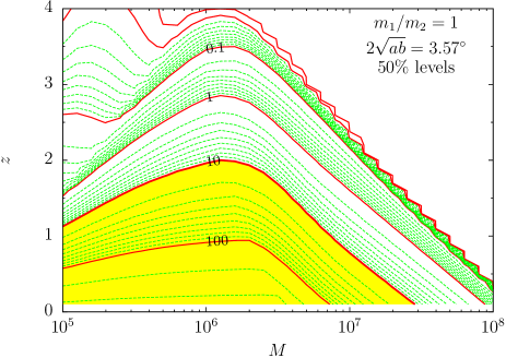
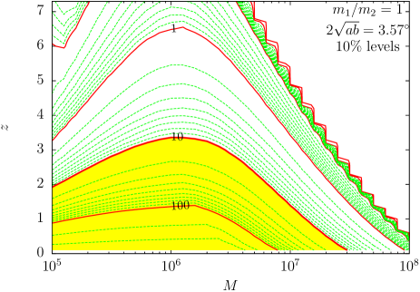
Figure 5: Contours of advance warning times in the total mass ($M$) and redshift ($z$) plane with SMBH mass ratio $m_{1}/m_{2}=1$. The contours trace the look–back times at which the equivalent radius ($2\sqrt{ab}$) of the localization error ellipsoid first reach an LSST-equivalent field-of-view ($3.57^{\circ}$). The contours correspond to the $50\%$ (top) and $10\%$ (bottom) level of cumulative distributions for random orientation events. The contours are logarithmically spaced in days and $10$ days is highlighted with a thick line.

Advance warning time contours are logarithmically spaced, with solid-red contours every decade and a thick red line highlighting the $10\,$day contour. Since advance warning times were computed on a finite mesh, contour levels for arbitrary $M$ and $z$ values were obtained by interpolation. Our interpolated mesh is smooth if $t_{\mathrm{f}}\sim 0.1\,$day, but it gets edgy for short advance warning time approaching ISCO. Figure 5 shows that a $10$ day advance warning is possible with a unique LSST-type pointing for a large range of masses and source redshifts, up to $M\sim 3\times 10^{7}\mathrm{M}_{\odot}$ and $z\sim 1.9$. The bottom shows how far the advance warning concept can be stretched, by focusing on the $10\%$ best cases of random orientation events. In this case a 10 day advance warning is possible up to $z\sim 3$ for masses around $M\sim 10^{6}\mathrm{M}_{\odot}$. Note that, in both cases, allowing for a warning of just one day would extend considerably the range of masses and redshifts for which a unique LSST-type pointing is sufficient.

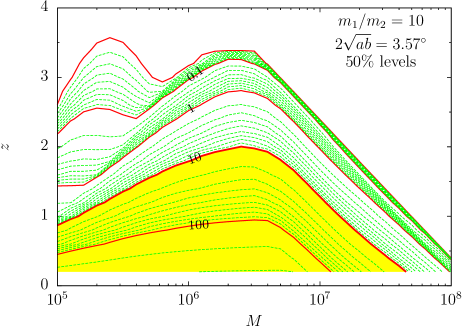
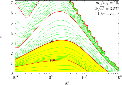
Figure 6: Same as Fig. 5, except for a SMBH mass ratio of $m_{1}/m_{2}=10$.

These results can also be generalized to unequal-mass SMBH binaries. At fixed total mass, $M$, an unequal-mass binary has an instantaneous signal-to-noise ratio that is reduced because of a lower $\eta$ value, but it also has a total observation time that is potentially longer. Localization errors for unequal-mass inspiral events with total observation times longer than a month (i.e. with $\eta_{0.25}^{2/5}(1+z)\,M<1.8\times 10^{7}\mathrm{M}_{\odot}$) are degraded relative to the equal-mass cases discussed so far. For larger total mass, however, the worsening of errors is mitigated, or even reverted, relative to the equal mass case, thanks to the longer observation time. The error ellipsoid also becomes less eccentric thanks to this additional observation time. Figure 6 summarizes results on advance warning times from the same MC computations as in Fig. 5, but this time for unequal-mass SMBH binaries with mass ratio $m_{1}/m_{2}=10$. Despite a systematic degradation in advance warning times (especially noticeable at low $M$ values), the main effect of introducing a mass ratio $m_{1}/m_{2}=10$ is to shift advance warning time contours to somewhat larger values of total mass, $M$. Our main conclusions on advance warning times are not very strongly affected by the inequality of mass components in the population of SMBH binaries considered.

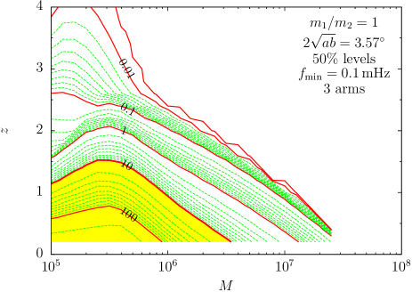
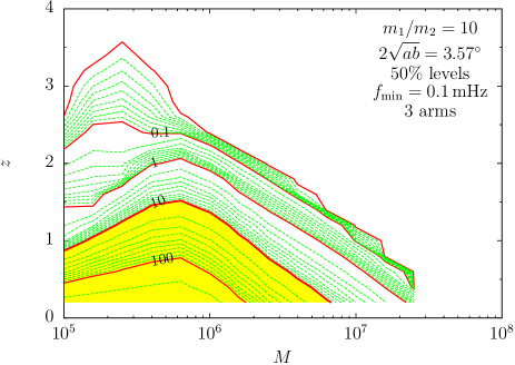
Figure 7: Same as the top panels of Figs. 5 and 6, except for a degraded minimum detector frequency of $f_{\min}=0.1\,\mathrm{mHz}$.

Finally, it is important to understand how sensitive the results are to the LISA detector characteristics. In particular, we examined how advance warning times are affected by increasing the minimum frequency noise wall or by loosing one of the arms of the 3-arm constellation. Figure 7 displays results for $f_{\min}=10^{-4}\,\mathrm{Hz}$, for $m_{1}/m_{2}=1$ and $m_{1}/m_{2}=10$. Increasing $f_{\min}$ mostly reduces the total observation time for high mass inspirals ($t_{\mathrm{i}}\sim f_{\min}^{-8/3}M_{z}^{-5/3}$; see eq. [2]) and reduces the signal-to-noise ratio by a small factor. As a result, the advance warning time contours primarily shift in the $(M,z)$ plane in the direction of smaller total masses by a factor of $\sim 7$, and secondly shift moderately ($30$–$50\%$) to smaller redshifts. Loosing one LISA arm (i.e. using only one of the two interferometers) most importantly removes the ability of the second datastream to break correlations in localization errors and also reduces the signal-to-noise by a small factor. As a result errors do not improve much during the last $\sim 10\,$days before merger. Compared to the case with two interferometers, contours representing an advance warning of less than 10 days are shifted to significantly smaller $z$ (especially for the minor axis of the sky localization ellipsoid), close to the $10$–day contour, but warning times beyond $\sim 10\,$days worsen only moderately. We conclude that even if $f_{\min}=0.1\,\mathrm{mHz}$ or if only one of the two interferometers is used, LISA still admits $10$–day advance localizations for a broad range of masses and redshifts, between $10^{5}\mathrel{\hbox to0.0pt{\lower 4.0pt\hbox{\hskip 1.0pt$\sim$}\hss}\raise 1.0pt\hbox{$<$}}M\mathrel{\hbox to0.0pt{\lower 4.0pt\hbox{\hskip 1.0pt$\sim$}\hss}\raise 1.0pt\hbox{$<$}}2\times 10^{6}$ and $z\mathrel{\hbox to0.0pt{\lower 4.0pt\hbox{\hskip 1.0pt$\sim$}\hss}\raise 1.0pt\hbox{$<$}}1$.

VII Discussion

We have introduced a novel technique, the HMD method, to compute time–dependent GW inspiral signals for LISA. The method relies on the fact that LISA’s orbital motion induces a modulation on timescales that are long relative to the inspiral GW frequency. Since this modulation is periodic, with a fundamental frequency of $f_{\oplus}$, it can be expanded in a discrete Fourier sum. In the HMD formalism, dependencies on sky position, orbital angular momentum orientation, and detector orientation in the LISA signal are inscribed in time-independent coefficients, while time-dependent basis functions are independent of these angles. This decomposition helps to reduce the computational cost of Monte Carlo simulations exploring the time-dependence of source localization errors by orders of magnitude.

Moreover, the HMD method can be used in conjunction with plausible approximations to further decrease the computational cost of explorations of the parameter space of localization errors for LISA inspiral events. In our analysis, we identified two different characteristic frequency constituents of the signal: the high frequency restricted post-Newtonian GW inspiral waveform and the low frequency amplitude modulation resulting from the detector’s orbital motion. In the HMD method, these two components separate and parameters that depend only on the low frequency modulation (such as the source position and the orbital angular momentum angle) can be estimated independently of the other source parameters determined by the high frequency carrier signal. Our working assumption was that cross-correlations among these two sets of parameters must be much smaller than parameter correlations within either set. This hypothesis is valid very generally in the no spin limit for SMBHs, as shown by full Fisher matrix calculations without such approximations for general relativity hug02 and alternative theories of gravity bbw05 .

In order to further examine the validity of our assumptions and the ultimate boundaries of our models, and to understand our results, we have constructed illustrative toy models that we now describe in some detail. These toy models show that the separation of parameters into various subsets associated with different characteristic frequencies of the signal is a rather general property, which turns out to be an efficient way of reducing the computational cost of error estimations for the LISA problem.

VII.1 Simple toy models

In this section, we discuss very simple toy models which capture the essence of the problem posed by the time-evolution of parameter error estimations. We then use these models to answer general questions on the LISA-specific parameter estimation problem.

Our harmonic decomposition technique is based on the simple intuition that the angular information can be deduced from the slow periodic modulation of the high frequency GW waveform. In § III, we have shown that modulation harmonics with frequencies larger than $4f_{\oplus}$ vanish exactly. Here, we discuss the general properties of such a modulation. In the case of LISA, the high frequency carrier signal has an effective, cycle-averaged signal-to-noise ratio which monotonically increases with time as SMBH binaries approach merger. To mimic such events, we also assume in all of our toy models that the instantaneous signal-to-noise ratio continuously improves throughout the observation.

We seek answers to the following questions:

1. How do mean errors evolve during the final days of observation?

   On the one hand, in standard angle-averaged treatments (e.g. bbw05 ; koc06 ; aru06 ), an evolution of errors with the inverse of the signal-to-noise ratio is generally assumed. This would suggest a large improvement during the last day of inspiral. On the other hand, the slow modulation picture suggests just the contrary: not much improvement is expected at late times when there is effectively very little modulation (Finn & Larson 2005, private communication).

2. Does the introduction of additional high frequency components in the signal have any effect on the estimations of low frequency parameters?

   In the GW context, it is of general interest to determine under what circumstances additional high frequency signal components, such as higher order post-Newtonian corrections or spin-induced effects, remain decoupled from the determination of angular and distance information based on the signal amplitude modulation.

3. Are there combinations of signal parameters for which errors improve rapidly in the last days of observation? If so, what are these combinations? What determines how many such rapidly–improving combinations there will be?

   If the distance $d_{\rm L}$ correlates with the angles, then in principle the volume of the 3D error box can be much smaller than the product of the marginalized errors $\delta\Omega\times\delta d_{\rm L}$ would imply. Unfortunately, in practice, this is unlikely to help to reduce the number of false counterparts, because the $\delta z$ error will be dominated by weak lensing koc06 .

4. How does the width of parameter error distributions evolve with time? Are the best and worst cases approaching the typical case prior to the final days of observation? How do we expect the eccentricity of localization error ellipsoid to evolve with time for LISA?

Here, we restrict our discussion to a brief summary of our findings and direct the reader to Appendix A for further details on these toy models.

The parameter estimation uncertainties are defined by the correlation error matrix. For $N_{p}$ parameters, this defines an $N_{p}$-dimensional error-ellipsoid in the $N_{p}$-dimensional parameter space, where parameters are constrained at a given confidence level. Marginalized errors for a given parameter are then related to the projection of this ellipsoid on the basis vector corresponding to that parameter. Since the principal axes of this error ellipsoid are generally not aligned with the original parameters, the marginalized errors can be substantial even if the volume of the error ellipsoid is close to zero. This happens if the ellipsoid is very “thin” but has a large size in at least one direction. Diagonal elements of the correlation matrix provide marginalized squared errors on the parameters, while eigenvalues provide squared errors along the principal axes.

We consider three versions of toy signals to understand how a particular harmonic mode contributes to the time-dependence of parameter uncertainties and to find answers to Questions 1–4 above. We start with the simplest toy model and refine this model by adding more details and complexity in the successive models. In each case, we discuss general implications for the model under consideration.

VII.1.1 Basic toy model

In our basic toy model, we assume that the true signal is comprised of a constant carrier signal, which is modulated by a single known-frequency cosine, $f_{\oplus}$:

$$h(t)=c_{0}+c_{1}\cos(2\pi f_{\oplus}t),$$ (81)

where $c_{0}$ and $c_{1}$ are unknown parameters to be estimated. We assume that the noise level is rapidly decreasing during the observation, mimicking the gradual increase in the instantaneous signal-to-noise ratio for LISA inspiral signals. The contradictory statements made in relation to Question 1 above can be explored with this model. We find that marginalized parameter errors scale with the signal-to-noise ratio far away from merger (i.e. $t_{\mathrm{f}}\mathrel{\hbox to0.0pt{\lower 4.0pt\hbox{\hskip 1.0pt$\sim$}\hss}\raise 1.0pt\hbox{$>$}}0.1f_{\oplus}^{-1}$) but they quickly converge to their final values at late times, even though the signal-to-noise ratio keeps accumulating. It is possible to derive analytical formulae for the evolution of parameter errors to fully characterize this behavior (see Appendix A). We find that, even though the error ellipse rapidly decreases in volume, as the inverse of the signal-to-noise ratio near merger, the error ellipse only shrinks along one of its dimensions, the semi-minor axis, so that a non-negligible residual uncertainty remains in the orthogonal subspace (e.g. along the semi-major axis). This residual uncertainty carries over to final marginalized errors for both parameters. Therefore, this first toy model verifies the second option in relation to Question 1.: there is no late improvement because there is very little effective signal modulation, making the signal-to-noise argument largely irrelevant. However, we find below that this model does not carry some essential features of the LISA signal which modify somewhat our final answer to Question 1 (see final toy model below).

VII.1.2 Second toy model

In our toy second model, we modify the single frequency signal by postulating two pairs of unknown amplitudes and phases for two different a priori known frequencies, satisfying $f_{2}\gg f_{1}$, which modulate an otherwise constant signal:

$$h(t)= c_{0}+s_{1}\sin(2\pi f_{1}t)+c_{1}\cos(2\pi f_{1}t)$$ (82)

$$+ s_{10}\sin(2\pi f_{2}t)+c_{10}\cos(2\pi f_{2}t).$$

The number of unknowns in this model is five: $c_{0},s_{1},c_{1},s_{10}$ and $c_{10}$ are the coefficients of the functions $1$, $\sin(2\pi f_{1}t)$, $\cos(2\pi f_{1}t)$, $\sin(2\pi f_{2}t)$, and $\cos(2\pi f_{2}t)$. Again, we assume that the noise decreases quickly with time before merger, at $t=0$. This model is designed to answer our Question 2 above. In this case, we find that parameter errors are correlated only with unique frequency components and the constant signal, all the way to $t_{\mathrm{f}}\mathrel{\hbox to0.0pt{\lower 4.0pt\hbox{\hskip 1.0pt$\sim$}\hss}\raise 1.0pt\hbox{$>$}}0.1f_{2}^{-1}$. The model thus demonstrates how components associated with very different variation timescales can decouple from each other. Moreover, as for the first toy model, we find that marginalized parameter errors effectively stop improving past a finite time before merger (Question 1), which is simply related to their respective frequencies. As a result, a nonzero residual error remains again, even though the signal-to-noise ratio continuously increases near merger.

VII.1.3 Final toy model

In our final toy model, we insert a few additional features essential to a realistic LISA data-stream. Firstly, we assume 5 low-frequency harmonics, $1$, $\sin(2\pi f_{1}t)$, $\cos(2\pi f_{1}t)$, $\sin(4\pi f_{1}t)$, $(\sin 4\pi f_{1}t)$, with unknown amplitudes. We also include a high frequency carrier signal with known frequency, $f_{2}\gg f_{1}$, but unknown amplitudes in $\sin(2\pi f_{2}t)$ and $\cos(2\pi f_{2}t)$, for a total of seven free parameters. Secondly, we note that the LISA system is equivalent to two orthogonal arm interferometers with both detectors measuring polarization phases simultaneously (which correspond to the real and imaginary parts of the amplitude modulation, § IV). Therefore, the signal is comprised of 4 simultaneous data-streams. We incorporate this feature by assuming 4 measurements (i.e. 4 corresponding Fisher matrices) of the signal with 4 given phase shifts ($\varphi^{s_{1}}_{i},\varphi^{c_{1}}_{i},\varphi^{s_{2}}_{i},\varphi^{c_{2}}_{i}$; $1\leq i\leq 4$) so that

$$h(t) = c_{0}+s_{1}\sin(2\pi f_{1}t+\varphi^{s_{1}}_{i})+c_{1}\cos(2\pi f_{1}t+\varphi^{c_{1}}_{i})$$ (83)

$$+s_{2}\sin(2\pi f_{1}t+\varphi^{s_{2}}_{i})+c_{2}\cos(2\pi f_{1}t+\varphi^{c_{2}}_{i})$$

$$+s_{10}\sin(2\pi f_{2}t)+c_{10}\cos(2\pi f_{2}t),$$

In this case, we find that 4 principal components improve quickly at late times. As in our second toy model, the high frequency parameters decouple from the slow frequency ones, except at very late times when $t_{\mathrm{f}}\mathrel{\hbox to0.0pt{\lower 4.0pt\hbox{\hskip 1.0pt$\sim$}\hss}\raise 1.0pt\hbox{$>$}}0.1f_{2}^{-1}$.

This final toy model allows us to answers all of Questions 1-4 as follows.

• Answer 1: Four out of 5 slow principal components of the error ellipsoid are quickly improving with time, while one of them stops improving at $t_{\mathrm{f}}\mathrel{\hbox to0.0pt{\lower 4.0pt\hbox{\hskip 1.0pt$\sim$}\hss}\raise 1.0pt\hbox{$<$}}0.1f_{1}^{-1}$. Therefore, any parameter with a large projection along this one poor principal component will stop improving, while parameters nearly orthogonal to it will keep improving quickly. Thus, both statements made in relation to Question 1 above can in fact be correct, depending on the connection between a given parameter and the poor principal component. Typically, we expect marginalized parameter uncertainties to evolve as $(S/N)^{-1}$ for $t_{\mathrm{f}}\mathrel{\hbox to0.0pt{\lower 4.0pt\hbox{\hskip 1.0pt$\sim$}\hss}\raise 1.0pt\hbox{$>$}}0.1f_{1}^{-1}$. For smaller $t_{\mathrm{f}}$ values, closer to merger, they would continue to improve, albeit with a shallower slope.

• Answer 2: We find that the introduction of additional high frequency components does not change the evolution of original parameter estimations as long as the time-to-merger is larger than a fraction of the time period of the additional high frequency components.

• Answer 3: As the signal-to-noise ratio increases quickly at late times, rapidly evolving parameter error combinations are given by the principal components of the error ellipsoid corresponding to the final situation at merger. With 4 data-streams, there are 4 such best principal components. Analogously, for the LISA amplitude modulation given by eq. (25), we expect that the 2 polarization phases for the 2 beam patterns at ISCO can be best determined: $(1+\cos^{2}\theta_{NL})F^{I,II}_{+}(\Omega_{\rm ISCO})$ and $\cos\theta_{NL}F^{I,II}_{\times}(\Omega_{\rm ISCO})$. (In terms of ecliptic angular variables, these are the real and imaginary parts of the combination given by eq. (34).)

• Answer 4: The widths of error distributions for slow parameters do not change significantly as long as $t_{\mathrm{f}}\mathrel{\hbox to0.0pt{\lower 4.0pt\hbox{\hskip 1.0pt$\sim$}\hss}\raise 1.0pt\hbox{$>$}}0.1f_{1}^{-1}$. During this final stretch of time before merger, however, one of the principal components stops improving and the major axis of the error ellipsoid freezes. Since the physical parameters can be considered to be randomly oriented with respect to the ellipsoid axes, distributions of marginalized errors suddenly start broadening for $t_{\mathrm{f}}\mathrel{\hbox to0.0pt{\lower 4.0pt\hbox{\hskip 1.0pt$\sim$}\hss}\raise 1.0pt\hbox{$<$}}0.1f_{1}^{-1}$, with a worst case relative orientation leading to very little improvement and a best case relative orientation corresponding to a scaling with $(S/N)^{-1}$.

VII.2 Implications for LISA

These simple toy models offer a general interpretation of the time dependence of LISA’s parameter estimation errors for source localization. The LISA data stream is described by $N_{p1}=5$ physical parameters, ${\bm{p}}_{\mathrm{slow}}$, which are not the harmonic coefficients themselves but determine these coefficients, $g_{j}$ (or conversely, the mode expansion coefficients $g_{j}$ determine the physical parameters ${\bm{p}}_{\mathrm{slow}}$; see § III). Neglecting Doppler phase and spin precession effects, $2J_{\max}+1=9$ modes determine the signal by eqs. (41,42). In principle, any $N_{p1}=5$ of the $g_{j}$ mode amplitudes uniquely determine the physical parameters, ${\bm{p}}_{\mathrm{slow}}$. However, in the presence of noise, each of these modes are uncertain and the combination of all modes helps in reducing the estimation errors of the ${\bm{p}}_{\mathrm{slow}}$ variables.

The key implication of our toy models for LISA is that the estimation of low frequency $g_{j}$ modes with low $|j|$ are effectively decoupled from the high frequency signal, unless the merger is within $\sim 0.1$ times the cycle time of the fast-oscillating signal. We have shown that the HMD of the orbital modulation consists purely of low-order harmonics, with $|j|\leq 4$. In comparison, the high frequency GW phase has a much higher frequency, corresponding to $j>1000$, and this high frequency signal’s cycle time is greater than the time to merger throughout $t\mathrel{\hbox to0.0pt{\lower 4.0pt\hbox{\hskip 1.0pt$\sim$}\hss}\raise 1.0pt\hbox{$>$}}t_{\rm ISCO}$. Hence, physical parameters ${\bm{p}}_{\mathrm{slow}}$ will remain decoupled from parameters ${\bm{p}}_{\mathrm{fast}}$, all the way to ISCO. This finding is independent of details of the waveform and the modulation, in agreement with the results of Ref. bbw05 which show that decoupling occurs independently of the details of the $h_{\mathrm{c}}(t)$ signals, including the modified inspiral waveforms of alternative theories of gravity. In terms of post-Newtonian expansions, only terms above second order have cycle times as large as the cycle time of the amplitude modulation. These terms are responsible for the small cross-correlations of the two sets of parameters found by Ref. hug02 .

We have not considered spin precession effects, but Vecchio vec04 and Lang & Hughes lh06 find that spin precession effects can help improve the final localization errors by a factor of $\sim 3$. Spin precession cycle times decrease continuously, become of order a few days or less during the last week prior to merger, and of order hours during the last day of inspiral. Therefore, according to our simple models, we expect spin precession effects to improve the source parameter estimation errors especially during the final two weeks before ISCO. During that period of time, in the absence of spin effects, parameter uncertainties (especially the sky position major axis and the luminosity distance) cease to improve when using only the amplitude modulation.

The best-determined parameters at ISCO are, approximately, the independent detector outputs at ISCO, i.e. the real and imaginary parts of $h^{\rm I,II}_{1}(p_{1})$: $d_{\rm L}^{-1}(1+\cos^{2}\theta_{NL})F^{I,II}_{+}(\Omega)$ and $d_{\rm L}^{-1}\cos\theta_{NL}F^{I,II}_{\times}(\Omega)$ (see Appendix A.4). These are the 4 independent combinations of 5 physical parameters $p_{1}$ which correspond to the eigenvectors of the error covariance matrix following the steep evolution $\propto(S/N)^{-1}$ all the way to ISCO. We refer to the fifth independent combination, which is orthogonal to these best eigenvectors, the “worst” eigenvector, since for this combination, the evolution ceases to improve as $(S/N)^{-1}$ within $\sim 0.1\times(\rm amplitude~{}modulation~{}cycle~{}time)$ of merger. It is straightforward to obtain this worst combination explicitly by using the 4 other eigenvectors and Gram-Schmidt orthogonalization (but we have not done this in practice). Since the highest frequency harmonic of the slow modulation is for $j=4$, the corresponding cycle time is $\,\mathrm{yr}/4$. Thus, we expect errors will stop improving roughly $1$–$2$ weeks prior to merger. Distributions of errors will quickly broaden during these final stages of observation before ISCO. Simply scaling errors with $(S/N)^{-1}$, as in the angle-averaged formalism (e.g. bbw05 ; koc06 ), is acceptable if one studies the evolution of parameter errors at $t_{\mathrm{f}}\mathrel{\hbox to0.0pt{\lower 4.0pt\hbox{\hskip 1.0pt$\sim$}\hss}\raise 1.0pt\hbox{$>$}}2$ weeks, or if one only focuses on the best case parameter combinations. In general, the exponent in the $(S/N)$ scaling decreases as one approaches merger time depending on how close the particular combination of angles considered is to the worst combination.

Our findings for the eccentricity evolution of LISA’s sky localization error ellipsoid can also be understood with the simple toy models. In fact, we found this behavior to be expected for any model signal with relative instantaneous signal amplitude increasing quickly with time, e.g. $t^{-\alpha}$, $\alpha\mathrel{\hbox to0.0pt{\lower 4.0pt\hbox{\hskip 1.0pt$\sim$}\hss}\raise 1.0pt\hbox{$>$}}2$. In this case, the principal axes of the general parameter error ellipsoid separate near $t_{\mathrm{f}}=0$. There are a limited number of principal errors which rapidly decrease to zero near $t_{\mathrm{f}}=0$, while others “freeze out” at a time related to a fraction of the cycle time of the particular waveform ($\sim 0.1T_{\rm cycle}$ if $t_{\mathrm{i}}>T_{\rm cycle}$). For LISA, there are 5 variable parameters, ${\bm{p}}_{\mathrm{slow}}=(d_{\rm L},\theta_{N},\phi_{N},\theta_{L},\phi_{L})$, and estimation uncertainties of 4 combinations of these parameters, $d_{\rm L}^{-1}(1+\cos^{2}\theta_{NL})F^{I,II}_{+}(\Omega),d_{\rm L}^{-1}\cos\theta_{NL}F^{I,II}_{\times}(\Omega)$, improve quickly with $(S/N)^{-1}$. These combinations correspond to the best 4 principal axes of the 5-dimensional error ellipsoid. The remaining $5^{\rm th}$ principal axis does not improve as $(S/N)^{-1}$, but rather stops improving at a fraction of the last modulation cycle time. The two dimensional sky position error ellipsoid is the projection of the general 5-dimensional error ellipsoid on the $(\theta_{N},\phi_{N})$ plane. This plane will generally not be aligned with the principal axes of the 5-dimensional ellipsoid. In a typical case, therefore, there will be a nonzero projection on the worst principal component and the sky position ellipsoid will stop shrinking along the worst principal component. This explains why the major axis, $2a$, ceases to improve and the eccentricity increases close to merger.

According to this argument, it is somewhat surprising to find that the minor axis, $2b$, can stop improving much before ISCO. Figure 2 shows that this happens in the worst $10\%$ of all cases for randomly chosen source angular parameters. The reason for this is that, in some cases, not all rapidly improving “best” principal components have a small absolute error at ISCO. For example, consider an edge-on binary inspiral ($\cos\theta_{NL}\approx 0$). Since two of the quickly improving parameters are simply proportional to $\cos\theta_{NL}$, the errors will be very large for these parameters. Thus, depending on the relative orientation of the detector and the source at ISCO, there can be large absolute errors in some cases even for the best combinations of parameters. In short, both axes of the sky position error ellipsoid can stop improving at late times in those cases when LISA is oriented in its least favorable direction at ISCO.

VIII Conclusions

We have developed a new harmonic mode decomposition (HMD) method to study the feasibility of using LISA inspiral signals to locate coalescing SMBH binaries in the sky, as the mergers proceed. According to our extensive HMD survey of potential LISA sources, it will be possible to trigger large field-of-view searches for prompt electromagnetic counterparts during the final stages of inspiral and coalescence. Our results indicate, for instance, that for a typical $z\sim 1$ merger event with total mass $M\sim 10^{5}-10^{7}\mathrm{M}_{\odot}$, a 10-day advance notice will be available to localize the source to within a $10\deg^{2}$ region of the sky. The advance notice to localize the source to a 10 times smaller area of $1\deg^{2}$ is $<1$ day for the typical event, suggesting that a wide–field instrument of the LSST class, with a $10\deg^{2}$ field-of-view, may offer significant advantages over a smaller, $1\deg^{2}$ field-of-view instrument for observational efforts to catch prompt electromagnetic counterparts to SMBH binary inspirals.

The robust identification of such electromagnetic counterparts would have multiple applications, from an alternative method to measure cosmological parameters to precise measurements of merger geometries in relation to host galaxy properties hh05 ; koc06 . If such electromagnetic counterpart searches can be implemented effectively and successfully, LISA could become an extremely valuable instrument for astrophysics and cosmology, beyond the original general relativistic measurement goals. Given the advance warning time capabilities established here, effective strategies for electromagnetic counterpart searches, including the concept of partially dedicating a $\mathrel{\hbox to0.0pt{\lower 4.0pt\hbox{\hskip 1.0pt$\sim$}\hss}\raise 1.0pt\hbox{$>$}}10\deg^{2}$ field-of-view fast survey instrument of the LSST class, are considered in detail in a separate investigation paper2 .

Appendix A Simple Toy Models

A.1 Single Frequency Model

First, let us consider the following simple model with two unknowns, $c_{0}$ and $c_{1}$,

$$h(t)=c_{0}+c_{1}\cos(2\pi f_{\oplus}t),$$ (84)

where $f_{\oplus}\equiv\,\mathrm{yr}^{-1}$ is fixed and assumed to be known prior to the observation. We call $t$ the “look–back time” before merger. Let us assume that the relative noise continuously decreases during the observation and that the differential squared signal-to-noise ratio (without modulation) is given by $\sigma^{-2}(t)=t^{-2}$ in eq. (50). Here $t=0$ is a proxy for the “merger”. Close to merger, the signal-to-noise ratio accumulates very rapidly. We assume that $h(t)$ is measured in the time interval $t_{\mathrm{i}}\geq t\geq t_{\mathrm{f}}$, where $t_{\mathrm{i}}$ is the start of observation, $t_{\mathrm{f}}$ is the end of observation (i.e. $x=t_{\rm merger}-t$, $x_{\min}=t_{\mathrm{f}}$, and $x_{\max}=t_{\mathrm{i}}$ in eq. [50]). We fix $t_{\mathrm{i}}$ and examine the dependence of parameter estimation errors as a function of $t_{\mathrm{f}}$, assuming $t_{\mathrm{f}}\ll t_{\mathrm{i}}$.

Note that, for the signal (84), the fiducial values $(c_{0},c_{1})$ drop out when calculating the RMS parameter errors $\Delta c_{0}$ and $\Delta c_{1}$ using eq. (50). More generally, this is true for any signal which is a linear combination of the unknown parameters. All our toy models will have this property and the results presented in this section will be general in that respect.

First, let us substitute (84) in (49) and (50), and evaluate the expected covariance matrix numerically. Figure 8 displays the time dependence of marginalized parameter errors and principal errors. The plots show that the parameter errors all decrease with the signal to noise ratio when the look–back time before merger is large. However if the end of the observation is within a certain critical time to merger, $t_{\mathrm{f}}<t_{\mathrm{c}}$, only one principal component follows the signal-to-noise ratio. Figure 8 shows that $t_{\mathrm{c}}\sim 0.1\,\mathrm{yr}$. The start of the observation in Figure 8 was fixed at $t_{\mathrm{i}}=5\,\mathrm{yr}$.

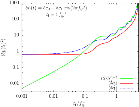
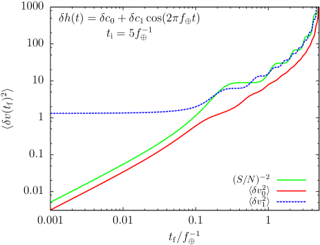
Figure 8: Marginalized parameter errors (top) and principal errors (bottom) for the single frequency model. The green curve shows the scaling with inverse squared signal-to-noise ratio, $(S/N)^{-2}$, for reference on both plots. A total observation of $t_{\mathrm{i}}=5\,\mathrm{yr}$ is assumed. Marginalized errors follow the signal-to-noise ratio for large $t_{\mathrm{f}}$, but they stop improving within $t_{\mathrm{f}}<t_{\mathrm{c}}\sim 0.1\,\mathrm{yr}$ from merger. Only one eigenvalue scales with the signal-to-noise ratio near merger.

It is also interesting to examine what happens for general total observation times, do errors stop improving within some time $t_{\mathrm{c}}$ before merger? If yes, how does $t_{\mathrm{c}}$ depend on the two timescales $t_{\mathrm{i}}$ and $f_{\oplus}^{-1}$? We examine this question numerically, substituting (84) in (49) and (50) and now varying both $t_{\mathrm{f}}/f_{\oplus}^{-1}$ and $t_{\mathrm{i}}/f_{\oplus}^{-1}$. Let us define the critical end-of-observation, $t_{\mathrm{c}}$, as the time when the marginalized squared parameter error is first within a factor of 2 of its final value. Figure 9 plots the result for the two parameters. Figure 9 shows that $t_{\mathrm{c}}$ is determined by $f_{\oplus}^{-1}$ for large $t_{\mathrm{i}}$, but becomes $t_{\mathrm{i}}$-dependent for lower $t_{\mathrm{i}}$ values. In the limit $t_{\mathrm{i}}\ll f_{\oplus}^{-1}$, the critical look–back time is independent of $f_{\oplus}^{-1}$, it becomes a constant fraction of $t_{\mathrm{i}}$.

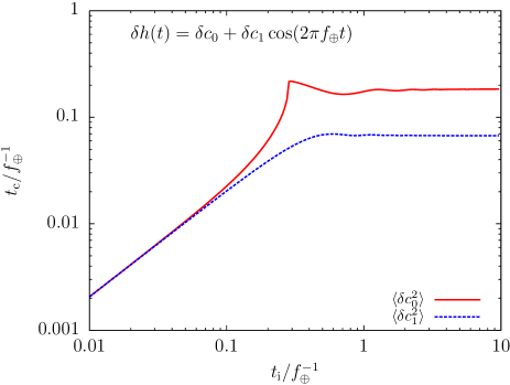
Figure 9: Critical look–back time, $t_{\mathrm{c}}$, at which parameter errors stop improving. Here $t_{\mathrm{c}}$ is defined as the time at which marginalized squared errors are within a factor of 2 of their final values for the first time.

Note that, in the limit of an observation extending up to merger, at $t=0$, the signal becomes $h(0)=c_{0}+c_{1}$ and it has infinite instantaneous signal-to-noise ratio. Therefore, this is the best combination of parameters for which the scaling of errors can follow $(S/N)^{-1}$ all the way to $t=0$. The worst combination is $c_{0}-c_{1}$, which stops improving before $t=0$.

For this simple model, the origin of these features can be understood by analyzing the principal errors and the marginalized errors in the error covariance matrix. For this purpose, we present an analytical algebraic solution to this problem. To simplify the equations, let us set the time-scale to $f_{\oplus}^{-1}/(2\pi)$. In this case the Fisher matrix (50) is

$$\Gamma_{ij}(t_{\mathrm{f}},t_{\mathrm{i}})=\left(\begin{array}[]{cc}\int_{t_{\mathrm{f}}}^{t_{\mathrm{i}}}t^{-2}\mathrm{d}t&\int_{t_{\mathrm{f}}}^{t_{\mathrm{i}}}\cos(t)t^{-2}\mathrm{d}t\\ \int_{t_{\mathrm{f}}}^{t_{\mathrm{i}}}\cos(t)t^{-2}\mathrm{d}t&\int_{t_{\mathrm{f}}}^{t_{\mathrm{i}}}\cos^{2}(t)t^{-2}\mathrm{d}t\\ \end{array}\right).$$ (85)

The integrals can be evaluated analytically,

$$\Gamma_{ij}(t_{\mathrm{f}},t_{\mathrm{i}})=\left.\left(\begin{array}[]{cc}\frac{1}{t}&\frac{\cos(t)}{t}+\mathrm{Si}(t)\\ \frac{\cos(t)}{t}+\mathrm{Si}(t)&\frac{\cos(2t)+1}{2t}+\mathrm{Si}(2t)\\ \end{array}\right)\right]^{t_{\mathrm{f}}}_{t_{\mathrm{i}}},$$ (86)

where $\mathrm{Si}(x)=\int_{0}^{x}\frac{\sin(x)}{x}\mathrm{d}x$ is the sine integral.

In the next two subsections, we find the limiting behavior of marginalized and principal parameter errors in two different limits: $f_{\oplus}^{-1}\ll t_{\mathrm{i}}$ and $t_{\mathrm{i}}\ll f_{\oplus}^{-1}$, respectively.

A.1.1 Long Observations $(f_{\oplus}^{-1}\ll t_{\mathrm{i}})$

Here, we assume that the signal has been measured for a very long total time and we concentrate on the effects of changing the end of the observation time, $t_{\mathrm{f}}$, near merger. Therefore, we take the limit $t_{\mathrm{i}}\rightarrow\infty$, for which

$$\Gamma_{ij}(t_{\mathrm{f}}) = \left(\begin{array}[]{cc}\frac{1}{t_{\mathrm{f}}}&\frac{\cos(t_{\mathrm{f}})}{t_{\mathrm{f}}}+\mathrm{Si}(t_{\mathrm{f}})\\ \frac{\cos(t_{\mathrm{f}})}{t_{\mathrm{f}}}+\mathrm{Si}(t_{\mathrm{f}})&\frac{\cos(2t_{\mathrm{f}})+1}{2t_{\mathrm{f}}}+\mathrm{Si}(2t_{\mathrm{f}})\\ \end{array}\right)$$ (92)

$$-\left(\begin{array}[]{cc}0&\pi/2\\ \pi/2&\pi/2\\ \end{array}\right).$$

We consider the case of a total observation time which is not negligible compared to a cycle time, $f_{\oplus}^{-1}$, i.e. $t_{\mathrm{f}}\ll t_{\mathrm{i}}$. We next examine two possible cases, $f_{\oplus}^{-1}\ll t_{\mathrm{f}}\ll t_{\mathrm{i}}$ and $t_{\mathrm{f}}\ll f_{\oplus}^{-1}\ll t_{\mathrm{i}}$, separately.

First let us assume that the merger is still far away in time in units of a cycle period $(f_{\oplus}\ll t_{\mathrm{f}}\ll t_{\mathrm{i}})$. We substitute (92) in (49) and expand $\Gamma^{-1}(t_{\mathrm{f}})$ into a $t_{\mathrm{f}}^{-1}$ series:

$$(\Gamma^{-1})_{ij}\approx\frac{t_{\mathrm{f}}}{1-\frac{\sin(2t_{\mathrm{f}})}{2t_{\mathrm{f}}}+\frac{\cos(2t_{\mathrm{f}})-1}{t_{\mathrm{f}}^{2}}}\left(\begin{array}[]{cc}1-\frac{\sin(2t_{\mathrm{f}})}{2t_{\mathrm{f}}}&\frac{2\sin(t_{\mathrm{f}})}{t_{\mathrm{f}}}\\ \frac{2\sin(t_{\mathrm{f}})}{t_{\mathrm{f}}}&2\\ \end{array}\right).$$ (93)

Equation (93) gives the large $t_{\mathrm{f}}$ behavior of marginalized errors and correlations, which can be compared to Figure 8 in the appropriate regime, $t_{\mathrm{f}}>1\,\mathrm{yr}$. In this case, to leading order, all of the squared errors scale with $t_{\mathrm{f}}$, which is the scaling of the inverse squared signal-to-noise ratio, $(S/N)^{-2}$, for our noise model.

Next, let us examine the case when the end-of-observation time is close to merger, i.e. $t_{\mathrm{f}}\ll f_{\oplus}\ll t_{\mathrm{i}}$. Now, taking the inverse of the matrix and expanding into a $t_{\mathrm{f}}$ series around $t_{\mathrm{f}}=0$ gives

$$(\Gamma^{-1})_{ij}\approx\frac{2}{\pi}\left(\begin{array}[]{cc}1+\frac{2}{3\pi}t_{\mathrm{f}}^{3}&-1+\frac{t_{\mathrm{f}}^{2}}{2\pi^{2}}\\ -1+\frac{t_{\mathrm{f}}^{2}}{2\pi^{2}}&1+\frac{\pi}{2}t_{\mathrm{f}}\\ \end{array}\right),$$ (94)

which gives the short timescale behavior of marginalized errors and correlations. The eigenvalues of $\Gamma^{-1}$ define the squared length of the individual principal axes of the parameter error ellipsoid, in this case

$$\left(\begin{array}[]{c}\langle\delta v^{2}_{0}\rangle\\ \langle\delta v^{2}_{1}\rangle\\ \end{array}\right)\approx\left(\begin{array}[]{c}\frac{t_{\mathrm{f}}}{2}+\frac{3\pi}{16}t_{\mathrm{f}}^{2}\\ \frac{4}{\pi}+\frac{t_{\mathrm{f}}}{2}+\left(\frac{5\pi}{16}-\frac{2}{\pi}\right)t_{\mathrm{f}}^{2}\\ \end{array}\right).$$ (95)

Note that, in eqs. (85)-(95), time is measured in units of $f_{\oplus}^{-1}/(2\pi)$. In full units, the squared marginalized parameter errors (i.e. diagonal elements) of (94) become

$$\left(\begin{array}[]{c}\langle\delta c^{2}_{0}\rangle\\ \langle\delta c^{2}_{1}\rangle\\ \end{array}\right)=\left(\begin{array}[]{c}\frac{2}{\pi}\left[1+\left(\frac{t_{\mathrm{f}}}{\sqrt[3]{3/(16\pi^{2})}f_{\oplus}^{-1}}\right)^{3}\right]\\ \frac{2}{\pi}\left[1+\frac{t_{\mathrm{f}}}{\frac{1}{\pi^{2}}f_{\oplus}^{-1}}\right]\\ \end{array}\right).$$ (96)

For the eigenvalues (95), we get

$$\left(\begin{array}[]{c}\langle\delta v^{2}_{0}\rangle\\ \langle\delta v^{2}_{1}\rangle\\ \end{array}\right)=\left(\begin{array}[]{c}t_{\mathrm{f}}/\left({\frac{1}{\pi}f_{\oplus}^{-1}}\right)\\ \frac{4}{\pi}\left[1+\frac{t_{\mathrm{f}}}{\frac{4}{\pi^{2}}f_{\oplus}^{-1}}\right]\\ \end{array}\right).$$ (97)

Equation (96) implies that the evolution of the marginalized squared error on $c_{0}$ is very flat for small $t_{\mathrm{f}}$, when the second term is negligible, i.e. $t_{\mathrm{f}}\ll\sqrt[3]{\frac{3}{16\pi^{2}}}f_{\oplus}^{-1}=0.267\,\mathrm{yr}$, then rises steeply ($\propto t_{\mathrm{f}}^{3}$). The marginalized squared $c_{1}$ error is also constant near merger, for $t_{\mathrm{f}}\ll\frac{1}{\pi^{2}}f_{\oplus}^{-1}\approx 0.1\,\mathrm{yr}$, and it increases $\propto t_{\mathrm{f}}\mathrel{\hbox to0.0pt{\lower 4.0pt\hbox{\hskip 1.0pt$\sim$}\hss}\raise 1.0pt\hbox{$\propto$}}(S/N)^{-2}$ for larger $t_{\mathrm{f}}$. Equation (97) shows that one of the principal errors has a very different time-evolution: it has no constant term proportional to $t_{\mathrm{f}}^{0}$. Therefore the semi-minor axis of the error ellipsoid can decrease continuously with the signal to noise ratio. On the other hand, the semi-major axis becomes constant for $t_{\mathrm{f}}\ll\frac{4}{\pi^{2}}f_{\oplus}^{-1}=0.4\,\mathrm{yr}$. Since the marginalized errors are nontrivial linear combinations of the principal errors, the constant principal error carries over to both marginalized errors and dominates their evolution. All of these findings are in excellent agreement with the numerical results shown in Fig. 8 for $t_{\mathrm{f}}\ll 1\,\mathrm{yr}$ and in Fig. 10 for $t_{\mathrm{i}}/f_{\oplus}^{-1}>1$.

It is worth emphasizing that, even if the total observation time had been infinite, $t_{\mathrm{i}}\to\infty$, the parameters could not have been estimated to infinite precision in this model. It is not very surprising if one recalls that in this model we defined errors to be infinitely large at infinitely early times ($\sigma^{2}(t)\propto t^{2}$). For stationary noise, the contribution of the last cycle to the resultant RMS estimation error for a total observation of $N_{\rm cyc}$ cycles is $1/\sqrt{N_{\rm cyc}}$. In contrast, rather than the total number of cycles, the typical error during the last cycle dominates the determination of noise, for the particular noise model used here.

The main conclusion from this toy model analysis is that errors stop improving close to merger, at $t_{\mathrm{c}}\sim 0.1f_{\oplus}^{-1}$. It can be extended to more general noise models, with $\sigma^{-2}(t)=t^{-\alpha}$ and $\alpha\neq 2$. Repeating the calculations for larger $\alpha$ values, we find that parameter estimation errors become more and more insensitive to very early times, $t_{\mathrm{f}}\ll t\sim t_{\mathrm{i}}$, and that marginalized parameter estimation errors cease to improve at some $t_{\mathrm{c}}$, which is now an $\alpha$-dependent fraction of a single cycle time before merger. For $\alpha>2$, we find that errors increase more abruptly at $t_{\mathrm{f}}\mathrel{\hbox to0.0pt{\lower 4.0pt\hbox{\hskip 1.0pt$\sim$}\hss}\raise 1.0pt\hbox{$>$}}t_{\mathrm{c}}$, which is consistent with the signal-to-noise ratio being a steeper function of time. On the other hand, for lower $\alpha$ values, parameter estimation errors become more and more sensitive to very early times, $t_{\mathrm{f}}\ll t\sim t_{\mathrm{i}}$. In this case, the marginalized parameter estimation errors are again very slowly changing for $0\sim t_{\mathrm{f}}<t_{\mathrm{c}}$, but the approximate time $t_{\mathrm{c}}$ at which parameter errors stop decreasing will be primarily determined by $t_{\mathrm{i}}$, rather than by the cycle period $f_{\oplus}^{-1}$. The transition at $t_{\mathrm{f}}\mathrel{\hbox to0.0pt{\lower 4.0pt\hbox{\hskip 1.0pt$\sim$}\hss}\raise 1.0pt\hbox{$>$}}t_{\mathrm{c}}$ is not as abrupt, but extends to several cycles. The $\alpha=0$ case corresponds to a stationary instantaneous signal-to-noise ratio, with errors scaling slowly as $1/\sqrt{t_{\mathrm{i}}-t_{\mathrm{f}}}$. This case is irrelevant to LISA inspiral signals, which have $\alpha\sim 2$ to a good approximation for $1$day $<t<t_{\mathrm{i}}$ in the relevant range of SMBH masses.

A.1.2 Short observations $(t_{\mathrm{i}}\ll f_{\oplus}^{-1})$

Let us now examine the opposite limiting case, where the start of observation time is already within the final cycle before merger. This is relevant to LISA signals, since the observation time of SMBH inspirals is often below a full year, especially for $(1+z)\,M\geq 4\times 10^{6}\mathrm{M}_{\odot}$.

We again restrict ourselves to the case with a total observation time that is non-negligible, i.e. $t_{\mathrm{f}}\ll t_{\mathrm{i}}$. Using time units of $f_{\oplus}^{-1}/(2\pi)$, expanding (86) into a series of both $t_{\mathrm{i}}$ and $t_{\mathrm{f}}/t_{\mathrm{i}}$, we get

$$(\Gamma^{-1})_{ij} \approx \frac{120}{t_{\mathrm{i}}^{3}(10-t_{\mathrm{i}}^{2})}\left[\left(\begin{array}[]{cc}1&-1\\ -1&1\\ \end{array}\right)\right.$$ (103)

$$\left.+\frac{t_{\mathrm{f}}}{t_{\mathrm{i}}}\left(\begin{array}[]{cc}\frac{30-10t_{\mathrm{i}}^{2}}{10-t_{\mathrm{i}}^{2}}&-\frac{30-5t_{\mathrm{i}}^{2}}{10-t_{\mathrm{i}}^{2}}\\ -\frac{30-5t_{\mathrm{i}}^{2}}{10-t_{\mathrm{i}}^{2}}&\frac{30-\frac{5}{3}t_{\mathrm{i}}^{2}}{10-t_{\mathrm{i}}^{2}}\\ \end{array}\right)\right]$$

Equation (103) gives the parameter estimation covariance during the final stages of observation before merger for small total observation times. In this case, the final errors strongly depend on the total observation time. The errors reach their final values when the second term becomes negligible in eq. (103). To leading order, this happens at $t_{\mathrm{c}}\sim t_{\mathrm{i}}/3$ for both parameters, independently of the cycle time, $f_{\oplus}^{-1}$. Equation (103) approximates well the $t_{\mathrm{i}}$ dependence of $t_{\mathrm{c}}$ shown in Fig. 9 for $t_{\mathrm{i}}/f_{\oplus}^{-1}<0.2$

A.2 Double Frequency Model

Now consider a more elaborate model with five unknowns $c_{0}$, $s_{1}$, $c_{1}$, $s_{10}$, and $c_{10}$:

$$h(t) = c_{0}+s_{1}\sin(2\pi f_{1}t)+c_{1}\cos(2\pi f_{1}t)$$ (104)

$$+s_{10}\sin(2\pi f_{2}t)+c_{10}\cos(2\pi f_{2}t).$$

Here, the signal is comprised of two different characteristic frequencies, $f_{1}$ and $f_{2}$, for which we assume $f_{1}\ll f_{2}$. Moreover we assume that $f_{1}$ and $f_{2}$ are fixed and known prior to the measurement, e.g. we take $f_{1}\equiv 1\,\mathrm{yr}^{-1}$ and $f_{2}\equiv 10\,\mathrm{yr}^{-1}$. We again assume an observation in the look–back time interval $t_{\mathrm{i}}\geq t\geq t_{\mathrm{f}}$ and take the average instantaneous signal-to-noise ratio to increase as $\sigma(t)^{-2}=t^{-2}$.

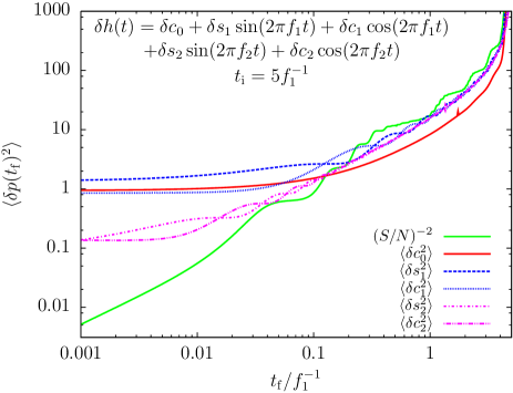
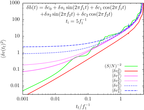
Figure 10: Marginalized parameter errors (top) and principal errors (bottom) for the double frequency model. The green curve shows the scaling with $(S/N)^{-2}$ for reference on both plots. A total observation time $t_{\mathrm{i}}=5\,\mathrm{yr}$ is assumed. Marginalized errors follow the signal-to-noise ratio for large $t_{\mathrm{f}}$ values, but they stop improving after $t_{\mathrm{f}}\mathrel{\hbox to0.0pt{\lower 4.0pt\hbox{\hskip 1.0pt$\sim$}\hss}\raise 1.0pt\hbox{$<$}}0.1f$, for both frequencies. By comparing the two plots, it is clear that high frequency component errors decouple and that they are determined by two corresponding eigenvalues in the bottom panel.

Let us substitute in (49) and (50), and evaluate the expected covariance matrix numerically. Figure 10 displays the results. As in the previous model, these plots show that all parameter errors decrease with signal to noise ratio until the last cycle and all marginalized errors stop improving beyond some nonzero residual error at late times. Thus, the general trends shown in Fig. 10 are very much similar to the ones in the previous simple model (Fig. 8). Again, contrary to the standard $1/\sqrt{N_{\rm cyc}}$ expectation, the error during the last cycle dominates the total error of the accumulated signal. Moreover, comparing Figs. 8 and 10 shows that the presence of additional independent high frequency degrees of freedom practically does not modify the evolution of marginalized parameter errors associated with low frequency components, if $t_{\mathrm{i}}>f_{1}^{-1}$. During the final cycle, the error ellipsoid becomes “thin” and the narrow dimension will not be aligned with any of the parameters. As a result, this bad principal error dominates each of the marginalized parameter errors at late times. (Note that the start-of-observation time in Figure 10 is $t_{\mathrm{i}}=5\,\mathrm{yr}$.)

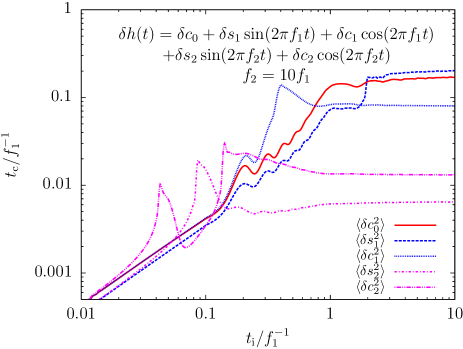
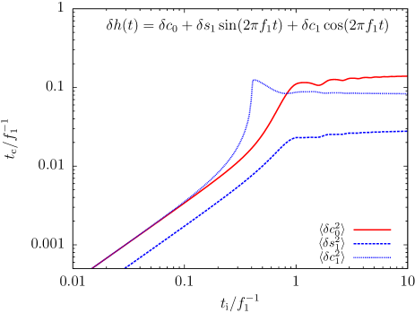
Figure 11: Critical look–back time, $t_{\mathrm{c}}$ (as in Fig. 9), at which marginalized parameter errors stop improving. Top: Only $(c_{0},s_{1},c_{1})$ are allowed to vary, using the prior $(s_{10},c_{10})\equiv(0,0)$. Bottom: All 5 parameters $(c_{0},s_{1},c_{1},s_{10},c_{10})$ are determined from the observation. For $t_{\mathrm{i}}\mathrel{\hbox to0.0pt{\lower 4.0pt\hbox{\hskip 1.0pt$\sim$}\hss}\raise 1.0pt\hbox{$>$}}f_{1}^{-1}$, estimations of low frequency parameters $(c_{0},s_{1},c_{1})$ stop improving at $t_{\mathrm{c}}\sim 0.1f_{1}^{-1}$, while improvement for high frequency parameters occurs all the way to $t_{\mathrm{c}}\sim 0.1f_{2}^{-1}$.

The critical look–back time, $t_{\mathrm{c}}$, at which this happens is different for the different frequency components. The top panel in Fig. 10 shows that ${t_{\mathrm{c}}}_{i}\sim 0.1f_{i}$ approximately for both sets of components $(s_{1},c_{1})$ and $(s_{10},c_{10})$, where $f_{i}$ denotes the corresponding frequencies $f_{1}=1\,\mathrm{yr}^{-1}$ and $f_{2}=10\,\mathrm{yr}^{-1}$, respectively. The bottom panel in Fig. 10 shows that the principal errors separate in three groups. There is one best eigenvector that improves continuously until the end, two that stop improving near ${t_{\mathrm{c}}}_{1}\sim 0.1f_{1}$ and two that stop improving at ${t_{\mathrm{c}}}_{2}\sim 0.1f_{2}$. The high frequency parameters $(s_{10},c_{10})$ totally decouple from the two worst principal components, $(v_{0},v_{1})$, and, as a result, decouple from the low frequency parameters $(c_{0},s_{1},c_{1})$ which are primarily determined by $(v_{0},v_{1})$.

As for our previous model in § A.1, the critical look–back time is generally different for different $t_{\mathrm{i}}$ values. The bottom panel in Figure 11 shows the time $t_{\mathrm{c}}$ at which the squared errors first double, as a function of $t_{\mathrm{i}}/f_{1}^{-1}$, as in Fig. 9. Fig. 11 justifies the rule-of-thumb scaling ${t_{\mathrm{c}}}_{i}\sim 0.1f_{i}$ if the observation time is at least one cycle period, $f_{1}^{-1}$.

The central question for the present analysis is how sensitive is the time evolution of low frequency modulation errors to the presence of high frequency components. We can examine this question by computing the critical look–back time, $t_{\mathrm{c}}$, when the high frequency terms are totally neglected. The top panel in Fig. 9 shows that, if one limits the parameters to $(c_{0},s_{1},c_{1})$, and the total observation time is not smaller than the long-period cycle time, $\sim f_{1}^{-1}$, the resulting $t_{\mathrm{c}}$ value for parameters $c_{0}$ and $c_{1}$ is unchanged at the few percent level. However, if the high frequency components are introduced, the $s_{1}$ error evolves differently since it asymptotes already at much larger $t_{\mathrm{c}}$ values ($\sim 0.1f_{1}^{-1}$ rather than $\sim 0.03f_{-1}$). The reason is that, for small $t$, with a noise level decreasing quickly, the corresponding function $s_{1}\sin(2\pi f_{1}t)\approx 2\pi f_{1}s_{1}t$ is linearly independent of, and thus uncorrelated with, the functions $c_{0}$ and $c_{1}\cos(2\pi f_{1}t)$ which are both constant to first order. Hence, if there are no more unknowns than $(c_{0},s_{1},c_{1})$, then $c_{0}$ and $c_{1}$ are correlated while $s_{1}$ is decoupled and can be determined independently of the other parameters. However, if we add any parameters which are not constant for $t\ll f_{1}^{-1}$, then $s_{1}$ becomes correlated with those. This is exactly what happens in the bottom panel of Fig. 9, when considering the high frequency modulations: the estimation on $s_{1}$ becomes limited for $t\mathrel{\hbox to0.0pt{\lower 4.0pt\hbox{\hskip 1.0pt$\sim$}\hss}\raise 1.0pt\hbox{$<$}}{t_{\mathrm{c}}}_{1}\sim 0.1f_{1}^{-1}$ due to the correlations with $s_{10}$ and $c_{10}$. Quite similarly, if one introduces any other low-frequency function that is not constant to first order, like $s_{2}\sin(4\pi f_{1}t)$, then the correlations with this parameter will limit the improvement of estimation errors for $s_{1}$ at $t_{\mathrm{c}}\sim 0.1f_{1}$, even when neglecting the high frequency components. As we shall see, this is the case for LISA: there are generally more than one $\sin$ and $\cos$ low-frequency modes. In this case, the evolution of estimation errors for low frequency parameters can be obtained with the high frequency modes (like $s_{10}$ and $c_{10}$) priored out. This justifies our simple intuition: once the signal is decomposed into different time-scale components, the parameter estimation problem becomes separable and the evolution of parameter errors corresponding to different such time-scales can be estimated independently from each other.

Rather than going through an analytical derivation as in § A.1, we answer one remaining question here: what combination of the original parameters $(c_{0},s_{1},c_{1},s_{10},c_{10})$ corresponds to the best principal component, $v_{0}$, which can be determined extremely accurately at late times, $t_{\mathrm{f}}\to 0$? At $t=0$, the noise drops to zero. Therefore, the quantity we can measure using the $t=0$ information is simply $h(t=0)$. Looking back at eq. (104), this is $c_{0}+c_{1}+c_{2}$. It will be interesting to look for similar “best determined combinations” of physical parameters for the case of the LISA’s realistic signals.

A.3 Four data-stream models

For our final toy model, we insert additional features of a realistic LISA data-stream. We consider five low frequency unknowns, $c_{0}$, $s_{1}$, $c_{1}$,$s_{2}$, $c_{2}$, and a high frequency carrier signal with additional unknowns $s_{10}$, and $c_{10}$. Moreover we consider the simultaneous measurement of four data-streams. The signal is

$$h(t) = c_{0}+s_{1}\sin(2\pi f_{1}t+\varphi^{s_{1}}_{i})+c_{1}\cos(2\pi f_{1}t+\varphi^{c_{1}}_{i})$$ (105)

$$+s_{2}\sin(2\pi f_{1}t+\varphi^{s_{2}}_{i})+c_{2}\cos(2\pi f_{1}t+\varphi^{c_{2}}_{i})$$

$$+s_{10}\sin(2\pi f_{2}t)+c_{10}\cos(2\pi f_{2}t),$$

where $\varphi^{c_{1},s_{1},c_{2},s_{2}}_{i}$ ($i=1\dots 4$) are fixed at a priori randomly chosen numbers defining the relative phases of the various modes which are being simultaneously measured. We compute independent Fisher matrices for each four set of $\varphi^{c_{1},s_{1},c_{2},s_{2}}_{i}$. We assume that $f_{1}\ll f_{2}$ and that $f_{1}$ and $f_{2}$ are fixed and known prior to the measurement. We choose $f_{2}=10f_{1}$ and find the evolution of marginalized errors and principal errors in two limits:

1. neglecting cross-correlations with the high frequency parameters by assuming a prior $\delta s_{10}=\delta c_{10}=0$, and

2. accounting for these high frequency parameters.

We again assume an observation in the look–back time interval $t_{\mathrm{i}}\geq t\geq t_{\mathrm{f}}$ and take the average instantaneous signal-to-noise ratio to increase as $\sigma(t)^{-2}=t^{-2}$.

The results for these models are shown in Figure 12. Th marginalized errors (top) and principal errors (bottom) are shown for both cases (i) and (ii) above. The figures show that, in agreement with our previous model, uncertainties on the low frequency parameters are not affected by the high frequency parameters, except during the final $0.1$ cycle time of the high frequency component, $0.1f_{2}^{-1}$. The figures also show that the four principal components of the error ellipsoid improve quickly at late times.

Marginalized parameter errors improve quickly if they have negligible projection on the bad directions of the error ellipsoid. As a result, our expectation is that errors will typically not stop improving abruptly, but that there will be a shallower evolution in the final two weeks. In the worst case for a given parameter, if it is aligned with the bad ellipsoid principal component, it will stop improving near merger. In the best case, if the parameter is orthogonal to the bad ellipsoid principal component, it will improve quickly throughout the final days of inspiral. Therefore, we understand that the distribution of errors broadens for $t_{\mathrm{f}}\ll 0.1f_{1}^{-1}$.

Figure 12: Marginalized parameter errors (top) and principal errors (bottom) for the four data-stream model. Pairs of curves with the same line style show results for cases with five and seven parameters. The extra two parameters correspond to high frequency ($f_{2}$) components, which affect errors on the other parameters through correlations only slightly (factor of $\mathrel{\hbox to0.0pt{\lower 4.0pt\hbox{\hskip 1.0pt$\sim$}\hss}\raise 1.0pt\hbox{$<$}}2$) if $t_{\mathrm{f}}\mathrel{\hbox to0.0pt{\lower 4.0pt\hbox{\hskip 1.0pt$\sim$}\hss}\raise 1.0pt\hbox{$<$}}0.1f_{2}^{-1}$. The green curve shows the scaling with inverse squared signal-to-noise ratio, $(S/N)^{-2}$, for reference on both plots. A total observation time $t_{\mathrm{i}}=2\,\mathrm{yr}$ is assumed. Marginalized errors follow the signal-to-noise ratio for large $t_{\mathrm{f}}$ values. Four principal errors scale with the signal-to-noise ratio near merger.

A.4 Best Determined Parameters

In the previous section, we have shown that, if the noise decreases quickly like $t^{2}$ near merger (at $t=0$), the best-determined parameters are the eigenvectors of the error covariance matrix that improve with $(S/N)^{-1}$. Near merger, these are the independent detector outputs at $t=0$. In the case of LISA inspirals, the observation only extends down to ISCO. In this case, the best determined combination of physical parameters $p_{1}$ at ISCO are the real and imaginary parts of $h^{\rm I,II}_{1}(p_{1})$. To prove this, we have to show that these are uncorrelated and decrease with $(S/N)^{-1}$. The functions $h^{\rm I}(t)$ and $h^{\rm II}(t)$ are uncorrelated by construction, since they correspond to the two independent Michelson detector outputs (see § II.2 and Cutler cut98 ). The real and imaginary parts of one of the detectors, $\Re h^{\rm I}_{1}(t)$ and $\Im h^{\rm I}_{1}$, are uncorrelated since they are the coefficients of the high frequency carrier, $\sin\phi_{GW}$ and $\cos\phi_{GW}$, for which correlation over one $\phi_{GW}$ cycle (during which the detector noise is approximately constant) is zero. Another way to see this is to focus on the real part in the definition of the Fisher matrix (57), which is expressed as the integral of $\Re[\overline{\partial_{a}h^{\rm I,II}_{1}(t)}\partial_{b}h^{\rm I,II}_{1}(t)]$. The term in brackets is purely imaginary for the cross correlation of $\Re h^{\rm I}_{1}(t)$ and $\Im h^{\rm I}_{1}$, hence the real part is always zero. Therefore, the correlation matrix for $\Re h^{\rm I,II}_{1},\Im h^{\rm I,II}_{1}$ is diagonal. For diagonal terms, the derivatives are $1$ and the integrals become simply $\int\sigma^{-2}\mathrm{d}t$, which is exactly $(S/N)^{2}$. The RMS estimation uncertainty of $\Re h^{\rm I,II}_{1}(p_{1})$ and $\Im h^{\rm I,II}_{1}(p_{1})$ follows the $(S/N)^{-1}$ all the way down to ISCO. These best combinations are $d_{\rm L}^{-1}(1+\cos^{2}\theta_{NL})F^{I,II}_{+}(\Omega)$ and $d_{\rm L}^{-1}\cos\theta_{NL}F^{I,II}_{\times}(\Omega)$.

The evolution of an arbitrary combination of angles will be determined by the projection of this combination on the covariance matrix eigenvectors. A linear combination of good eigenvectors leads to similarly quick improvement of errors with $(S/N)^{-1}$. However, as soon as there is a nonzero projection on the fifth eigenvector, the estimation uncertainty will stop improving at $\sim 0.1T_{\rm cycle}$ which, for the highest $j=4$ harmonic, is between $1$–$2$ weeks.

Appendix B Angular variables

Here we define the relative angles $\theta_{NL}$ and $\phi_{NL}$, using the polar angles $(\theta_{N},\phi_{N})$ and $(\theta_{L},\phi_{L})$ and the corresponding unit vectors $\bf\hat{N}$ and $\bf\hat{L}$.

Let us write a rotation around $\bf\hat{z}$ and $\bf\hat{y}$ as $O_{z}(\phi)$ and $O_{y}(\theta)$, respectively. Then, ${\bf\hat{z}}=O_{y}(-\theta_{N})O_{z}(-\phi_{N}){\bf\hat{N}}$ and we define

$$\left(\begin{array}[]{c}\sin(\theta_{NL})\cos(\phi_{NL})\\ \sin(\theta_{NL})\cos(\phi_{NL})\\ \cos(\theta_{NL})\\ \end{array}\right)\equiv O_{y}(-\theta_{N})O_{z}(-\phi_{N}){\bf\hat{L}}.$$ (106)

This uniquely defines $\theta_{NL}$ and $\phi_{NL}$, which correspond to the relative latitude and longitude, respectively. More explicitly, we get

$$\theta_{NL} =\arccos({\bf\hat{N}}\cdot{\bf\hat{L}})=$$ (107)

$$=\arccos\left[\sin\theta_{N}\sin\theta_{L}\cos(\phi_{L}-\phi_{N})+\cos\theta_{N}\cos\theta_{L}\right],$$

$$\phi_{NL} =\left\{\begin{array}[]{cl}2\pi-\phi_{0}&\text{~{}if~{}}(\phi_{L}-\phi_{N})/\pi\in[-1,0]\bigcup[1,2]\\ \phi_{0}&\text{~{}otherwise}\end{array}\right.,$$ (110)

where

$$\phi_{0} =\arccos\left(\frac{\cos\theta_{N}\sin\theta_{L}\cos(\phi_{L}-\phi_{N})-\sin\theta_{N}\cos\theta_{L}}{\sin\theta_{\rm NL}}\right).$$ (111)

References

- (1) O. Dreyer, B. Kelly, B. Krishnan, L. S. Finn, D. Garrison & R. Lopez-Aleman, Class. Quantum Grav. 21, 787 (2004).
- (2) M. C. Miller, ApJ 618, 426 (2005).
- (3) S. A. Hughes & K. Menou, ApJ 623, 689 (2005).
- (4) E. Berti, V. Cardoso & C. M. Will, Phys. Rev. D73, 064030 (2006).
- (5) K. G. Arun, Phys. Rev. D74, 024025 (2006).
- (6) B. F. Schutz, Nature 323, 310 (1986).
- (7) S. A. Hughes, Mon. Not. Roy. Astron. Soc. 331, 805 (2002).
- (8) D. E. Holz & S. A. Hughes, ApJ 629, 15 (2005).
- (9) M. C. Begelman, R. D. Blandford & M. J. Rees, Nature 287, 307 (1980).
- (10) J. E. Barnes & L. Hernquist, Ann. Rev. Astron. Astrop. 30, 705 (1992).
- (11) K. Menou, Z. Haiman, & V. K. Narayanan, ApJ 558, 535 (2001).
- (12) E. Berti, A. Buonanno & C. M. Will, Class. Quant. Grav. 22 S943 (2005).
- (13) E. Berti, A. Buonanno & C. M. Will, Phys. Rev. D71, 084025 (2005).
- (14) M. Milosavljevic & E. S. Phinney, ApJ 622, L93 (2005).
- (15) B. Kocsis, Z. Frei, Z. Haiman, & K. Menou, ApJ 637, 27 (2006).
- (16) M. Dotti, R. Salvaterra, A. Sesana, M. Colpi & F. Haardt, Mon. Not. Roy. Astron. Soc. 372, 869 (2006).
- (17) A. Vecchio, Phys. Rev. D70, 042001 (2004).
- (18) B. Kocsis, Z. Haiman, K. Menou, & Z. Frei, in prep. (2007).
- (19) C. Cutler, Phys. Rev. D57, 7089 (1998).
- (20) T. A. Moore & R. W. Hellings, Phys. Rev. D65, 062001 (2002).
- (21) L. Barack & C. Cutler, Phys. Rev. D69, 082005 (2004).
- (22) R. Lang & S. A. Hughes, Phys. Rev. D74, 122001 (2006).
- (23) R. Cornish & L. J. Rubbo, Phys. Rev. D67, 022001 (2003).
- (24) C. W. Misner, K. S. Thorne, & J. A. Wheeler, Gravitation (San Francisco: Freeman) (1973)
- (25) E. Poisson & C. M. Will, Phys. Rev. D52, 848 (1995).
-
(26)
K. Danzmann, LISA and LISA Pathfinder (Noordwijk: ESA), www.rssd.esa.int/SP/SP/docs/LISASymposium...
.../K.Danzmann/KD_LISASymp04.pdf (2004). - (27) C. Van Den Broeck and A. S. Sengupta, Class.Quant.Grav. 24 155 (2007).
- (28) C. Van Den Broeck and A. S. Sengupta, Class.Quant.Grav. 24 1089 (2007).
- (29) T. A. Prince, M. Tinto, S., L. Larson, & J. W. Armstrong, Phys. Rev. D66, 122002 (2002).
- (30) P. C. Peters, Phys. Rev. B136, 1224 (1964).
- (31) P. J. Armitage & P. Natarajan, ApJ 634, 921 (2005).
- (32) J. C. Papaloizou, R. P. Nelson & F. Masset, A&A 366, 263 (2001).
- (33) L. S. Finn, Phys. Rev. D46, 5236 (1992).
- (34) C. Cutler & È. E. Flanagan, Phys. Rev. D49, 2658 (1994).
- (35) R. Lang & S. A. Hughes, Phys. Rev. D75, 089902E (2007).
- (36) J. A. Tyson & the LSST collaboration, Proc. SPIE Int. Soc. Opt. Eng. 4836, 10, astro-ph/0302102 (2002).