The luminosity bias relation from filaments in the Sloan Digital Sky Survey Data Release Four

Abstract

We compare quantitative estimates of the filamentarity of the galaxy distribution in seven nearly two dimensional sections from the survey against the predictions of $\Lambda{\rm CDM}\,\,$N-body simulations. The filamentarity of the actual galaxy distribution is known to be luminosity dependent. It is also known that the filamentarity of the simulated galaxy distribution is highly sensitive to the bias, and the simulations are consistent with the data for only a narrow range of bias. We apply this feature to several volume limited subsamples with different luminosities to determine a luminosity bias relation. The relative bias $b/b^{*}$ as a function of the luminosity ratio $L/L^{*}$ is found to be well described by a straight line $b/b^{*}=A+B\,(L/L^{*})$ with $A=0.833\pm 0.009$ and $B=0.171\pm 0.009$. Comparing with the earlier works all of which use ratios of the two-point statistics, we find that our results are consistent with Norberg et al. (2001) and Tegmark et al. (2004), while a steeper luminosity dependence found by Benoist et al. (1996) is inconsistent.

1 Introduction

Filaments are possibly the most prominent visible feature in galaxy redshift surveys. The Las Campanas Redshift Survey (LCRS; Shectman et al. 1996) has been analyzed showing the observed filamentarity to be statistically significant on length-scales upto $\sim 80h^{-1}{\rm Mpc}$ and not beyond (Bharadwaj, Bhavsar & Sheth, 2004), establishing the filaments to be the largest known statistically significant coherent structures in the galaxy distribution. The Sloan Digital Sky Survey (York et al., 2000) is currently the largest galaxy redshift survey. Studies using two nearly two-dimensional (2D) sections from the Sloan Digital Sky Survey Data Release one (SDSS DR1; Abazajian et al. 2003) confirm the earlier result (Pandey & Bharadwaj, 2005). This analysis also shows the filamentarity to be luminosity dependent with the brighter galaxies having a more compact and less filamentary distribution as compared to the faint ones. A more recent study (Pandey & Bharadwaj, 2006) using a larger data-set from the Sloan Digital Sky Survey Data Release Four (SDSS DR4; Adelman-McCarthy et al. 2006) confirms the luminosity dependence and shows this effect to be considerably enhanced for galaxies brighter than $L^{*}$. This study also shows the filamentarity to be dependent on the colour and morphology of the galaxies.

The possibility that the galaxies are a biased tracer of the underlying dark matter distribution is now quite widely accepted. A study comparing the filamentarity observed in the LCRS with the prediction of $\Lambda{\rm CDM}\,\,$dark matter N-body simulations finds the N-body predictions to be very sensitive to the bias parameter (Bharadwaj & Pandey, 2004). Increasing the bias causes the simulated galaxies to get concentrated into smaller regions which correspond to the peaks in the dark matter distribution. The large-scale filamentarity of the simulated galaxy distribution is found to decrease with increasing bias. The filamentarity of the simulated galaxy distribution and the LCRS galaxies in the absolute magnitudes range $-21.5\leq M\leq-20.5$ are found to be consistent for a bias $b=1.15$. An unbiased $\Lambda{\rm CDM}\,\,$model $(b=1)$ and a large bias parameter $(b=1.5)$ are both ruled out. Comparing the filamentarity in biased N-body simulations with the actual galaxy distribution provides a novel technique to determine the galaxy bias.

The large coverage and high galaxy number density of the SDSS permits us to study the filamentarity as a function of galaxy luminosity. In this Letter we compare the filamentarity of galaxy samples in different luminosity bins drawn from the SDSS DR4 against the predictions of biased N-body simulations and use this to determine the bias as a function of luminosity ie. a luminosity bias relation.

The luminosity dependence of galaxy clustering is an important issue with considerable implications for theories of galaxy formation. Observations show that the luminous galaxies exhibit a stronger clustering than their fainter counterparts (e.g. Hamilton 1998, Davis et al. 1988, White, Tully & Davis 1988, Park, Vogeley, Geller & Huchra 1994, Loveday et al. 1995, Guzzo et al. 1997, Benoist et al. 1996, Norberg et al. 2001, Zehavi et al. 2005). It has remained difficult to quantify this effect through a luminosity bias relation because of the limited dynamical range of even the largest redshift surveys. Traditionally the luminosity bias relation has been determined by comparing observations of the two-point statistics, namely the correlation function or the power spectrum in different luminosity bins. This allows the relative bias $b/b^{*}$ to be studied as a function of the luminosity ratio $L/L^{*}$ where $b^{*}$ is the bias corresponding to the galaxies with the characteristic luminosity $L^{*}$ or equivalently the characteristic magnitude $M^{*}$. To our knowledge there are three earlier results. Benoist et al. (1996) have analyzed the luminosity dependence of the bias in the SSRS2 (da Costa et al., 1994) which has been found to be well fitted by a luminosity bias relation $(b/b^{*})=0.7+0.3\,(L/L^{*})$ (Peacock et al., 2001). The analysis of the 2dFGRS (Colless et al., 2001) by Norberg et al. (2001) yields a more modest luminosity dependence $(b/b^{*})=0.85+0.15(L/L^{*})$. Tegmark et al. (2004) have analyzed the SDSS (Abazajian et al., 2004) to obtain a relation $(b/b^{*})=0.895+0.15(L/L^{*})-0.04(M-M^{*})$. Unlike these estimates, the present analysis uses a global property namely the filamentarity, to determine the luminosity bias relation.

There currently exist several ways to directly determine the bias. Measuring the redshift space distortion parameter $\beta=\Omega_{m}^{0.6}/b$ (e.g. 2dFGRS, Hawkins et al. 2003; SDSS, Tegmark et al. 2004) in combination with an independent determination of $\Omega_{m0}$ allows $b$ to be determined. The bispectrum (2dFGRS, Verde et al. 2002) provides a technique to determine the bias from redshift surveys without the need of inputs from other observations. A combination of weak lensing and the SDSS galaxy survey has been used by Seljak et al. (2005) to determine the bias. We note that most of these methods require large galaxy samples with a high number density. It has not been possible to apply these techniques to subsamples with different luminosities and determine a luminosity bias relation.

2 Data and method of analysis

For the present analysis we use seven non-overlapping strips each with sky coverage $2^{\circ}\times 90^{\circ}$ which lie entirely within the survey area of SDSS DR4. These strips are identical in sky coverage as the ones used in Pandey & Bharadwaj (2006) and are shown in Figure 1 of that paper. For each strip we have extracted five different volume limited subsamples, ’Bin 1’ … ’Bin 5’, applying the absolute magnitude and redshift limits listed in Table 1. The thickness of the resulting subsamples increases with redshift. For our analysis we have considered a smaller region of uniform thickness corresponding to the value at the lowest redshift. For each bin the area and thickness are listed in Table 1. For all the subsamples, the thickness is much smaller than the other two dimensions and hence it is collapsed along the thickness resulting in a 2D distribution (Figure 1). For each luminosity bin the galaxy number density varies slightly across the seven strips and the average density along with the $1-\sigma$ variation is shown in Table 1. It may be noted that the bins span $\Delta M=1$ in absolute magnitude and are in order of increasing luminosity. The characteristic magnitude $M^{*}$ has a value $M^{*}=-20.44\pm 0.01$ for the SDSS (Blanton et al., 2003) and the $M^{*}$ galaxies appear in Bin 3 of our sub-samples. The galaxy number density falls considerably in the bins containing galaxies brighter than $M^{*}$.

Table 1: This shows the absolute magnitude and redshift limits for the different volume limited subsamples analyzed. The median magnitude, area, thickness and average galaxy number density with $1-\sigma$ variations from the $7$ strips are also shown.

Bin	Magnitude range	Redshift range	Area	Thickness	Density
			$10^{4}\,h^{-2}\,{\rm Mpc^{2}}$	$h^{-1}\,{\rm Mpc}$	$10^{-2}\,h^{2}{\rm Mpc}^{-2}$
Bin 1	$-18.5\geq M_{r}\geq-19.5$	$0.022\leq z\leq 0.061$	$2.21$	$2.33$	$1.93\pm 0.16$
Bin 2	$-19\geq M_{r}\geq-20$	$0.028\leq z\leq 0.075$	$3.28$	$2.91$	$2.33\pm 0.2$
Bin 3	$-20\geq M_{r}\geq-21$	$0.043\leq z\leq 0.114$	$7.41$	$4.52$	$1.77\pm 0.15$
Bin 4	$-21\geq M_{r}\geq-22$	$0.067\leq z\leq 0.169$	$15.5$	$6.94$	$0.67\pm 0.04$
Bin 5	$-21.5\geq M_{r}\geq-22.5$	$0.083\leq z\leq 0.2$	$20.9$	$8.55$	$0.25\pm 0.01$

We simulate the dark matter distribution using a Particle-Mesh (PM) N-body code. The simulations use $256^{3}$ particles on a $512^{3}$ mesh, and they have a comoving volume $[921.6h^{-1}{\rm Mpc}]^{3}$ . We use $(\Omega_{m0},\Omega_{\Lambda 0},h)=(0.3,0.7,0.7)$ for the cosmological parameters along with a $\Lambda{\rm CDM}\,\,$power spectrum with spectral index $n_{s}=1$ and normalization $\sigma_{8}=0.84$ (Spergel et al. 2003). A “sharp cutoff” biasing, scheme (Cole, Hatton & Weinberg, 1998) was used to extract particles from the N-body simulations. Identifying these particles as galaxies, we have galaxy distributions that are biased relative to the dark matter. The bias parameter $b$ of each simulated galaxy sample was estimated using the ratio

$$b=\sqrt{\frac{\xi_{g}(r)}{\xi(r)}}$$ (1)

where $\xi_{g}(r)$ and $\xi(r)$ are the galaxy and dark matter two-point correlation functions respectively. This ratio is found to be constant at length-scales $r\geq 5h^{-1}{\rm Mpc}$ and we use the average value over $5-40h^{-1}{\rm Mpc}$. We use this method to generate galaxy samples with bias values in the range 1 to 2 in steps of 0.1. Galaxy distributions with bias $0<b<1$ were generated by adding randomly distributed particles to the dark matter distribution. In addition to the bias, the filamentarity of the simulated galaxy distribution is also expected to depend on the degree of non-linearity in the evolution (see Verde et al. 2002 for effects on the bispectrum). To asess this effect we have run simulations using $\sigma_{8}=1$ and the best fit cosmological parameters determined from the SDSS+WMAP 3 year data (Spergel et al. 2006, $\sigma_{8}=0.77$), and find that variations in this range do not cause a statistically significant change in the filamentarity.

The peculiar velocity effects were included to produce galaxy distributions in redshift space. We have used three independent realisations of the N-body simulations, and for each luminosity bin we have extracted six different simulated data-sets from each simulation. This gives us a total of eighteen simulated galaxy distribution for each luminosity bin. The simulated galaxy distributions (Figure 1) have the same area, thickness and the mean number density as those of the corresponding bins (Table 1). The simulated data were analyzed in exactly the same way as the actual data.

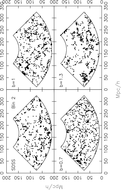
Figure 1: This shows the galaxy distribution in one of the SDSS strip in Bin2 along with some of the simulated slices with bias values as indicated in the panels.

All the sub-samples that we have analyzed are nearly two dimensional. The samples were all collapsed along the thickness (the smallest dimension) to produce 2D galaxy distributions (Figure 1). We use the 2D “Shapefinder” statistic (Bharadwaj et al., 2000) to quantify the average filamentarity of the patterns in the resulting galaxy distribution. A detailed discussion of the method of analysis is presented in Pandey & Bharadwaj (2006) (and references therein), and we highlight only the salient features here. The reader is referred to Sahni, Sathyaprakash,& Shandarin (1998) for a discussion of Shapefinders in three dimensions.

The galaxy distribution is represented as a set of 1s on a 2-D rectangular grid of spacing $1\,h^{-1}{\rm Mpc}\times 1\,h^{-1}{\rm Mpc}$. The empty cells are assigned a value $0$. We identify connected cells having a value 1 as clusters using the ’Friends-of-Friend’ (FOF) algorithm. The filamentarity of each cluster is quantified using the Shapefinder ${\cal F}$ defined as

$${\cal F}=\frac{(P^{2}-16S)}{(P-4l)^{2}}$$ (2)

where $P$ and $S$ are respectively the perimeter and the area of the cluster, and $l$ is the grid spacing. The Shapefinder ${\cal F}$ has values $0$ and $1$ for a square and filament respectively, and it assumes intermediate values as a square is deformed to a filament. We use the average filamentarity

$$F_{2}={\sum_{i}{\cal S}_{i}^{2}{\cal F}_{i}\over\sum_{i}{\cal S}_{i}^{2}}\,.$$ (3)

to asses the overall filamentarity of the clusters in the galaxy distribution.

A problem arises because the distribution of 1s corresponding to the galaxies is rather sparse. Only $\sim 1\%$ of the cells contain galaxies and there are very few filled cells which are interconnected. As a consequence FOF fails to identify the large coherent structures which are visually discernible as filaments in the galaxy distribution (Figure 1). We overcome this problem by successively coarse-graining the galaxy distribution. In each iteration of coarse-graining all the empty cells adjacent to a filled cell are assigned a value $1$. This causes clusters to grow, first because of the growth of individual filled cells, and then by the merger of adjacent clusters as they overlap. Coherent structures extending across progressively larger length-scales are identified in consecutive iterations of coarse-graining. So as not to restrict our analysis to an arbitrarily chosen level of coarse-graining, we study the average filamentarity after each iteration of coarse-graining. The filling factor $FF$ quantifies the fraction of cells that are filled and its value increases from $\sim 0.01$ and approaches $1$ as the coarse-graining proceeds. We study the average filamentarity $F_{2}$ as a function of the filling factor $FF$ (Figure 2) as a quantitative measure of the filamentarity at different levels of coarse-graining. The values of $FF$ corresponding to a particular level of coarse-graining shows a slight variation across the data-sets. In order to combine and compare the results from different data-sets, for each data-set we have interpolated $F_{2}$ to $7$ values of $FF$ at an uniform spacing of $0.1$ over the interval $0.05$ to $0.65$. Further coarse-graining beyond $FF\sim 0.65$ washes away the filaments and hence we do not include this range for our analysis.

For each luminosity bin (Table 1) the seven different strips were used to determine the mean and the variance-covariance matrix for $F_{2}$ as a function of $FF$. This was compared against the mean and the variance-covariance matrix estimated from eighteen simulated data-sets for each value of the bias. Bias values in the range $0.5-2.0$ were considered. For each value of the bias we use the Hotelling’s two sample $T^{2}$ test (Krzanowski, 1990) to test the null hypothesis that the actual values of $F_{2}$ as a function of $FF$, and the predictions of the simulated data belong to the same statistical sample. The $T^{2}$ statistic is defined as

$$T^{2}=(\bar{X_{1}}-\bar{X_{2}})^{\prime}\ \Big{[}\Big{(}\frac{1}{N_{1}}+\frac{1}{N_{2}}\Big{)}S_{p}\Big{]}^{-1}\ (\bar{X_{1}}-\bar{X_{2}})$$ (4)

where $\bar{X_{1}}$ and $\bar{X_{2}}$ are the vectors containing the sample means and $N_{1}=7$ and $N_{2}=18$ are the number of realizations for the data and the simulation respectively. $S_{p}$ is the pooled covariance matrix defined as $S_{p}=\frac{n_{1}S_{1}+n_{2}S_{2}}{n_{1}+n_{2}}$ where $n_{1}=N_{1}-1$, $n_{2}=N_{2}-1$ and $S_{1}$, and $S_{2}$ are the variance-covariance matrix for the data and model respectively. The null hypothesis is rejected for an observed value $T_{0}^{2}>\frac{(n_{1}+n_{2})p}{(n_{1}+n_{2}-p+1)}\,F(p,n_{1}+n_{2}-p+1,1-\alpha)$ where $p=7$ is the number of variables and $F$ is the $F$ distribution. We choose $\alpha=0.05$ which allows us to reject bias values at the $95\%$ confidence level. For each luminosity bin, bias values for which the observed $T_{0}^{2}$ is greater than $T^{2}=24.758$ are rejected with $95\%$ confidence.

We have tested for possible instabilities in inverting the pooled covariance matrix $S_{p}$ arising from the limited number of realisations used to estimate $S_{1}$ and $S_{2}$ (Hartlap, Simon & Schneider, 2006) by repeating the analysis using a smaller number of realisations ($N_{1}=4$ and $N_{2}=10$). The results are found to be unchanged, except for a somewhat larger $b$ range that is accepted with $95\%$ confidence.

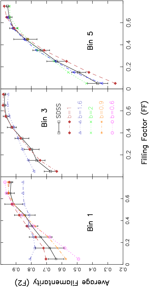
Figure 2: This shows the Average Filamentarity ($F_{2}$) as a function of Filling Factor ($FF$) for every alternate luminosity bins (Table 1). The actual data along with the corresponding results from $\Lambda{\rm CDM}\,\,$N-body simulations are shown for a few representative values of the bias. We use only the range $0.05\leq FF\leq 0.65$ in our analysis.

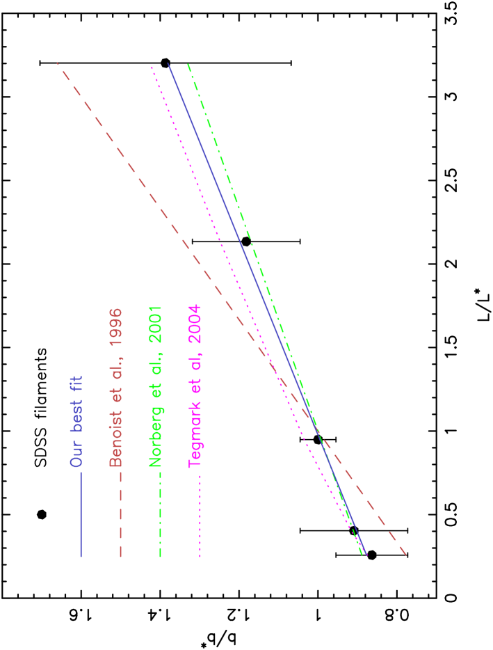
Figure 3: This shows the measured relative bias $\frac{b}{b^{*}}$ of the SDSS galaxies as a function of $\frac{L}{L^{*}}$. The solid curve shows the best fit curve to our data $\frac{b}{b^{*}}=0.833+0.171\frac{L}{L^{*}}$. Fits to data from earlier works are also shown for comparison. The error-bars shown in the figure correspond to $95\%$ confidence intervals.

Table 2: For each luminosity bin this shows the median magnitude and the corresponding bias determined from our analysis. The errors in the bias indicate the $95\%$ confidence interval.

Bin	Median magnitude	Bias
Bin 1	$-18.96$	$0.95\pm 0.1$
Bin 2	$-19.45$	$1.0\pm 0.15$
Bin 3	$-20.38$	$1.1\pm 0.05$
Bin 4	$-21.26$	$1.3\pm 0.15$
Bin 5	$-21.7$	$1.52\pm 0.35$

3 Results and Conclusions

We show results for the Average Filamentarity $F_{2}$ as a function of the Filling Factor $FF$ in Figure 2. Increasing the coarse-graining causes adjacent clusters to connect up into progressively longer interconnected filaments and as a consequence $F_{2}$ increases with $FF$ in the simulations as well as the actual data. At $FF$ in the range $0.5-0.6$ there is a percolation transition where a large fraction of the clusters get interconnected into a single cluster which spans across nearly the entire survey region (Pandey & Bharadwaj, 2005). Continuing the coarse-graining considerably beyond this causes the clusters to thicken and the filamentary patterns are washed away. We restrict our analysis to the range $FF\leq 0.65$ which is slightly beyond the percolation threshold. A point to note here is that the $F_{2}$ curves are sensitive to the area, thickness and number density of the sample (Pandey & Bharadwaj, 2006) which varies considerably across the luminosity bins (Table 1), and in the present analysis it is not meaningful to compare the $F_{2}$ values across the luminosity bins. Considering any one of the luminosity bins in Figure 3, we find that increasing the bias causes $F_{2}$ to go up at low $FF$ whereas the trend is reversed at large $FF$. This can possibly be attributed to the fact that with increasing bias the galaxies get concentrated into more compact regions at the expense of some of the large-scale coherent structures. We also note that the bias dependence of the $F_{2}$ curves is somewhat different from the luminosity dependence (Pandey & Bharadwaj, 2006) which shows a monotonic decrease with increasing luminosity. For each luminosity bin we find that the simulated data-set is consistent with the actual data for only a small range of the bias parameter.

The results of the quantitative comparison of each luminosity bin against the biased simulations are shown in Table 2. It is customary to use $L/L^{*}=10^{-0.4(M-M^{*})}$ to quantify the luminosity of each bin, where $M$ is the median magnitude of the bin and $M^{*}$ has a value $M^{*}=-20.44\pm 0.01$ (Blanton et al., 2003) for the SDSS. The $M^{*}$ galaxies lie in Bin 3 which has a bias value $b^{*}=1.1$. The luminosity dependence ($L/L^{*}$ dependence) of the relative bias $b/b^{*}$ is shown in Figure 3. Fitting a straight line $b/b^{*}=A+B\,(L/L^{*})$ by minimizing

$$\chi^{2}/\nu=\frac{1}{N}\sum^{N}\frac{[(b/b^{*})_{\rm Data}-(b/b^{*})_{\rm Model}]^{2}}{\sigma^{2}_{\rm Data}}$$ (5)

we obtain the best fit values $A=0.833\pm 0.009$ and $B=0.171\pm 0.009$ which gives an acceptable fit with $\chi^{2}/\nu=0.066$. Here we have assumed that at each luminosity bin $\sigma_{\rm Data}$ is half the corresponding $95\%$ confidence interval. Note that such a low value of $\chi^{2}/\nu$ is unlikely (probability $<2.5\%$) if the errors in the different luminosity bin are uncorrelated and have a normal distribution. It is possible that these assumptions do not hold, and a further possibility is that using half the $95\%$ confidence interval overestimates $\sigma_{\rm Data}$.

We find that our best fit luminosity bias relation is very close to those proposed by Norberg et al. (2001) and Tegmark et al. (2004), both of which provide acceptable fits to our data with $\chi^{2}/\nu=0.189$ and $1.154$ respectively. The luminosity bias relation obtained by Peacock et al. (2001) through fitting the Benoist et al. (1996) data is considerably steeper. Their luminosity bias relation shows considerable deviations from our data at both the low and high luminosity ends and is ruled out with $\chi^{2}/\nu=4.697$. This is consistent with Norberg et al. (2001) who find considerable deviations between their data and the Benoist et al. (1996) data at high luminosities.

The observed luminosity bias relation is an useful input for models of galaxy formation. Hierarchical models of galaxy formation (e.g. White et al. 1987) generally assume the brighter galaxies to be associated with the more massive dark matter halos which have a stronger clustering. The semi-analytic model of galaxy formation of Benson et al. (2001) is consistent with the observed luminosity bias relation (Norberg et al., 2001). Zehavi et al. (2005) show that the halo model with suitably chosen parameters can correctly predict the observed luminosity dependence. We note that the focus of much of these works has been on the luminosity dependence of the two-point statistics. The largest currently available implementation of a semi-analytic model of galaxy formation (The Millennium Run, Springel et al. 2005) fails to correctly predict the luminosity dependence of the filamentarity for the brightest galaxies (Pandey & Bharadwaj, 2006). Finally, it is interesting that our analysis which uses a global property of the galaxy distribution, namely its morphology, predicts the same luminosity bias relation as determined from the two point statistics.

4 Acknowledgment

SB would like to acknowledge financial support from the Govt. of India, Department of Science and Technology (SP/S2/K-05/2001). BP would like to thank the CSIR, Govt. of India for financial support through a Senior Research fellowship. The SDSS DR4 data was downloaded from the SDSS skyserver http://skyserver.sdss.org/dr4/en/.

Funding for the creation and distribution of the SDSS Archive has been provided by the Alfred P. Sloan Foundation, the Participating Institutions, the National Aeronautics and Space Administration, the National Science Foundation, the U.S. Department of Energy, the Japanese Monbukagakusho, and the Max Planck Society. The SDSS Web site is http://www.sdss.org/.

The SDSS is managed by the Astrophysical Research Consortium (ARC) for the Participating Institutions. The Participating Institutions are The University of Chicago, Fermilab, the Institute for Advanced Study, the Japan Participation Group, The Johns Hopkins University, the Korean Scientist Group, Los Alamos National Laboratory, the Max-Planck-Institute for Astronomy (MPIA), the Max-Planck-Institute for Astrophysics (MPA), New Mexico State University, University of Pittsburgh, Princeton University, the United States Naval Observatory, and the University of Washington.

References

- Abazajian et al. (2003) Abazajian, K., et al. 2003, AJ, 126, 2081
- Abazajian et al. (2004) Abazajian, K., et al. 2004, AJ, 128, 502
- Adelman-McCarthy et al. (2006) Adelman-McCarthy, J. K., et al. 2006, ApJS, 162, 38
- Benoist et al. (1996) Benoist, C., Maurogordato, S., da Costa, L.N., Cappi, A., & Schaeffer, R., 1996, ApJ, 472, 452
- Benson et al. (2001) Benson, A. J., Frenk, C. S., Baugh, C. M., Cole, S., & Lacey, C. G. 2001, MNRAS, 327, 1041
- Bharadwaj et al. (2000) Bharadwaj, S., Sahni, V., Sathyaprakash, B. S., Shandarin, S. F., & Yess, C. 2000, ApJ, 528, 21
- Bharadwaj, Bhavsar & Sheth (2004) Bharadwaj, S., Bhavsar, S. P., & Sheth, J. V. 2004, ApJ, 606, 25
- Bharadwaj & Pandey (2004) Bharadwaj, S., Pandey, B. 2004, ApJ, 615, 1
- Blanton et al. (2003) Blanton, M. R., et al. 2003, ApJ, 592, 819
- Cole, Hatton & Weinberg (1998) Cole, S., Hatton, S., Weinberg, D. H., & Frenk, C. S. 1998, MNRAS, 300, 945
- Colless et al. (2001) Colless, M. et al. (for 2dFGRS team) 2001, MNRAS, 328, 1039
- da Costa et al. (1994) da Costa, L.N., et al. 1994, ApJL, 424, L1
- Davis et al. (1988) Davis, M., Meiksin, A., Strauss, M.A., da Costa, L.N., & Yahil, A., 1988, ApJ, 333, L9
- Dekel & Lahav (1999) Dekel, A. & Lahav, O. 1999, ApJ, 520, 24
- Guzzo et al. (1997) Guzzo, L., Strauss, M.A., Fisher, K.B., Giovanelli, R., & Haynes, M.P., 1997, ApJ, 489, 37
- Hamilton (1998) Hamilton, A.J.S., 1988, ApJ, 331, L59
- Hartlap, Simon & Schneider (2006) Hartlap, J., Simon, P., Schneider, P. 2006, A&A, in press, astro-ph/0608064
- Hawkins et al. (2003) Hawkins, E., et al.2003, MNRAS,346,78
- Krzanowski (1990) Krzanowski, W.J. 1990, Principles of Multivariate Analysis: A User’s Perspective, Oxford: Clarendon press, 1990
- Loveday et al. (1995) Loveday, J., Maddox, S.J., Efstathiou, G., & Peterson, B.A. , 1995, ApJ, 442, 457
- Norberg et al. (2001) Norberg, P., et al. 2001, MNRAS, 328, 64
- Pandey & Bharadwaj (2005) Pandey, B. & Bharadwaj, S. 2005, MNRAS, 357, 1068
- Pandey & Bharadwaj (2006) Pandey, B. & Bharadwaj, S. 2006, MNRAS, 372, 827
- Park, Vogeley, Geller & Huchra (1994) Park, C., Vogeley, M.S., Geller, M.J., & Huchra, J.P., 1994, ApJ, 431,569
- Peacock et al. (2001) Peacock, J. A., et al. (the 2dFGRS team) 2001, Nature, 410, 169
- Sahni, Sathyaprakash,& Shandarin (1998) Sahni, V., Sathyaprakash, B. S., & Shandarin, S. F. 1998, ApJL, 495, L5
- Seljak et al. (2005) Seljak, U., et al. 2005, Physical Review D, 71, 043511
- Shectman et al. (1996) Shectman, S. A.,Landy, S. D., Oemler, A., Tucker, D. L., Lin, H., Kirshner, R. P., & Schechter, P. L. 1996, ApJ, 470, 172
- Spergel et al. (2003) Spergel, D. N. et al. 2003, ApJ, 148, 175
- Spergel et al. (2006) Spergel, D. N. et al. 2006, submitted to ApJ, (astro-ph/0603449)
- Springel et al. (2005) Springel et al. 2006, Nature, 435, 629
- Tegmark et al. (2004) Tegmark, M., et al. 2004, ApJ, 606, 702
- Verde et al. (2002) Verde, L., et al. 2002, MNRAS, 335, 432
- White, Tully & Davis (1988) White, S.D.M., Tully, R.B., & Davis, M., 1988, ApJ, 333, L45
- White et al. (1987) White, S.D.M., Davis, M., Efstathiou, G., Frenk, C.S., 1987, Nature, 330, 351
- York et al. (2000) York, D. G., et al. 2000, AJ, 120, 1579
- Zehavi et al. (2005) Zehavi, I., et al. 2005, ApJ, 630, 1