The first direct detection of a gravitational $\mu$-lens toward the Galactic Bulge

Abstract

We present a direct detection of the gravitational lens that caused the microlensing event MACHO-95-BLG-37. This is the first fully resolved microlensing system involving a source in the Galactic bulge, and the second such system in general. The lens and source are clearly resolved in images taken with the High Resolution Channel of the Advanced Camera for Surveys on board the Hubble Space Telescope (HST) $\sim 9$ years after the microlensing event. The presently available data are not sufficient for the final, unambiguous identification of the gravitational lens and the microlensed source. While the light curve models combined with the high resolution photometry for individual objects indicate that the source is red and the lens is blue, the color-magnitude diagram for the line of sight and the observed proper motions strongly support the opposite case. The first scenario points to a metal-poor lens with mass $M\approx 0.6M_{\odot}$ at the distance $D_{\rm l}\approx 4$ kpc. In the second scenario the lens could be a main-sequence star with $M=0.8$–$0.9M_{\odot}$ about half-way to the Galactic bulge or in the foreground disk, depending on the extinction.

1. Introduction

Gravitational microlensing of stars within the Local Group of galaxies (Paczyński 1996) directly probes both luminous and dark matter concentrations along the line of sight. Over the past decade microlensing surveys have continued to enable observations with far-reaching implications, such as constraints on the fraction and content of Galactic dark matter (e.g. Alcock et al. 1996, 1998, 2001), discovery and characterization of exo-planet systems (Bond et al. 2004; Udalski et al. 2005; Beaulieu et al. 2006; Gould et al. 2006), and measurements of the fundamental properties of stars and their evolutionary end points (Bennett et al. 2002; Abe et al. 2003; Gould et al. 2004). Unfortunately, while the light curve of a microlensing event provides the key discovery signature, it is insufficient to solve uniquely for the mass, the distance and the relative transverse velocity of the lens. As a result, out of a few thousand events discovered to date, only a handful allowed the mass of the lens to be measured (An et al. 2002; Gould et al. 2004; Jiang et al. 2004).

In the case of microlensing by a luminous body (a star) the basic degeneracy of the model can be broken by directly observing both the lens and the source. The difficulty with this approach, however, is inherent in the geometry of microlensing that implies milli-arcsecond separations between the lens and source components during the event. So far MACHO-LMC-5 was the only microlensing event for which the lensing body has been resolved (Alcock et al. 2001). The lens that gravitationally magnified the source in the Large Magellanic Cloud turned out to be a nearby M dwarf in the Galactic disk (Drake et al. 2004; Gould et al. 2004). Bennett et al. (2006) demonstrated the presence of a bright lens component in the planetary microlensing event OGLE-2003-BLG-235/MOA-2003-BLG-53 and estimated the mass of the host star using the centroid shift of the combined light.

Here we report a direct detection and mass measurement of the gravitational lens responsible for the MACHO-95-BUL-37 event—the first fully resolved microlensing system involving a Galactic bulge source, and the second such system in general.

2. Microlensing event MACHO-95-BLG-37

The event was discovered by the MACHO collaboration as a single and apparently achromatic brightening of object 109.20635.2193 in their photometric monitoring database of the Galactic bulge (see Thomas et al. 2005). The object is quite faint ($V\sim 20$ mag) and located in one of the densest fields covered by the survey: equatorial (J2000) and Galactic coordinates $(\alpha,~{}\delta)$=(18h04m34.44s, $-$28${}^{\circ}25^{\prime}33.7^{\prime\prime}$),($l,~{}b$)=(2^∘.54, $-$3^∘.33). The location of the MACHO-95-BLG-37 event was one of the targets in our proper motion mini-survey of the Galactic bulge (Kozłowski et al. 2006). Each of the 35 fields in the mini-survey was centered on a microlensed source and was covered by two Hubble Space Telescope (HST) pointings taken several years apart. Using several relatively isolated stars we could co-register the HST and ground-based MACHO images to within $0.1\arcsec$ and unambiguously identify microlensed sources, even in the presence of additional stars that were only resolved in the HST images.

In the case of MACHO-95-BLG-37 we found that not only is the microlensed source accompanied by another very close star with comparable brightness, but also that the relative proper motion of the two components places them within $2.6\pm 3.5$ mas of each other on 21 September 1995 (HJD 2449982.3) when the microlensing event took place. The prior probability that the blend is a random coincidence is very small, so we have a clear indication that the companion source is actually the gravitational lens that caused the event of 1995. Before we begin a detailed investigation of this finding (§§ 3–5) we first describe the available data and basic data reductions.

2.1. HST astrometry and photometry

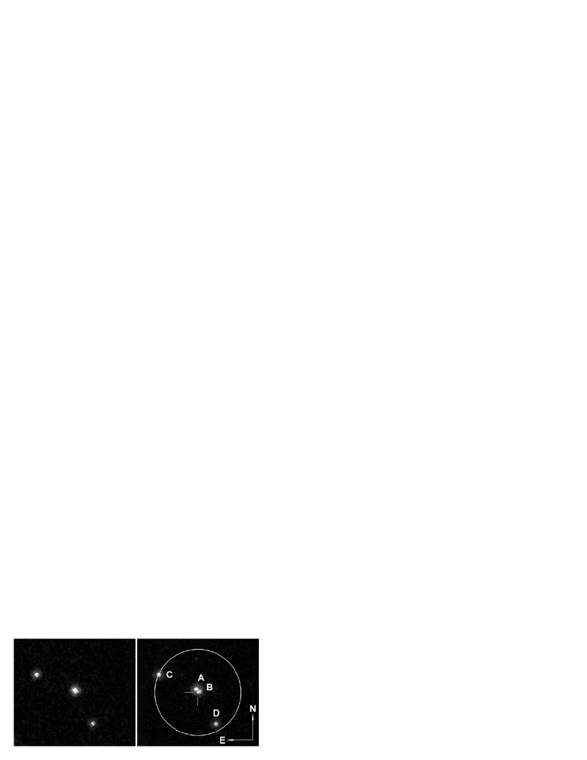
Figure 1.— HST images of the MACHO-95-BLG-37 event location. The first epoch WFPC2/PC image (left) and the second epoch ACS/HRC image (right) were taken, respectively, 3.71 and 8.95 yr after the maximum light. The relative trajectory of stars A and B places them within 2.6 mas of each other at the time of the microlensing event. The circle shows a seeing disk characteristic of the ground-based MACHO survey (FWHM$\simeq 2^{\prime\prime}\hskip-2.0pt.1$). The crosshair indicates the unbiased centroid of the lensed light from difference imaging.

A detailed description of the relevant HST data was published in Kozłowski et al. (2006) and only the essential facts are repeated here. The first and second epoch images were collected, respectively, 3.71 and 8.95 yr after the event. The first pointing employed the Planetary Chip (PC) of the Wide Field Planetary Camera 2 (WFPC2) instrument, and provided (nearly) simultaneous color information in both $V$ and $I$ photometric bands using F555W and F814W filters. During the second pointing we used the High Resolution Channel (HRC) of the Advanced Camera for Surveys (ACS) and obtained high signal-to-noise ratio (S/N) imaging in the F814W filter only. In each case we co-added all suitable F555W and F814W images for a given epoch. The field of view covered by the ACS/HRC and WFPC2/PC detectors is similar ($29\arcsec\times 26\arcsec$ and $35\arcsec\times 35\arcsec$, respectively), but not the pixel size ($25$ versus $45.5$ mas). At the HST resolution the MACHO database object associated with the microlensing source was immediately revealed to be a composite of four unresolved stars, which we label A through D (Fig. 1).

The magnitudes and positions of stars A–D were extracted from the fits of stellar profiles. The local point spread function (PSF) models were generated using the TINYTIM software (Krist 1993, 1995) and interpolated with bi-cubic splines. For all model fitting we used the MINUIT package. Stars A and B have overlapping profiles and required a special model with two PSF components fitted simultaneously. A small section of the ACS/HRC image was fitted first, providing an unbiased value of the second epoch separation between the two components and a good handle on the flux ratio in the $I_{\rm F814W}$-band. The flux ratio was then fixed at the second epoch value for the purpose of fitting the $I_{\rm F814W}$-band WFPC2/PC image and obtaining the first epoch astrometry. Finally, the $(V-I)$ colors of stars A and B were established by fitting the $V_{\rm F555W}$-band image using a model with variable flux ratio and the blend separation fixed at the value taken from the $I_{\rm F814W}$-band fit for the same epoch. The resulting astrometric and photometric measurements are given in Tables 1 and 2. Note that in the $V$-band the only available high resolution imaging comes from the relatively shallow first epoch WFPC2/PC observation, so the A/B flux ratio is poorly constrained and the errors in $V$ and $(V-I)$ are relatively large for these two stars. In the $I$-band, however, we have an accurate measurement of the flux ratio from ACS/HRC that allowed us to eliminate a degenerate free parameter from the double PSF fit of the WFPC2/PC data. This explains why the astrometric accuracy for the first epoch is actually better than for the second epoch, despite a larger pixel size and a much smaller separation between stars A and B in the WFPC2/PC images compared to the ACS/HRC data. Using simulated images we found that our first epoch astrometry is biased by about 1.5% toward lower separations. We could not find a better procedure that would eliminate this effect, so a post-factum correction was included in the WFPC2/PC data reported in Table 1.

2.2. Microlensing light curve revisited

Figure 2.— Light curve of the MACHO-95-BLG-37 event from our Difference Image Analysis of data in the public MACHO database. A significant color change near the peak magnification indicates that the microlensed source is redder than the unresolved composite of stars A, B, C and D from Fig. 1.

The MACHO-95-BLG-37 event was recorded in a faint star subject to intense crowding, and therefore the standard light curve in the MACHO photometric database has a very low S/N. In order to reduce the uncertainties of the microlensing parameters derived from light curve modeling we performed Difference Image Analysis (DIA; Alard & Lupton 1998; Alard 2000; Woźniak 2000) on the original ground-based images, i.e. on the simultaneous two-color imaging data collected by the MACHO survey. The PSF matching and photometric solutions were confined to a $2^{\prime}\hskip-2.0pt.5\times 2^{\prime}\hskip-2.0pt.5$ region around the source (approximately $256\times 256$ pixels). After discarding observations outside the relevant time interval and rejecting a small fraction of frames with bad seeing we considered a total of 132 images in each of the MACHO photometric bands $b_{\rm M}$ and $r_{\rm M}$. High S/N reference images were constructed by co-adding 9 good quality images with a well-behaved PSF. From a series of difference frames in which the source was significantly magnified we derived an unbiased centroid of the lensed light that clearly points to the pair of stars A and B when transformed to the ACS/HRC coordinates (Fig. 1). One of these two stars must then be the microlensed source.

Table 1HST astrometry

Instrument		Epoch	$t-t_{0}$	$\Delta\alpha$	$\Delta\delta$
		(yr)	(yr)	(mas)	(mas)
WFPC2/PC		1999.43	3.71	$-29.9\pm 1.3$	$-24.9\pm 1.3$
ACS/HRC		2004.67	8.95	$-74.5\pm 1.6$	$-63.1\pm 1.6$

Note. — $\Delta\alpha$, $\Delta\delta$ are positions of star B relative to star A (Fig. 1) in a Cartesian reference frame aligned with the local equatorial coordinates. The moment of maximum light $t_{0}$ corresponds to HJD = 2449982.3 (Epoch 1995.72).

Table 2HST photometry

Star	$V_{\rm F555W}$	$I_{\rm F814W}$	$(V-I)$	$f_{V}$	$f_{I}$
	(mag)	(mag)	(mag)
A	$20.24\pm 0.08$	$18.45\pm 0.02$	1.79	0.28	0.35
B	$20.30\pm 0.08$	$19.07\pm 0.04$	1.23	0.26	0.19
C	$20.29\pm 0.03$	$18.66\pm 0.03$	1.63	0.27	0.28
D	$20.63\pm 0.04$	$19.18\pm 0.04$	1.45	0.19	0.18

Note. — $f_{V},f_{I}$ are fractional contributions to the total flux

The reference flux in each band was derived from a comparison between our differential fluxes and conventional PSF photometry obtained with the Dophot software (Schechter et al. 1993) running in a fixed-position mode with the input object lists based on our deep reference images. Stars C and D could not be properly deblended, even using fixed HST positions transformed to the template coordinates. The template position of the A–D composite was set to the mean ACS/HRC position of stars A and B. We selected 31 calibration images per photometric band with the best overall seeing, background and transparency. In seven of these images the source was visibly magnified. The statistical uncertainty of the reference flux is 8% in $b_{\rm M}$ and 9% in $r_{\rm M}$. The background level estimated by the Dophot algorithm in a crowded field is somewhat sensitive to the assumed shape of the PSF (especially in the wings). In our case of a very faint object near the detection limit set by the source confusion we find that the systematic uncertainty in the reference flux can easily reach 10%. This generic problem is partially alleviated by the fact that the systematics are similar in both filters and source blending must always be considered in the analysis of individual light curves in crowded fields.

The final light curves (Fig. 2) were shifted to the instrumental $b_{\rm M}$, $r_{\rm M}$ scale of the MACHO database using a median offset for a few tens of bright stars near the location of the MACHO-95-BLG-37 event and transformed to approximately standard $V_{\rm M},R_{\rm M}$ magnitudes following Popowski et al. (2005). We also determined transformations between $V_{\rm M},R_{\rm M}$ and the standard $V,I$ magnitudes:

$$\begin{array}[]{ccr}V_{\rm M}&=&V+(0.05\pm 0.11)(V-I)+(0.01\pm 0.20),\\ R_{\rm M}&=&I+(0.62\pm 0.10)(V-I)-(0.17\pm 0.18).\end{array}$$ (1)

Hereafter, the subscript is omitted and MACHO filters are implied for $V,R$ photometry. The overall quality of the $V$-band light curve is lower compared to that in the $R$-band due to occasional pixel level defects in the $b_{\rm M}$ frames that were clearly visible in the difference images.

3. Microlensing light curve models

The first step is to obtain the basic microlensing parameters such as the time-scale $t_{\rm E}$, the dimensionless impact parameter $u_{0}$, the moment of the peak brightness $t_{0}$, and the baseline magnitudes $m_{V,R}$. In order to preserve consistent color information, both $V$- and $R$-band light curves were fitted simultaneously with a simple microlensing model that allows for flux blending (source fractions $f_{\rm s}<1$). The data point at $t=1016.9$ days is a moderate outlier in the $V$-band light curve (Fig. 2) and is rejected in all analyses. The change in $\chi^{2}$ due to this cosmetic change is not significant and none of our conclusions are affected. The resulting best fit model is given in Table 3 and provides a marginally acceptable fit (reduced $\chi^{2}_{\nu}=1.49$ for $\nu=255$ degrees of freedom).

Table 3Microlensing light curve model

Parameter	Value	Error
$t_{0}$ (days)	982.3	0.3
$t_{\rm E}$ (days)	25.2	4.2
$u_{0}$	0.37	0.10
$f_{{\rm s},V}$	0.33	0.12
$f_{{\rm s},R}$	0.38	0.14
$m_{V}$ (mag)	19.314	0.005
$m_{R}$ (mag)	18.545	0.003
$\chi^{2}_{\nu}$	1.490	$\cdots$
$\nu$	255	$\cdots$

Note. — Maximum magnification is at $t_{0}$ days after HJD = 2449000.

3.1. Colors

Using different parameterizations of the model equivalent to the one in Table 3, we obtained the source/blend colors and the color difference with the error bounds that fully account for covariance: $(V-R)_{\rm s}=0.92\pm 0.04$, $(V-R)_{\rm b}=0.68\pm 0.04$ and $\Delta(V-R)_{\rm s,b}=(V-R)_{\rm s}-(V-R)_{\rm b}=0.24\pm 0.06$. This corresponds to a positive color shift during the event $\Delta(V-R)_{\rm event}\simeq+0.06$ mag and indicates that the source is redder than the blend. However, it must be emphasized that the measurement of the reference flux for our light curves poses a significant challenge given the limitations of the available archival data (§ 2.2). Both $(V-R)_{\rm b}$ and $\Delta(V-R)_{\rm s,b}$ are subject to the systematics of the reference flux in two bands. The value of $(V-R)_{\rm s}$, on the other hand, is more reliable, because it is constrained by the magnified portion of the light curve, even if the reference fluxes are not known. This is best seen from the model of the simultaneous two-color DIA light curve written as $\Delta F(t)=F_{\rm s}\times A(t)+F_{0}$ in each band, where $A(t)$ is the magnification factor and $F_{0}<0$ if the source is effectively magnified in the reference image. Although in most cases the source flux $F_{\rm s}$ is poorly constrained in both colors, the error bounds on the ratio $F_{{\rm s},V}/F_{{\rm s},R}$ are relatively tight due to covariance and, most importantly, independent of the flux offsets. Therefore, the derived value of $(V-R)_{\rm s}$ only depends on the global calibration of flux units for the reference images, which can be done much more reliably using bright isolated stars. In conjunction with the HST photometry, the source color information will be crucial to deciding the identity of the microlensed source, and therefore the lens (§ 4.1).

3.2. Parallax constraints

The ground-based microlensing light curve provides useful constraints on the acceleration term in the observed trajectory of the lens relative to the source. In the case of a short, low-magnification microlensing event such as MACHO-95-BLG-37 we can only obtain one-dimensional information (Gould et al. 1994). Following the geocentric formalism of Gould (2004), we introduce into the model the dimensionless microlensing parallax vector $\mbox{\boldmath$\pi$}_{\rm E}$, where $\pi_{\rm E,\parallel}$ is the component of $\mbox{\boldmath$\pi$}_{\rm E}$ opposite the direction of the projected position of the Sun at the peak of the event. We find that $\pi_{\rm E,\parallel}=0.07^{+0.65}_{-0.46}$, while $\pi_{\rm E,\perp}$ remains unconstrained, i.e. there is no detectable parallax. There are two observations during the event (at $t=967.9$ and $t=996.9$ days) with atypically low $V$-band fluxes and relatively large error bars compared to the adjacent measurements. Without these two data points we get $\pi_{\rm E,\parallel}=0.00^{+0.67}_{-0.45}$ and the apparent weak asymmetry of the best fit model goes away. In § 4.1 this constraint is improved using ${\it HST}$ photometry and in § 4.2 combined with the ${\it HST}$ astrometry to place the limits on the relative source-lens parallax $\pi_{\rm rel}$.

4. Resolution of the microlensing system into lens and source

The fundamental difficulty with resolving a lens detected through time-variable magnification is that its apparent separation from the source is below the HST resolution for months or even years after the event. In the case of MACHO-95-BLG-37 (and similarly for MACHO-LMC-5) this problem is greatly reduced due to the rather large relative motion of stars A and B (§ 2.1). High precision HST astrometry at two epochs well after the peak magnification allowed us to calculate a very accurate relative trajectory of star B with respect to star A. Simply connecting the two measurements in Table 1 we get:

$$\mathbf{r}(t)=\mathbf{r}(t_{1}){(t_{2}-t)\over(t_{2}-t_{1})}+\mathbf{r}(t_{2}){(t-t_{1})\over(t_{2}-t_{1})},$$ (2)

where $\mathbf{r}=(\Delta\alpha,\Delta\delta)$ is the relative position with measurements available at $t_{1}=3.71$ and $t_{2}=8.95$ yr. The separation at the peak of the event ($t=0$) is then:

$(\Delta\alpha_{0},\Delta\delta_{0})=(1.6\pm 2.5,~{}2.1\pm 2.5)~{}{\rm mas}.$

These values are fully consistent with a model in which the two stars are the source and lens, and which predicts a very low value of the two-dimensional separation $r_{0}=r(0)$. There are two alternative possibilities: either one of the members of the pair is a random interloper, or it is a companion to either the lens or the source. The first possibility is ruled out by the following argument: In the sky region under consideration the density of stars is 0.085 and 0.176 per square arcsecond for stars brighter than $I=18.45$ and 19.07 mag, respectively. The corresponding Poisson probabilities of a random alignment within 2.6 mas at the time of the event are $1.8\times 10^{-6}$ and $3.7\times 10^{-6}$, respectively, i.e. very low. The other case, of one of the two detected stars being a companion to either the lens or the source, can also be ruled out. It is clear is that one of the two stars must be the source. Furthermore, the rapid relative proper motion excludes the possibility that the second star is a companion of the source (the implied binary motion will be too high, about 400 km/s at a distance of 8 kpc). Thus we only need to consider the possibility that one of the stars is a companion of an unseen dark lens, with a separation of about 2.6 mas between them (recall that the lens is almost perfectly aligned with the lensed source at the peak). This is about $b\approx 3.5$ Einstein radii (for $\theta_{\rm E}=0.75\pm 0.13$ mas, see §4.2). We can approximately model the perturbation of the luminous star on the dark lens as a Chang-Refsdal lens (Chang & Refsdal 1984). The shear induced by the luminous star at the position of the dark lens would be $\gamma=q/b^{2}\approx 0.08$, where $q$ is the mass ratio of the luminous companion to the dark lens. The short $t_{\rm E}$ does not favor a massive dark lens such as a black hole and neutron star, and so the mass ratio $q$ is likely larger than one. The caustics will have a size roughly $2\gamma/\sqrt{1-\gamma}\approx 2q/b^{2}\sim 0.16$ (e.g. Mao 1992). The caustics size is comparable to the measured impact parameter ($u_{0}\sim 0.37$), which would introduce a strong asymmetry in the light curve for most trajectories (not seen in the observed low S/N light curves). Hence we regard the ‘dark’ lens scenario as not very likely. The bright lens hypothesis is thus favored and we conclude that the source and lens system involved in the MACHO-95-BLG-37 microlensing event consists of stars A and B from Figure 1 (in an order still to be determined). Our subsequent arguments are based on that assumption.

4.1. Identifying the lens

To find out which member of the candidate pair of stars is the lens, we can make use of the observed color change during the event and the fact that gravitational lensing is achromatic. In Figure 3 we plot the color-magnitude diagram (CMD) of the stellar field around MACHO-95-BLG-37 and stars A–D from Figure 1. The light curve in Figure 2 reflects the integrated flux of the four stars (unresolved in ground-based images). From the observed color increase $\Delta(V-R)_{\rm event}\simeq+0.06$ mag near the peak magnification we infer that the microlensed source is redder than the composite. Although the $(V-R)$ colors were not measured individually for stars A–D, it is very unlikely that the ordering of the $(V-I)$ and $(V-R)$ colors is different. Stars A and B are, respectively, the reddest and the bluest components of the blend, so the color shift points to star A as the source. This is entirely in agreement with the source color $(V-R)_{\rm s}=0.92\pm 0.04$ mag and the color difference $(V-R)_{\rm s,b}=0.24\pm 0.06$ mag between the source and the rest of the blend found in § 3.1. Equation (1) implies HST $(V-I)_{\rm s}\simeq 1.7$ mag, also consistent with the HST photometry of star A. Thus, based on the light curve evidence, star B must be the lens, because star A is the microlensed source. However, in § 5 we show that the physical interpretation of the CMD and kinematic data strongly argues against this result.

In principle, the HST photometry provides an additional test of these possibilities because we can transform the measurements to the MACHO system and obtain a constraint on the source magnitudes $V=20.34\pm 0.09,R=19.38\pm 0.05$ assuming star A and $V=20.37\pm 0.11,R=19.66\pm 0.08$ assuming star B (including the variance and covariance in transformation coefficients). Unfortunately, the difference $\Delta\chi^{2}\simeq 0.1$ between the models with stars A and B as the source is completely insignificant. An additional problem is that the contributions of stars A–D to the blend are not known very well. In order to match the total MACHO baseline magnitudes (§ 2.2) we would have to make the transformed HST fluxes of all four stars fainter by 10–15%, depending on the photometric band, and then still assume that only about half of the flux in stars C and D is effectively added to the total flux of stars A and B. This is not surprising knowing that stars C and D are near the edge of the FWHM disk of stars A and B (Fig. 1)—yet they are too faint to be deblended—and that in ground-based microlensing images the “sky” level is set by a featureless continuum of merging stars. Overestimating the background by a mere few counts makes stars near the detection limit appear 0.1–0.2 mag fainter. The weights are probably slightly different in each photometric band due to details such as the orientation of stars C and D with respect to the PSF that is never perfectly round. Nevertheless, it is still useful to perform a microlensing light curve fit with a single additional “measurement” of the source magnitude, i.e. effectively constrain $f_{\rm s}$. Compared to the results in § 3.2, the error bounds on the dimensionless parallax are improved, yielding $\pi_{\rm E,\parallel}=0.0\pm 0.4$ for any reasonable set of flux weights.

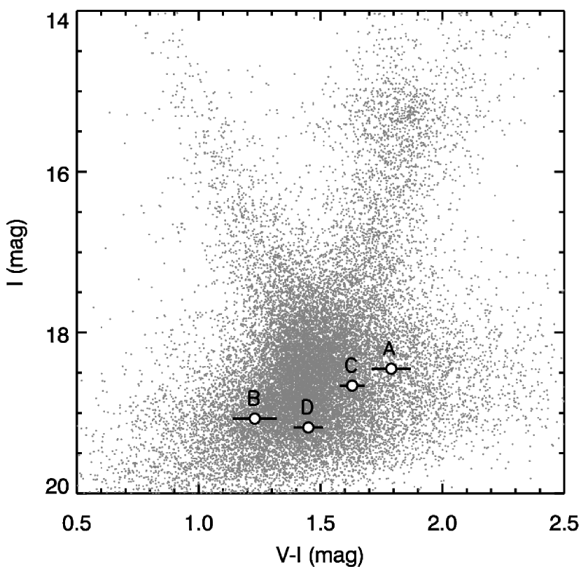
Figure 3.— Color-magnitude diagram (CMD) of stars around the MACHO-95-BLG-37 event location. The HST photometry of stars A–D from Fig. 1 (open circles) is plotted against the average bulge and disk population along the line of sight (OGLE-II data; Udalski et al. 2002).

4.2. Proper motion, Einstein ring radius and relative parallax

The relative proper motion $\mu_{\rm rel}$ of the lens with respect to the source provides further clues about the physics of the event. For the case at hand, a robust value of $\mu_{\rm rel}$ can be derived from the HST astrometry alone. If we ignore the parallax and approximate $u_{0}=0$, we find $\mu_{\rm rel}=10.85\pm 0.16{\rm{\rm\,mas}}\,{\rm yr}^{-1}$ and the position angle $\phi=229.83\pm 0.84$ deg (North through East). Allowing for a finite impact parameter makes no difference to $\mu_{\rm rel}$, changes $\phi$ by a mere $0.4$ deg, and predicts the peak brightness a couple of months after the actual event, consistent within 1$\sigma$ uncertainties. Including the parallax also has a negligible influence on the trajectory. Thus the Einstein radius can be estimated as $\theta_{\rm E}=\mu_{\rm rel}t_{\rm E}=0.75\pm 0.13$ mas.

The direction of the dimensionless parallax vector $\mbox{\boldmath$\pi$}_{\rm E}$ is the same as the direction of the lens-source relative proper motion. The component $\pi_{\rm E,\parallel}$ that points away from the projected position of the Sun is almost perfectly due East, since the event peaked on 21 September. Using results from § 3.2 and § 4.1 we can immediately estimate $\pi_{\rm E}=|\pi_{\rm E,\parallel}(\sin\phi)^{-1}|<0.53$, and set an upper limit on the relative lens-source parallax, $\pi_{\rm rel}=\pi_{\rm E}\theta_{\rm E}\lesssim 0.3$ mas.

5. Microlensing scenarios and the lens mass

Table 4HST kinematics of stars A and B

star	$\mu_{\rm l}$	$\mu_{\rm b}$
	(${\rm{\rm\,mas}}\,{\rm yr}^{-1}$)	(${\rm{\rm\,mas}}\,{\rm yr}^{-1}$)
A	$6.9\pm 0.3$	$-0.2\pm 0.3$
B	$-3.8\pm 0.4$	$3.7\pm 0.4$

Note. — Proper motions are expressed in an average star reference frame as defined in Kozłowski et al. (2006).

The value of the source color derived in § 4.1 favors a scenario in which star A is the source and star B is the lens. However, as we show in this section, such arrangement is very unlikely in the context of the CMD (Fig. 3) and proper motions measured relative to the Galactic bulge (Table 4). Although the extinction-to-reddening ratio in the direction of the event is abnormally low, the reddening anomaly cannot explain the conflict. After Sumi (2004), we adopt the reddening coefficient $R_{\rm VI}=A_{\rm V}/E_{\rm V-I}=1.98$ and the total bulge extinction $A_{\rm V}=1.54$ mag. In the following discussion we consider both source star cases in some detail and then use the measurement of $\theta_{\rm E}$ from § 4.2 to constrain the mass of the lens.

5.1. Blue lens scenario

First we attempt to reconcile all available data with the evidence in § 4.1 that the source is red. Given its red color, star A is too faint to be a giant and too bright to be on the main sequence in the Galactic bulge. If it were a giant several magnitudes behind the bulge, it could in principle belong to the Sgr dwarf galaxy, but its observed proper motion is not consistent with Sgr (Ibata et al. 1997). More likely, star A is a dwarf in the foreground disk at a distance of $\sim 2.5$ kpc and behind most of the extinction. Then, if star B is indeed the lens, it must be in front of star A, and the only simple solution is that the lens is a nearby white dwarf at $\sim 100$ pc or so. Unfortunately, this exciting possibility is ruled out by the parallax constraint $\pi_{\rm rel}<0.3$ mas (§ 4.2), as it predicts $\pi_{\rm rel}\sim 10$ mas.

The location of star A in the CMD is still marginally consistent with a faint subgiant on the far side of the bulge subject to $\sim 0.2$ mag of extra reddening compared to the general population. But there is little support for that, since the CMD shows a compact red clump and indicates a very uniform extinction across this field (c.f. the extinction map of Sumi 2004). The observed kinematics would also be very unusual for this scenario with star A showing a 7 ${\rm{\rm\,mas}}\,{\rm yr}^{-1}$ disk-like prograde motion in the plane and star B moving at a $\sim 135^{\circ}$ inclination. One could still argue that star B is a low metallicity halo subdwarf to explain its motion and dramatically increase the $A_{\rm V}$ prediction, but there is simply too much fine tuning to consider this a reliable solution.

5.2. Red lens scenario

The properties of both stars are much easier to explain if we dismiss for a moment the source color evidence from § 4.1 and assume that star B is the source and star A is the lens. In this case star B is most likely in the bulge, where its absolute magnitude and color would be approximately $M_{\rm I}=3.6,(V-I)_{0}=0.4$ assuming a red clump at $I_{\rm RC}=15.3,(V-I)_{\rm RC}=1.8$ in Figure 3 and adopting $M_{\rm I,RC}=-0.2,(V-I)_{\rm 0,RC}=1.0$ (Udalski 2000). So the source fits the properties of a metal-poor star near the turnoff point in the bulge, and the observed proper motion is fully consistent with this picture. Then star A must be the lens and can be placed on the main sequence at a distance of $\sim 4$ kpc, where it would follow the Galactic rotation near the plane and move a few ${\rm{\rm\,mas}}\,{\rm yr}^{-1}$. Again, the observed kinematics support this scenario.

5.3. The lens mass estimates

Any acceptable scenario for the lens must satisfy the constraint on microlensing geometry set by the measurement of the Einstein radius $\theta_{\rm E}=0.75\pm 0.13$ mas (§ 4.2). For the lens of mass $M$ we have

$$M={\theta_{\rm E}^{2}\over\kappa\pi_{\rm rel}}M_{\odot},~{}~{}~{}\kappa\simeq 8.14~{}{\rm mas},$$ (3)

where $\pi_{\rm rel}=D_{\rm l}^{-1}-D_{\rm s}^{-1}$ is the relative parallax for the lens and source distances $D_{\rm l}$, and $D_{\rm s}$ kpc. A given value of the source distance $D_{\rm s}$ sets a relationship between the lens mass $M$ and the range of lens distances allowed by the error bounds of $\theta_{\rm E}$. Making a reasonable assumption about the luminosity class of the lens we can parameterize the photometric solutions in the same way, i.e. using the mass of the lens.

For each value of the lens mass $M$ we use the appropriate mass-luminosity-color relation to obtain the absolute magnitude $M_{\rm V}$ and color $(V-I)_{0}$. Then using the HST photometry (§ 2.1) we estimate the reddening $E_{\rm V-I}$ through $E_{\rm V-I}=(V-I)_{\rm HST}-(V-I)_{0}$, and extinction $A_{\rm V}$ using the reddening coefficient $R_{\rm VI}=A_{\rm V}/E_{\rm V-I}=1.98$ taken from the extinction map of Sumi (2004). Combined with the assumption of the source located at 8 kpc, each set of the above parameters allows a calculation of the lens distance $D_{\rm l}$ and extinction $A_{\rm V}$, which should not exceed total extinction of the bulge $A_{\rm V}=1.54$ mag (see Fig. 4). We adopted the mass-luminosity relation for the main sequence from Schmidt-Kaler (1982) and the empirical color-magnitude relation defined by our polynomial fit to the Hipparcos CMD data in absolute magnitudes (Hipparcos catalogue; Perryman et al. (1997), Bessell (1990), compiled by I. N. Reid). Our CMD locus for the main sequence is very close to the linear relation of Reid (1991) for $0.5M_{\odot}<M<1.0M_{\odot}$ and is brighter by up to 0.3–0.5 mag outside this range. For comparison we also used a model grid of low metallicity hydrogen-burning stars with [Fe/H] = $-$1.0 from Baraffe et al. (1997).

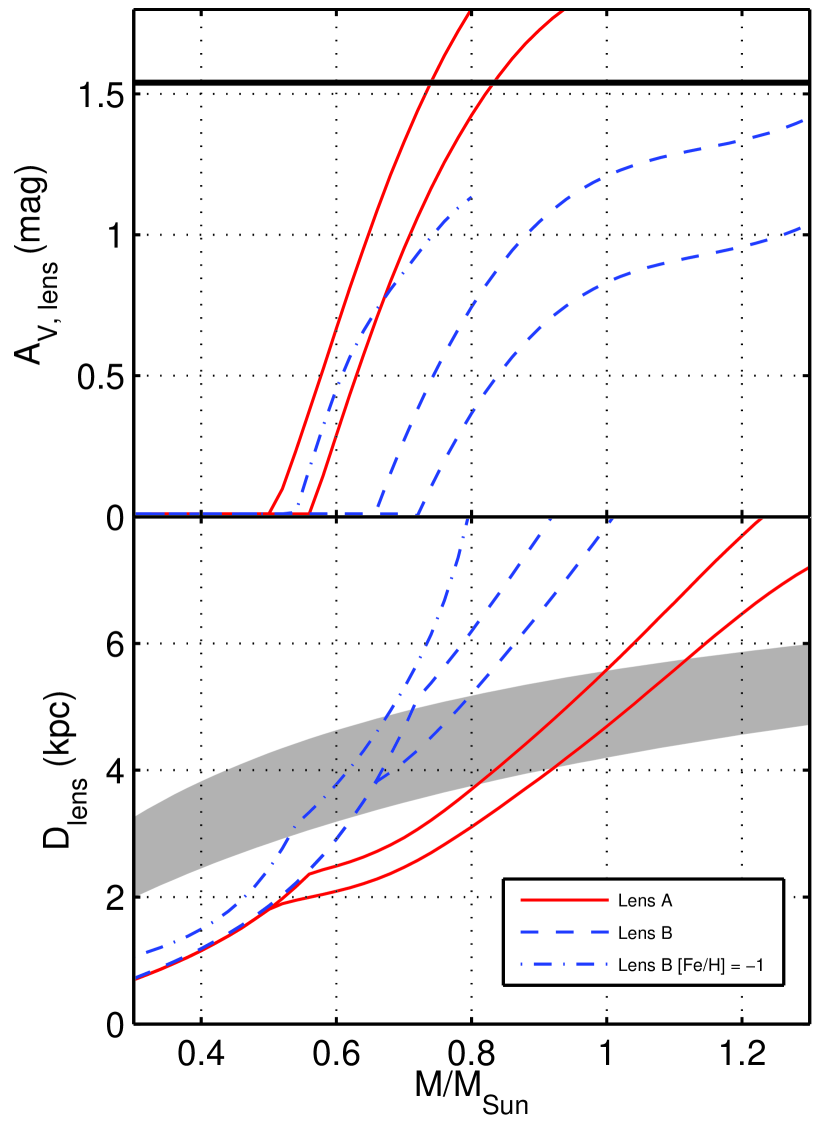
Figure 4.— Photometric solutions for the lens distance and required extinction (top panel) as a function of the lens mass are shown. The gray area covers microlensing geometries for a source at 8 kpc allowed by the measurement of the Einstein radius $\theta_{\rm E}=0.8$ mas with 20% uncertainty. For each main-sequence model we show a pair of lines that reflects the $\pm 0.1$ mag uncertainty in stellar colors. A metal-poor model is also shown for star B (dot-dashed line). The top panel shows the required extinction to match the observed magnitude and color of the lens (§5.3); the thick horizontal line marks the total Galactic extinction ($A_{\rm V}=1.54$ mag) for the line of sight from Sumi (2004).

The constraints on the lens resulting from the two major scenarios are plotted in Figure 4. The red solid lines show the photometric constraints for star A being the lens and the blue dashed lines are for star B being the lens. Each pair of lines corresponds to a range of solutions allowed by the $\pm 0.1$ mag uncertainty in stellar colors. The gray area is the geometric constraint based on the measurement of $\theta_{\rm E}$ (eq. [3]) assuming a Galactic bulge source. It is clear that a blue lens (star B) on the main sequence generally underpredicts the amount of extinction for a given distance. If the source is in the bulge, the microlensing constraint selects $D_{\rm l}$=4–5 kpc, where the blue color of the lens does not allow any significant extinction. Moving the source to a distance much larger than $D_{\rm s}=8$ kpc shifts the range of $D_{\rm l}$ upward by a few kpc, but the problem with $A_{\rm V}$ remains. The blue dot-dashed line illustrates the effect of lowering the metallicity of star B to [Fe/H] = $-$1.0. This does solve the issue of extinction, but requires that the lens is a metal-poor subdwarf in the Galactic halo, or perhaps in the thick disk. Such a possibility is unlikely since the halo and thick disk contribute only a small fraction of stars within the Galactic disk. The mass and the distance of the lens are then $M\sim 0.6M_{\odot}$ and $D_{\rm l}\sim 4$ kpc. The solution with a red lens (star A) is also not without a wrinkle, because in order to avoid overshooting the total extinction for the bulge we need to make $\theta_{\rm E}$ about 20% larger and the lens $\sim 0.1$ mag bluer compared to the best estimates. Nevertheless, we can still find a consistent answer within $1\sigma$ uncertainties. In this scenario the lens is a main-sequence star with $M=0.8$–$0.9M_{\odot}$ (spectral type G5–K0) at a distance of $D_{\rm l}\approx 4$ kpc.

6. Discussion

There is little doubt that we are directly observing the lens in the MACHO-95-BLG-37 event as it separates from a nearly perfect alignment with the microlensed source. However, the final identification of the gravitational lens is somewhat problematic. While the light curve models combined with the photometric data for individual objects favor a scenario with a blue lens and a red source, the opposite assignment is much more plausible in the context of the color-magnitude diagram for the line of sight and the observed proper motions. In any case, the lens is a relatively bright star with the mass of $\sim 0.6M_{\odot}$ or $\sim 0.9M_{\odot}$. It is conceivable that additional factors such as binarity of stars affect the interpretation of the MACHO-95-BLG-37 event, but a conclusive resolution of the present conflict will require new data. High quality spectroscopy would unambiguously pinpoint both the 3-D kinematics and the distance scale.

For the first time in a Galactic bulge event the lens and source have been directly resolved. This is an important addition to the sample of one consisting of the MACHO-LMC-5 event. There are thousands of known Galactic bulge microlensing events and several dozen of those have archival HST pointings suitable for follow-up proper motion work. In our proper motion mini-survey (Kozłowski et al. 2006) we included 35 of those fields, and have already identified several more promising candidate lenses. As pointed out by Han & Chang (2003) and (2006), in a few per cent of microlensing events toward the Galactic center a lens with characteristic motion $\mu_{\rm rel}\lesssim 10{\rm{\rm\,mas}}\,{\rm yr}^{-1}$ may be detectable a decade after the microlensing episode. We are only beginning to probe directly the mass spectrum of the Galactic microlenses; however, we can expect that in the short term the progress will accelerate considerably due to availability of the archival and future HST pointings.

References

- Abe et al. (2003) Abe, F. et al. 2003, A&A, 411, L493
- Alard & Lupton (1998) Alard, C., Lupton, R. H. 1998, ApJ, 503, 325
- Alard (2000) Alard, C. 2000, A&AS, 144, 363
- Alcock et al. (1996) Alcock, C. et al. 1996, ApJ, 471, 774
- Alcock et al. (1998) Alcock, C., et al. 1998, ApJ, 499, L9
- Alcock et al. (2001) Alcock, C. et al. 2001, Nature, 414, 617
- Alcock et al. (2001) Alcock, C. et al. 2001, ApJ, 550, L169
- An et al. (2002) An, J. H. et al. 2002, ApJ, 572, 521
- Baraffe et al. (1997) Baraffe, I., Chabrier, G., Allard, F., Hauschildt, P. H. 1997, A&A, 327, 1054
- Beaulieu et al. (2006) Beaulieu, J.-P. et al. 2006, Nature, 439, 437
- Bennett et al. (2002) Bennett, D. P. et al. 2002, ApJ, 579, 639
- Bennett et al. (2006) Bennett, D. P., Anderson, J., Bond, I. A., Udalski, A., Gould, A. 2006, ApJ, 647, L171
- Bessell (1990) Bessell, M. S. 1990, A&AS, 83, 357
- Bond et al. (2004) Bond, I. A. et al. 2004, ApJ, 606, L155
- Chang & Refsdal (1984) Chang, K., Refsdal S. 1984, A&A, 132, 168
- Drake et al. (2004) Drake, A. J., Cook, K. H., Keller, S. C. 2004, ApJ, 607, L29
- Gould et al. (1994) Gould, A., Miralda-Escude, J., Bahcall, J. N. 1994, ApJ, 423, L105
- Gould (2004) Gould, A. 2004, ApJ, 606, 319
- Gould et al. (2004) Gould, A., Bennett, D. P., Alves, D. R. 2004, ApJ, 614, 404
- Gould et al. (2006) Gould, A. et al. 2006, ApJ, 644, L37
- Han & Chang (2003) Han, C., Chang, H.-Y. 2003, MNRAS, 338, 637
- Ibata et al. (1997) Ibata, R. A., Wyse, R. F. G., Gilmore, G., Irwin, M. J., Suntzeff, N. B. 1997, AJ, 113, 634
- Jiang et al. (2004) Jiang, G. et al. 2004, ApJ, 617, 1307
- Kozłowski et al. (2006) Kozłowski, S., Woźniak, P. R., Mao, S., Smith, M. C., Sumi, T., Vestrand, W. T., Wyrzykowski, Ł. 2006, MNRAS, 370, 435
- Krist (1993) Krist, J. 1993, ASPC, 52, 536
- Krist (1995) Krist, J. 1995, ASPC, 77, 349
- Mao (1992) Mao, S. 1992, ApJ, 389, 63
- Paczyński (1996) Paczyński, B. 1996, ARA&A, 34, 419
- Perryman et al. (1997) Perryman, M. A. C. et al. 1997, A&A, 323, L49
- Popowski et al. (2005) Popowski, P. et al. 2005, ApJ, 631, 879
- Reid (1991) Reid, N. 1991, AJ, 102, 1428
- Schechter et al. (1993) Schechter P. L., Mateo, M., Saha, A. 1993, PASP, 105, 1342
- Schmidt-Kaler (1982) Schmidt-Kaler, T. 1982, in Allen’s Astrophysical Quantities, ed. A. N. Cox (New York: Springer), 388
- Sumi (2004) Sumi T. 2004, MNRAS, 349, 193
- Thomas et al. (2005) Thomas, C. L. et al. 2005, ApJ, 631, 906
- Udalski (2000) Udalski, A. 2000, ApJ, 531, L25
- Udalski et al. (2002) Udalski, A. 2002, Acta Astronomica, 52, 217
- Udalski et al. (2005) Udalski, A. et al. 2005, ApJ, 628, L109
- Woźniak (2000) Woźniak, P. 2000, Acta Astronomica, 50, 421
- (40) Wood, A. 2006, unpublished PhD thesis (Univ. of Manchester)