Chandra and XMM-Newton Detection of Large-scale Diffuse X-ray Emission from the Sombrero Galaxy

Abstract

We present an X-ray study of the massive edge-on Sa galaxy, Sombrero (M 104; NGC 4594), based on XMM-Newton and Chandra observations. A list of 62 XMM-Newton and 175 Chandra discrete X-ray sources is provided, the majority of which are associated with the galaxy. Spectral analysis is carried out for relatively bright individual sources and for an accumulated source spectrum. At energies $\gtrsim 2$ keV, the source-subtracted X-ray emission is distributed similarly as the stellar K-band light and is primarily due to the residual emission from discrete sources. At lower energies, however, a substantial fraction of the source-subtracted emission arises from diffuse hot gas extending to $\sim 20$ kpc from the galactic center. The galactic disk shows little X-ray emission and instead shadows part of the X-ray radiation from the bulge. The observed diffuse X-ray emission from the galaxy shows a steep spectrum that can be characterized by an optically-thin thermal plasma with temperatures of $\sim$ 0.6-0.7 keV, varying little with radius. The diffuse emission has a total luminosity of $\sim 3\times 10^{39}{\rm~{}erg~{}s^{-1}}$ in the 0.2-2 keV energy range. This luminosity is significantly smaller than the prediction by current numerical simulations for galaxies as massive as Sombrero. However, such simulations do not include the effect of quienscent stellar feedback (e.g., ejecta from evolving stars and Type Ia supernovae) against the accretion from intergalactic medium. We argue that the stellar feedback likely plays an essential role in regulating the physical properties of hot gas. Indeed, the observed diffuse X-ray luminosity of Sombrero accounts for at most a few percent of the expected mechanical energy input from Type Ia supernovae. The inferred gas mass and metal content are also substantially less than those expected from stellar ejecta. We speculate that a galactic bulge wind, powered primarily by Type Ia supernovae, has removed much of the “missing” energy and metal-enriched gas from the region revealed by the X-ray observations.

1 Introduction

Galactic bulges are an important component of early-type spiral galaxies. X-ray studies of the high-energy phenomena and processes in galactic bulges provide a vital insight into our understanding of galaxy formation and evolution. Several facts make Sombrero (Table 6) an ideal target for such a study: 1) This nearby Sa galaxy is massive (circular rotation speed of $\sim 370{\rm~{}km~{}s^{-1}}$) and bulge-dominated, and hence a potential site for probing a large amount of hot gas from intergalactic accretion (e.g., Toft et al. 2002) and/or internal stellar feedback (e.g., Sato & Tawara 1999); 2) The high inclination of the galaxy (84^∘) allows for a clean separation between the disk and bulge/halo components; 3) A well-determined distance ($8.9\pm 0.6$ Mpc) of the galaxy minimizes the uncertainty in the measurement of X-ray luminosities; 4) As indicated by its very low specific far-infrared and diffuse radio fluxes (Bajaja et al. 1988), the galaxy shows little indication for recent star formation, minimizing the possibility of heating and/or gas ejection from the galactic disk; 5) The galaxy is isolated and thus uncertainties resulting from galaxy interaction are miminal. Therefore, Sombrero is particularly well-suited for an X-ray study of high-energy stellar and interstellar products in a galactic bulge and their relationship to the galactic disk and to the intergalactic environment.

Existing X-ray studies of Sombrero have focused on its discrete X-ray sources. Di Stefano et al. (2003) reported the detection of 122 X-ray sources, based on a Chandra ACIS-S observation of the galaxy. In particular, they classified a population of very soft X-ray sources, which tend to concentrate in the core region of the galactic bulge. Wang (2004) conducted a careful analysis of the luminosity function of the discrete X-ray sources detected from the same observation by correcting for incompleteness and Eddington bias in the source detection and by removing statistical interlopers in the field. The X-ray behavior of the central AGN has been studied by Pellegrini et al. (2003), based on an XMM-Newton observation as well as the Chandra data.

We here report a systematic analysis of the XMM-Newton and Chandra observations (Figs. 1 and 2), focusing on the study of diffuse X-ray emission in Sombrero. The Chandra data, with superb spatial resolution, are well-suited for the study of the galaxy’s inner region where the X-ray source density is high. However, the field of view (FoV) of the Chandra ACIS-S, especially that of the S3 chip ($\sim 8^{\prime}\times 8^{\prime}$), does not provide a full coverage of the large-scale X-ray emission of the galaxy (cf. Fig. 3). The XMM-Newton EPIC observation, on the other hand, has a substantially larger FoV, allowing us to probe the extent of the global diffuse X-ray emission. The combination of the two observations thus provides us with the most comprehensive X-ray view of the galaxy.

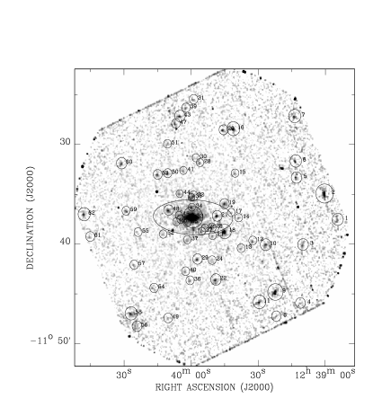
Figure 1: EPIC-PN intensity image of the M 104 field in the 0.5-7.5 keV band after a flat-fielding. An adaptively smoothed background has been subtracted from the image to highlight discrete sources which are outlined with circles for source-removal (see § 4.1). The source numbers (Table 3) are also marked. The ellipse ($8\farcm 7{\times}3\farcm 5$) illustrates the optical $I_{B}=25{\rm~{}mag~{}arcsec^{-2}}$ isophote of the galaxy.

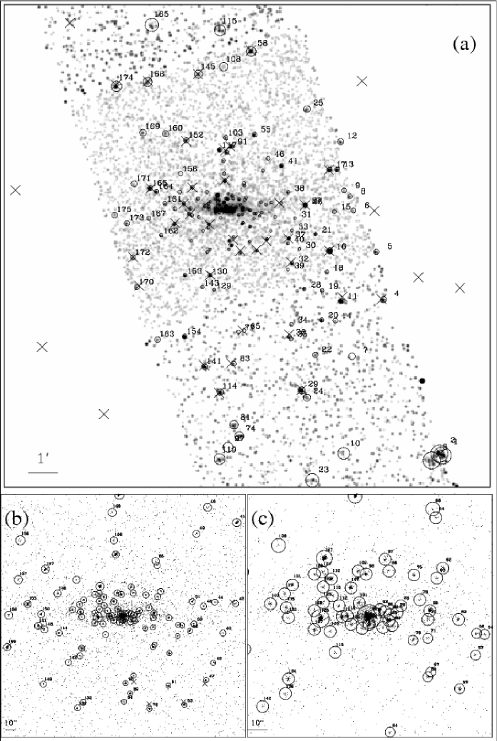
Figure 2: ACIS-S 0.3-7 keV band intensity images: (a) the whole source detection field, over which the image is smoothed with a Gaussian of FWHM equal to 3$\farcs$9; (b) the inner $\sim 4^{\prime}{\times}4^{\prime}$ region around the center of M 104; (c) the very central $\sim 2^{\prime}{\times}2^{\prime}$ region around the galactic center. Detected X-ray sources (Table 2) are outlined with circles for source-removal (see § 4.1). Positions of sources detected by the EPIC-PN are marked with crosses.

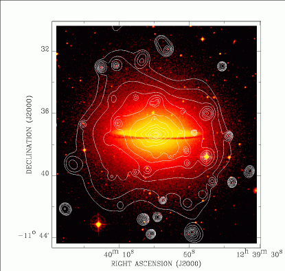
Figure 3: EPIC-PN 0.5-2 keV intensity contours overlaid on the digitized sky-survey blue image of M 104. The X-ray intensity is adaptively smoothed with the CIAO csmooth routine with a signal-to-noise ratio of $\sim 3$. The contours are at (1.4, 1.8, 2.6, 4.2, 7.4, 13.8, 27, 52, 103, 206, 411, 820, and 1640)$\times 10^{-3}{\rm~{}cts~{}s^{-1}~{}arcmin^{-2}}$ above a local background level of 2.0$\times 10^{-3}{\rm~{}cts~{}s^{-1}~{}arcmin^{-2}}$.

2 Observations and Data Reduction

Our data calibration procedures have been detailed in previous works which dealt with similar Chandra and XMM-Newton observations (e.g., Wang et al. 2003; Li et al. 2006). Here we summarize the essential aspects that are specific to the current data.

2.1 Chandra observations

The Chandra ACIS-S observation of Sombrero (Obs. ID. 1586) was taken on May 31, 2001, with an exposure of 18.8 ks. Our work uses the data primarily from the on-axis S3 chip, although part of the adjacent FI chips (S2 and S4) are also included in the source detection. We reprocessed the Chandra data, using CIAO, version 3.2.1 and the latest calibration files. We also removed time intervals with significant background flares, i.e., those with count rates $\gtrsim 3\sigma$ and/or a factor of $\gtrsim 1.2$ off the mean background level of the observation. This cleaning resulted in an effective exposure of 16.4 ks for subsequent analysis. We created count and exposure maps in the 0.3-0.7, 0.7-1.5, 1.5-3, and 3-7 keV bands. Corresponding background maps were created from the “stowed background” data, which contain only events induced by the instrumental background. A normalization factor of $\sim 1.05$ was applied to the exposure of this “stowed background” data in order to match its 10-12 keV count rate with that of Obs. 1586.

2.2 XMM-Newton observations

The XMM-Newton EPIC observation of Sombrero (Obs. ID 0084030101) was taken on December 28, 2001, with the thin filter and with a total exposure of 43 ks. We calibrated the data using SAS, version 6.1.0, together with the latest calibration files. In this work, we only use the EPIC-PN data. We found that a large fraction of the observation was strongly contaminated by cosmic-ray-induced flares. To exclude these flares, we removed time intervals with count rates greater than 11 ${\rm cts~{}s^{-1}}$ in the 0.2-15 keV band, about a factor of 1.2 above the quiescent background level, and some additional intervals with residual flares found in sub-bands. The remaining exposure is only 10.8 ks for the PN. We then constructed count and exposure maps in the 0.5-1, 1-2, 2-4.5, and 4.5-7.5 keV bands for flat-fielding. We also created corresponding background maps from the “filter wheel closed” (FWC) data , chiefly for instrumental X-ray background subtraction. However, we found that at energies above 5 keV the spectral shape of the instrumental background of Obs. 0084030101 is apparently different from that of the FWC data, making a simple normalization inapplicable. Therefore, the FWC data are only used in producing large-scale images. Background adoption for spectral analysis will be further discussed in § 4.2.

3 Discrete X-ray sources

Fig. 3 shows the overall 0.5-2 keV X-ray intensity image of Sombrero obtained from the PN. The morphology appears more-or-less symmetric, reminiscent of the optical light distribution of the galaxy. The X-ray emission likely represents a combined contribution from discrete sources and truly diffuse hot gas. We first detect individual sources and characterize their properties. Then we try to isolate and study the diffuse X-ray component in § 4.

3.1 Source dection and astrometry correction

We detect 175 Chandra and 62 XMM-Newton discrete X-ray sources. Tables 2 and 3 summarize the detection results. The source detection is carried out for each observation in the broad (B), soft (S), and hard (H) bands, defined differently for the ACIS-S and PN data, as noted in the tables. Following the procedure detailed in Wang (2004), we use a combination of source detection algorithms: wavelet, sliding-box, and maximum likelihood centroid fitting. The map detection and the maximum likelihood analysis are based on data within the 50% PSF energy-encircled radius (EER) for the PN and the 90% EER for the ACIS-S. The accepted sources all have a local false detection probability $P\leq 10^{-6}$. For ease of reference, we will refer to X-ray sources detected in the PN and the ACIS-S with prefixes XP and XA, respectively (e.g., XP-13).

Although the pointing uncertainty of Chandra is on average less than $\sim 1$${}^{\prime\prime}~{}$, it is still desirable to quantify and possibly improve the astrometric accuracy of any particular observation. We first use the Two Micron All Sky Survey (2MASS) All-Sky Catalog of Point Sources (Cutri et al. 2003) to find potential near-IR counterparts for an astrometric calibration. The astrometry of the 2MASS objects is generally much better ($\sim 0\farcs 1$). We cross-correlate the spatial positions of the objects in the catalog with those of the X-ray sources listed in Tables 2 and 3. For each ACIS-S source, we use a matching radius of twice its position uncertainty, with lower and upper limits of 1${}^{\prime\prime}~{}$and 2${}^{\prime\prime}~{}$. The lower limit is set to account for any systematic errors in the X-ray source positions, whereas the upper limit is to minimize the probability of chance coincidence. Similar calibration is also done for the PN sources outside the ACIS-S FoV (Fig. 2), with lower and upper matching radii of 2${}^{\prime\prime}~{}$and 4${}^{\prime\prime}~{}$.

The calibration gives five Chandra/2MASS position coincidences. We estimate the required astrometric correction to be 0$\farcs$4 to the west and 0$\farcs$5 to the north, based on a $\chi^{2}$ fit to the R.A. and DEC. offsets of the five matched Chandra/2MASS pairs. The correction is insensitive (with changes $\lesssim 0\farcs 1$) to the exclusion of any one of the entries in the fit. The correction improves the $\chi^{2}/d.o.f.$ from 21/10 to 4/8. After correcting for the X-ray astrometry, one additional position coincidence (XA-149) is found.

Table 4 presents the matching results, including the position offset of each match, together with the expected position uncertainties quoted from Tables 1 and 2; there is no match with multiple 2MASS objects. The table also includes the J, H, and K_s magnitudes of the matched 2MASS objects; the $3\sigma$ limiting sensitivities of the catalog are 17.1, 16.4 and 15.3 mag in the three bands. We estimate the expected number of chance projections of 2MASS objects within the matching regions to be $\sim 0.2$ for the ACIS-S sources and 0.5 for the PN sources, based on the surface number density of 2MASS objects within annuli of 4${}^{\prime\prime}~{}$-15${}^{\prime\prime}~{}$radii around the X-ray sources. Therefore, it is possible that a couple of the matches may just be such chance projections.

The source locations are marked in Figs. 1 and 2. Essentially all PN sources within the field of Fig. 2a are also detected in the ACIS-S data. All relatively bright ACIS-S sources, except for those in the nuclear region, are detected in the PN data. These consistencies indicate no strong variability of the sources between the two observations. Source confusion is serious for the PN data, because of the limited spatial resolution. Some of the PN detections represent combinations of multiple discrete sources, e.g., XP-42 is a combination of XA-148 and 151. This is particular the case in the nuclear region (Fig. 2c).

We note that the source detection limit is significantly higher in the PN data than in the ACIS-S data. The majority of detected sources are of two populations: sources associated with the galaxy and extragalactic sources mostly being background AGNs. Applying the luminosity function (LF) of the AGNs obtained by Moretti et al. (2003), we estimate the number of detected AGNs to be 15.5 (2.3) in the ACIS-S (PN) FoV.

3.2 Individual spectra of bright sources

There are eight bright sources in the ACIS-S field as deteceted with a count rate higher than 0.01 ${\rm~{}cts~{}s^{-1}}$. These are XA-10, 15, 26, 28, 96, 98, 121 and 124 (Table 2). Among them, XA-15 is a foreground star; XA-10 and XA-28 are located outside the S3 chip; X-96 is the nucleus which have been studied by Pellegrini et al. (2003); X-98 is located within 3^′′ from the nucleus. We perform spectral fit to individual ACIS-S spectra of the rest three sources, each extracted from a circular region of twice the 90% EER. Corresponding background spectra are extracted from the source-free vicinity of each source. The spectra of XA-26 and XA-121 are fitted by an absorbed power-law, whereas the spctrum of XA-124, being very soft, is fitted by an absorbed blackbody. The fit results, summerized in Table 5, are statistically consistent with those obtained by Di Stefano et al. (2003). The spectra and the best-fit models are shown in Fig. 4a-4c.

Figure 4: ACIS-S spectra of discrete sources in the field of M 104 : (a)-(c) individual spectra of three bright sources; (d) an accumulated spectrum of sources within the D₂₅ ellipse. Best-fit models to the spectra are also shown. The lower panels show the data-to-model ratios.

3.3 Accumulated source spectrum

We further obtain an accumulated ACIS-S spectrum of the sources to characterize their average spectral property (Fig. 4d). The spectrum is extracted from sources within the $I_{B}=25{\rm~{}mag~{}arcsec^{-2}}$ isophote ($D_{25}$ ellipse; 8$\farcm$7$\times$3$\farcm$5), except for the nuclear source and the three bright sources discussed above. The total number of included sources is $\sim$110. For each source, a circular region of twice the 90% EER is adopted for accumulating the spectrum. A background spectrum is extracted from the rest region of the ellipse. In the PN data, only ten sources are detected within the $D_{25}$ ellipse and four of them are located within 1$\farcm$5 from the galactic center, where the emission of the nucleus largely affects. Therefore, we do not analyze an accumulated source spectrum from the PN.

We use an absorbed power-law model to fit the accumulated spectrum, with the absorption being at least that supplied by the Galactic foreground. The model offers an acceptable fit to the spectrum (Table 5), giving a best-fit photon index of $1.51^{+0.10}_{-0.09}$ and a 0.3-7 keV intrinsic luminosity of $\sim 2.6{\times}10^{40}{\rm~{}ergs~{}s^{-1}}$. All quoted errors in this paper are at the 90% confidence level. The slope of the power-law is typical for composite X-ray spectra of low-mass X-ray binaries observed in nearby galaxies (LMXBs; e.g., Irwin, Athey & Bregman 2003). We note that none of the included sources contributes more than 5% of the total counts to the accummulated spectrum. Therefore, the spectrum, along with the fitting model, can be used to characterize the average spectral property of sources.

4 The source-subtracted X-ray emission

Our main interest here is in the diffuse X-ray emission from Sombrero. A first step towards isolating the diffuse emission is to subtract the detected discrete sources from the images. To do so, we exclude regions enclosing twice the 50% (90%) EER around each PN (ACIS-S) source with a count rate ($CR$) $\lesssim 0.01{\rm~{}cts~{}s^{-1}}$. For brighter sources, a factor of $1+{\rm log}(CR/0.01)$ is further multiplied to the source-subtraction radius. Our choice of the regions is a compromise between excluding a bulk of the source contribution and preserving a sufficient field for the study of the source-subtracted emission. With the above criteria about $80\%$ ($95\%$) of photons from individual sources are removed from the PN (ACIS-S) image.

The source-subtracted emission presumably consists of two components: the emission of truly diffuse gas and the collective discrete contributions from the residual emission of detected sources and the emission of undetected sources below our detection limit. In practice, the discrete component can be constrained from its distinct spatial distribution and spectral property. Below we isolate the two components and characterize the properties of the diffuse emission.

4.1 Spatial properties

4.1.1 Surface intensity profiles

We construct instrumental background-subtracted and exposure-corrected galactocentric radial surface intensity profiles for the source-subtracted emission, in the soft (0.5-1 keV for the PN; 0.3-0.7 keV for the ACIS-S), intermediate (1-2 keV for the PN; 0.7-1.5 keV for the ACIS-S) and hard (2-7.5 keV for the PN; 1.5-7.0 keV for the ACIS-S) bands (Fig. 5). While the ACIS-S instrumental background is determined from the “stowed background” data, the instrumental background rates in the PN bands are predicted from the spectral fit to a local PN background spectrum (see § 4.2). Spatial binning of annuli is adaptively adjusted to achieve a signal-to-noise ratio better than 3, with a minimum step size of 6^′′ for the PN and 3^′′ for the ACIS-S. For the PN profiles, the central 1$\farcm$5 is heavily contaminated by the emission from the nucleus. Thus our analysis for the PN data is restricted to radii beyond 1$\farcm$5. The ACIS-S data, while being capable to probe the central region, are limited by its FoV. Therefore we restrict our analysis of the ACIS-S profiles within 3$\farcm$5, a maximal radius where complete annuli can be extracted.

It is known that Sombrero has a prominent dust lane (e.g., Knapen et al. 1991; cf. Fig. 3), which may significantly absorb soft X-rays from the galaxy and hence introduce a bias to the bin-averaged intensity. Therefore when constructing the intensity profiles we exclude a region encompassing the dust lane. We use the digitized sky-survey blue image of the galaxy to map such a region of extinction, in which a pixel is adopted as the region bounary if it is dimmed by a factor $\geq$1.5 compared to the adjacent bright pixel. Visual inspection on the ACIS-S image indicates that our adopted region is coincident with a region of few registered soft X-ray photons.

To constrain the discrete component, we assume that its spatial distribution follows the near-IR light of the galaxy, which can be determined from the 2MASS K-band map (Jarrett et al. 2003). We first exclude from the map bright foreground stars and circular regions used for subtracting the discrete X-ray sources. The K-band radial intensity profile is then produced in the same manner as for the X-ray profiles. It is reasonable to assume that the discrete component dominates the X-ray emission in the hard band. Thus we use the K-band profile to fit the X-ray hard band profiles, constructed from the PN and ACIS-S data. The fitting parameters are the X-ray-to-K-band intensity ratio of the underlying stellar content ($I_{s}$) and a constant intensity ($I_{b}$) to account for the local cosmic X-ray background. We find that the X-ray hard band profiles can be well characterized by the K-band profile (Fig. 5; Table 6).

We further assume that the discrete component has a collective spectral property same as that modeled for the detected sources (§ 3.3). This allows us to use the hard band intensity to constrain the discrete component in the soft and intermediate bands. The diffuse component is then determined for these two bands by subtracting the discrete component from the total intensity profile. We then fit the radial distribution of the diffuse component with a de Vaucouleur’s law:

$$I(R)=I_{g}~{}e^{-7.67(R/r_{e})^{1/4}},$$ (1)

where $R$ is the projected galactocentric radius, $r_{e}$ the half-light radius and $I_{g}$ the central surface intensity. A paramter $I_{b}$ is also included to account for the local cosmic X-ray background. Due to the partial coverage of the overall distribution by each profile, we require in the fit that the half-light radii be identical for all profiles. We find that this characterization offers good fits to the profiles (Fig. 5; Table 6). The best-fit half-light radius is 2$\farcm$6${}^{+1\farcm 4}_{-0\farcm 9}$. In comparison, the K-band half-light radius is $\sim$ 1^′ ($\sim$ 2.6 kpc; Jarrett et al. 2003). This suggests that the distribution of hot gas is substantially more extented than that of the stellar content.

Figure 5: Radial surface intensity profiles of the instrumental background- and detected source-subtracted emission from M 104. Top: ACIS-S profiles in the 0.3-0.7 keV (left), 0.7-1.5 keV (middle) and 1.5-7 keV (right) bands. Bottom: PN profiles in the 0.5-1 keV (left), 1-2 keV (middle) and 2-7.5 (right) bands. The solid curves present model characterizations: a normalized K-band radial profile for emission from discrete sources (dotted curves), a de Vaucouleur’s law (dashed curves) for emission from diffuse hot gas, and a local constant cosmic background. See text for details.

We also construct vertical intensity profiles of the source-subtracted emission along the galaxy’s minor axis for the ACIS-S 0.3-0.7, 0.7-1.5 and 1.5-7 keV bands (Fig.6). In general, the intensity decreases rapidly with the off-disk distance. We follow the above procedure to decompose the diffuse and discrete components of the vertical profiles. An expotential law, i.e., $I(z)=I_{g}~{}e^{-|z|/z_{0}}$, is used to fit to the vertical distribution of the diffuse component. The scale height $z_{0}$ is allowed to be different between the south and north sides of the midplane. The fit is marginally accetable, with excess existing at $\sim 2^{\prime}$ from the midplane on both sides. Fit results (Table 7) show that in each band there is no significant asymmetry in the intensity distribution with respect to the midplane. The best-fit scale height in the soft band ($\sim$ 1/4 arcmin) is less than that in the intermediate band ($\sim$ 1/3 arcmin), indicating that emission is softer in the central region than in the extraplanar region. When the above fit is restricted to a vertical distance $\geq$ 0$\farcm$5, the best-fit scale heights for the soft and intermediate bands are nearly identical ($\sim 1^{\prime}$). This is evident that the temperature of hot gas around the disk plane is lower than that in the bulge.

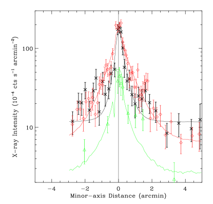
Figure 6: ACIS-S intensity distribution along the direction perpendicular to the disk of M 104, in the 0.3-0.7 keV (black crosses), 0.7-1.5 keV (red diamonds), and 1.5-7 keV (green triangles) bands. The full width along the direction parallel to the major axis used for averaging the intensity is 4^′ ($\sim$10 kpc). The adaptive steps along the minor axis achieve a signal-to-noise ratio greater than 3, with a minimum of stepsize of 6^′′. The vertical line represents the position of the major axis of the disk, whereas the horizontal axis marks the vertical distance along the minor axis (south as negative).

4.1.2 Inner region and substructures

We use the ACIS data to probe the diffuse X-ray properties in the inner region of the galaxy. We fill the holes from the source removal with the values interpolated from surrounding bins. Fig. 7 shows “diffuse” X-ray intensity contours, which are substantially less smoothed than presented in Fig. 3. There are considerable substructures in the inner region. Inner contours are extended more to the north than to the south (where strong intensity gradients are found), indicating a heavier absorption of X-ray emission to the south. This is clearly due to the prominent dust lane that lies at the 10${}^{\prime\prime}~{}$-25${}^{\prime\prime}~{}$ range to the south of the major axis (Knapen et al. 1991). The intensity contours also become strongly elongated along the galactic disk.

Fig. 7 also presents in grey scale a continuum-subtracted H$\alpha$ image of Sombrero, obtained with the 0.9 meter telescope at Kitt Peak National Observatory in 1999. The details of observations are presented elsewhere (Hameed & Devereux 2005). H$\alpha$ emission is distributed, primarily, in an annulus, and individual HII regions can be identified on the ring. There is some H$\alpha$ emission within the ring, but it is difficult to tell from the image if the emission is diffuse or if it contains HII regions. The H$\alpha$ ring follows the optical dust lane but is located on its inner side. High extinction possibly obscures ionized emission from the dust lane itself.

Total H$\alpha$ flux for Sombrero, uncorrected for internal or external extinction, is calculated to be $\sim 0.8\times 10^{-12}{\rm~{}ergs~{}s^{-1}~{}cm^{-2}}$, which translates to a luminosity of $\sim 7.6\times$ 10${}^{39}{\rm~{}ergs~{}s^{-1}}$. Using Kennicutt’s (1998) formula, we derive a star formation rate of $\sim 0.1{\rm~{}M_{\odot}~{}yr^{-1}}$, which is lower than the average star formation rate (0.9 ${\rm~{}M_{\odot}~{}yr^{-1}}$) for early-type spirals (Hameed & Devereux 2005).

Fig. 7 shows that X-ray intensity drops abruptly in the field covered by the front side of the H$\alpha$ disk, corresponding to the inner region of the cold gas disk of the galaxy. This means that the H$\alpha$-emitting region does not contribute appreciable amounts to X-ray radiation. In contrast, good H$\alpha$/X-ray correlation is typically seen in late-type spirals (e.g., Strickland et al. 2004; Wang et al. 2003). In fact, the diffuse X-ray intensity in Sombrero is so low in the field covered by the front side of the cool gas disk that the disk must be absorbinga large fraction of X-ray emission from the region beyond.

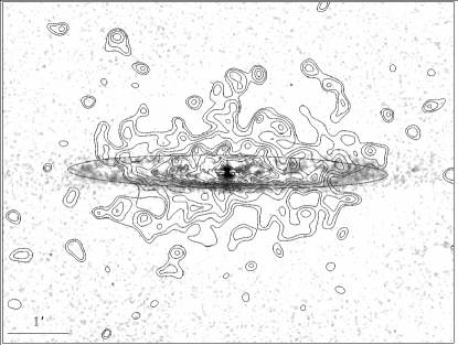
Figure 7: ACIS-S 0.3-1.5 keV intensity contours overlaid on the continuum-subtracted H$\alpha$ image of M 104. The X-ray intensity is smoothed adaptively with a count-to-noise ratio of 4 after source-subtraction.

We probe the azimuthal variation of diffuse emission in the inner region. Fig. 8 shows the azimuthal ACIS-S 0.3-1.5 keV intensity distributions. The distributions deviate from axisymmetry significantly. But the deviations are largely coupled with the orientation of the bulge (0^∘ aligns with the minor axis). When the azimuthal intensity distributions are measured within elliptical annuli with an axis ratio similar to that of the bulge (Fig. 8), the deviations are significantly reduced, with smaller scale fluctuations remaining in certain azimuthal ranges, especially in the inner region. For example, dips present at $\sim 200^{\circ}-250^{\circ}$ and $\sim 330^{\circ}-350^{\circ}$ find their counterparts in Fig. 7. At larger radii, only moderate deviations from axisymmetry can be seen from the azimuthal intensity distributions for the PN data. When an axis ratio of 0.8 is adopted to reflect the geomoetry of the bulge, most of the deviations vanish and no substantial fluctuations are present. This is evidence that the diffuse emission is nearly axisymmetric at large scale.

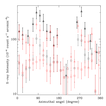
Figure 8: Azimuthal diffuse intensity distributions in the ACIS-S 0.3-1.5 keV band, averaged within annuli with inner-to-outer radii of 30^′′-1^′ (black triangles) and 1^′-2^′ (black squares). As comparison are similar distributions (red triangles and squares) within elliptical annuli of an axis ratio of 2/3. The angle is counterclockwise from the minor axis (north). Contribution from unresolved sources is subtracted according to the underlying K-band light (§ 4.1; Table 6). Adaptive binning is taken to have a minimum step of 15^∘ and to achieve a signal-to-noise ratio better than 3.

4.2 Spectral properties of the diffuse X-ray emission

With the above spatial properties in mind, we perform spectral analysis of source-subtracted emission from a series of concentric annuli around the galactic center. Specifically, spectra are extracted from two annuli with inner-to-outer radii of 30^′′-1^′ and 1^′-2^′ for the ACIS-S data and two annuli of 2^′-4^′ and 4^′-6^′ for the PN data. The dust lane region (§ 4.1.1) is excluded from the spectral extraction.

Two factors complicate the background determination in our spectral analysis. First, the sky location of Sombrero is on the edge of the North Polar Spur (NPS), a Galactic soft X-ray-emitting feature (Snowden et al. 1995). The NPS introduces an enhancement to the local background, particularly at low energies. Secondly, the X-ray emission from Sombrero extends to at least 6^′ from the galactic center (§ 4.1.1). Thus a local background cannot be extracted for the ACIS-S data. While the PN FoV still allows for a local background, the vignetting effect at large off-axis angles needs to be properly corrected for in the background subtraction. Generally, this can be achieved with the “double-subtraction” procedure: a first subtraction of the non-vignetted instrumental background followed by a second subtraction of the vignetted local cosmic background. Such a procedure relies on the assumption that the template instrumental background can effectively mimic that of a particular observation.

We intend to perform the “double-subtraction” procedure to determine the background. First we extract the PN background spectrum from a source-subtracted annulus with inner-to-outer galactocentric radii of 8^′-11^′, a region containing little emission from the galaxy (Fig. 5). However, at energies $\geq$ 5 keV, where the instrumental background is predominant, the local background spectrum is found to be significantly harder than the spectrum extracted from the FWC data. Therefore, we decide to characterize the local background spectrum of PN, both instrumental and cosmic, by a combination of plausible components. To model the instrumental background, a broken power-law plus several Gaussian lines is applied (Nevalainene, Markevitch & Lumb 2005). The modeling of the cosmic background consists of three components. Two of them are thermal (the APEC model in XSPEC), representing the emission from the Galactic halo (temperature $\sim$ 0.1 keV) and the NPS (temperature $\sim$ 0.25 keV; Willingale et al. 2003), respectively. The third component is a power-law with the photon index fixed at 1.4, representing the unresolved extragalactic X-ray emission (Moretti et al. 2003). Our combined model results in a good fit to the local background spectrum. We note that the decomposition of the local background is not unique, especially at lower energies ($\lesssim$ 1 kev). We verify our modeling by the fact that the fitted parameters of these commonly used cosmic components are in good agreement with independent measurements (e.g., Willingale et al. 2003; Moretti et al. 2003). The background spectrum in the 0.5-7 keV range, grouped to have a minimum number of 30 counts in each bin, is shown in Fig.9. The model, scaled according to the corresponding sky areas, is included in the following fit to the PN spectra of source-subtracted emission.

Figure 9: The PN background spectrum with the best-fit model. Note for a strong instrumental line at the energy of $\sim$ 1.5 keV. See text for details.

The spectral shape of the ACIS-S instrumental background is rather stable at energies $\geq$ 0.5 keV. Also, as the ACIS-S spectra of source-subtracted emission are extracted within the central 2^′ where the surface intensity is peaked, a small uncertainty in the instrumental bakcground subtraction would only cause a minor effect in the analysis. Therefore, we directly subtract a “stowed backgroud” spectrum from the ACIS-S spectra of source-subtracted emission and group them to achieve a signal-to-noise ratio better than 3. The remaining cosmic X-ray background are modeled with the same components as for the PN spectra. We note that an additional factor of 0.43, estimated from the LF obtained by Moretti et al. (2003), is multiplied to the scaling of the extragalactic component in order to account for the lower source detection limit in the ACIS-S data (Wang 2004).

The spectra show a clear line feature at $\sim$0.9 keV (Fig. 10), presumably due to the Fe L-shell complex contributed by the hot gas, while at energies above 1.5 keV the spectra are dominated by the residual emission of discrete sources. We account for the discrete contribution with a power-law model (PL) with a fixed photon index of 1.51 (Table 5), again assuming that its collective spectral shape is same as that of the detected sources. This PL, combined with a thermal plasma emission model (APEC) characterizing the emission of hot gas, is used to simultaneously fit the four spectra. Both components are subject to the Galactic foreground absorption. The temperature of the hot gas is allowed to vary, but the abundance is linked among the four spectra. We adopt the abundance standard of Grevesse and Sauval (1998) and set a physically meaningful upper limit of 10 solar for the abundance. The model gives a statistically acceptable fit to all four spectra, with the overall $\chi^{2}/d.o.f.$ = 481.9/511. Fit results (Table 8) suggest that the gas temperature vary little with radius. Interestingly, the metal abundance ($>$ 0.4 solar) is well distinguished from very sub-solar values that were often reported in galactic X-ray studies (e.g., NGC 253, Strickland et al. 2002; NGC 4631, Wang et al. 2001). We suggest that this owes to the proper modeling of the local background, especially at energies below 0.7 keV, where the thermal continuum from the galaxy is highly entangled with the background components. An example of this kind has also been presented by Humphrey & Buote (2006), who find near-solar iron abundances for the hot gas in most of their sample early-type galaxies.

We further use the PROJCT model in XSPEC to fit the spectra for a 2-D to 3-D deprojection, i.e., the fitting parameters are measured for consecutive spherical shells. The fit is of similar significance, with a $\chi^{2}/d.o.f.$ = 483.2/511. Fit results are listed in Table 9, again indicating a quasi-isothemal hot gas with marginally super-solar abundance in the bulge of Sombrero.

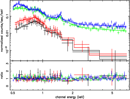
Figure 10: Spectra of the source-subtracted emission of M 104, extracted from concentric annuli of 30^′′-$1^{\prime}$ (black) and 1^′-$2^{\prime}$ (red) from the ACIS-S, and 2^′-$4^{\prime}$ (green) and 4^′-$6^{\prime}$ (Blue) from the PN. The two ACIS-S spectra are “stowed background”-subtracted. The best-fit 3-D model (see text) is also shown.

The fitted amount of the PL component in individual spectrum is verified by estimating the contribution of unresolved galactic sources. Wang (2004) obtained the LF for the detected galactic sources, mostly LMXBs. Assuming that this LF is also valid for sources below the source detection limit and varies little among the regions of our spectral interest, the contribution of unresolved sources can be taken as the integrated flux from the LF, weighted by the amount of K-band light within individual annulus. We note that the integrated flux of unresolved sources in the PN is $\sim$4 times higher than that in the ACIS-S, due to the higher source detection limit in the PN. The fitted PL fluxes (Table 9) are consistent with the above estimation to within 10% (25%) for the ACIS-S (PN) spectra. The fluxes are also consistent with the X-ray-to-K-band intensity ratio obtained from the spatial analysis (Table 6), given a count rate to flux conversion factor predicted by the PL.

Assuming a filling factor of unity, the mean densities of hot gas are $\sim$6.6, 2.8, 1.2 and 0.79 $\times 10^{-3}{\rm~{}cm^{-3}}$ in the four consecutive shells with increasing radii, derived from the 3-D spectral analysis (Table 9). These are shown versus radius in Fig. 11. Also shown is the density profile inferred from the best-fit deVaucouleur’s law to the radial intensity distributions (§ 4.1.1; Young 1976), with the assumption that the temperature of gas is constant along with radius. This profile fairly matches the spectral measurement, indicating consistency between our spatial and spectral analyses.

As shown in § 4.1.2, deviations from the assumed axisymmetry are present in the diffuse emission, especially in the inner region. Nevertheless, even in the innermost annulus, the deviations would only introduce an uncertainty of 30% in the average intensity, or $\sim$15% in the measured density. Therefore, the presence of the moderate deviations does not qualitatively affect the determination of the radial structure of hot gas and its implications as we discuss below.

The total mass of hot gas contained in the shells is $\sim$4.6 $\times 10^{8}{\rm~{}M_{\odot}~{}yr^{-1}}$, and the intrinsic 0.2-2 keV luminosity from our spectral extraction region is $\sim 3.1\times 10^{39}{\rm~{}ergs~{}s^{-1}}$. We note that these values can be approximated as the total mass and luminosity of hot gas in Sombrero, given the steep density distribution (§ 4.1.1). For example, the luminosity within the central 6^′ is about 75% of the total for a de Vaucouleur’s distribution with a half-light radius of 2$\farcm$5.

Figure 11: Crosses: the measured density of hot gas versus radius; Curves: the best-fit density profile to the radial surface intensity distribution (solid), the predicted density profiles of an adiabatic (dotted) or isothermal (dashed) gaseous corona in hydrostatic equilibrium and an 1-D steady galactic wind (dot-dashed). The profiles are assumed to be equal to the measurement at the first bin. See § 5 for details.

5 Discussion

5.1 The thermal structure of hot gas

We further compare the measured density profile with that predicted from variant thermal structures that may be assumed for the hot gas. One commonly assumed case is that the gas is in hydrostatic equilibrium, i.e., the density profile is simply determined by the gravitational potential and the equation of state for the gas. A second case is that the gas is in the form of a large-scale outflow, i.e., a galactic wind (e.g., Mathews & Baker 1971; Bregman 1980; White & Chevalier 1983), in which the physical structure of the gas is regulated by the energy and mass input from the stellar content.

We first characterize the 1-D distribution of the gravitational mass for the galactic bulge and halo. The stellar distribution in projection is assumed to follow the de Vaucouleur’s law with a half-light radius of 1^′ ($\sim 2.6{\rm~{}kpc}$; Jarrett et al. 2003). Given the K-band magnitude of Sombrero, the total stellar mass is estimated to be 1.6$\times 10^{11}{\rm~{}M_{\odot}}$, according to the K-band mass-to-light relation of Bell & de Jong (2001). However, Bridges et al. (1997) found a kinematic mass about three times of this value within a projected radius of $\sim$ 15 kpc. Therefore, a second gravitational component, i.e., dark matter, is considered. We assume that the distribution of dark matter follows the NFW profile (Navarro, Frenk & White 1996) with a scale radius of 20 kpc. This chosen scale radius is rather arbitrary but typical for a galactic dark matter halo. The mass density of the dark matter is such that the total mass (stars and dark matter) within a projected radius of 15 kpc be 5$\times 10^{11}{\rm~{}M_{\odot}}$.

For the hydrostatic equilibrium case, the density profile is calculated for two plausible states of the gas: adiabatic and an isothermal. For the galactic wind case, we have developed a simple 1-D steady dynamical model (Li & Wang in preparation). Given the above distributions of stars and dark matter, the density profile of a galactic wind is determined by the rates of total energy and mass inputs to the gas which can be estimated from empirical measurements (see § 5.3). The measured and modeled density profiles are together shown in Fig. 11, in which the modeled ones are assumed to match the measurement at the first bin. We note that there is a remarkable degeneracy between the measured density and metal abundance. Since we have assumed a single abundance independent of the radius, the overall shape of the density profile is not affected by this density-abundance degeneracy.

Fig. 11 shows that an adiabatic gas in hydrostatic equilibrium (dotted curve) is inconsistent with the measurement, whereas neither an isothermal gas in hydrostatic equilibrium (dashed curve) nor a galactic wind (dot-dashed curve) can be completely ruled out given the relatively large uncertainties in the measurement. The isothermal case is favored by the measured temperature profile with little variation, but is subject to further considerations in which stellar feedback to the hot gas is involved (see below). A galactic wind predicts a decreasing temperature with increasing radius (e.g., Chevalier & Clegg 1985) and is apparently in contradiction with the temperature measurement. However, in the galactic wind case, gas moves rapidly outward. Beyond certain radius, the recombination timescales of some species of ions may become longer than the local dynamical timescale. Recombinations of such ions occur at larger radii than the collisional ionization equilibrium (CIE) would predict. This process is called a “delayed reconbination” (e.g, Ji, Wang & Kwan 2006). Thermal processes from regions involving delayed reconbinations are of non-equilibrium ionization (NEI). Usually, when using a CIE plasma emission model (e.g., APEC) to fit an X-ray spectrum of hot gas, temperature is effectively determined by the position of line features that are prominent in the spectrum. Therefore, had the NEI emission from a galactic wind been observed, the measured temperature with a CIE model would be higher than the local gas temperature of the region being observed. Also, the emission measure would be higher than what the density distribution of the wind predicts. We suggest that this might be the case in Sombrero. A quantitative study of the NEI emission from galactic winds is under investigation.

We now turn to discuss the origin of the hot gas in specific scenarios.

5.2 Accretion from the intergalactic medium?

One scenario that may favor a quasi-hydrostatic gaseous halo comes from a specific prediction of current theories of galaxy formation and evolution: the gas is accreted from the intergalactic medium (IGM) and maintained in the halos of spiral galaxies. The IGM is supposedly heated to X-ray-emitting temperatures, chiefly due to accretion shocks and gravitational compression (e.g., Toft et al. 2002). Naturally, the X-ray luminosity of gas is a strong function of the gravitational mass of the host galaxy, as characterized by its circular rotation speed ($L_{X}\propto V_{c}^{7}$; Toft et al. 2002).

Surprisingly, there is little direct observational evidence for the presence of such X-ray-emitting halos even around massive spiral galaxies. Given the high circular rotation speed of Sombrero ($\sim 370{\rm~{}km~{}s^{-1}}$), it is a good candidate to look for X-ray signals from an accreted gaseous halo around it. Toft et al. (2002, therein Fig. 3) predict a 0.2-2 keV X-ray luminosity of $\sim 10^{41}{\rm~{}ergs~{}s^{-1}}$ for galaxies with circular rotation speeds similar to that of Sombrero, about 95% of which coming from within 20 kpc of the disk. However, the observed 0.2-2 keV diffuse X-ray luminosity from Sombrero is only $\sim 3\times 10^{39}{\rm~{}ergs~{}s^{-1}}$ within the central $\sim$ 15 kpc. Therefore, there is a remarkable discrepancy between the amount of observed extraplanar hot gas and that predicted by numerical simulations.

If the hot gas in Sombrero is indeed accreted from the IGM, what may be the cause for this discrepancy? One plausible answer is that the existing simulations have not adequately accounted for the feedback from galaxies, especially the heating due to Type Ia supernovae (SNe). Such stellar feedback tends to provide an effective form of large-scale distributed heating and thus reduce the cooling of gas in the galactic bulges and halos. If the feedback is strong enough, the galaxy may even cease further accretion.

5.3 Stellar feedback from Sombrero

Empirically, stars in a galactic bulge continuously deposit energy and mass to the interstellar medium (ISM) at rates of $\sim$$6\times 10^{40}$$[L_{B}/(10^{10}L_{B,\odot})]$ ${\rm~{}ergs~{}s^{-1}}$ and $\sim$$0.2$$[L_{B}/(10^{10}L_{B,\odot})]$ ${\rm~{}M_{\odot}~{}yr^{-1}}$ (e.g., Mannucci et al. 2005, Knapp, Gunn & Wynn-Williams 1992), respetively, where $L_{B}$ is the blue luminosity of the bulge. Both the stellar mass loss and the Type Ia SN rates are believed to be substantially greater at high redshifts when the bulges are young (e.g., Ciotti et al. 1991). Meanwhile, if the metals contained in the stellar ejecta are uniformly mixed with the ISM, the mean iron abundance of the ISM is expected to be $Z_{Fe}=Z_{*,Fe}+7.4(M_{Fe}/0.7{\rm M_{\odot}})$, where $M_{Fe}$ is the iron mass yield per Type Ia SN (e.g., Nomoto, Thielemann & Yokoi 1984) and a solar iron-to-hydrogen ratio in number of 3.16$\times 10^{-5}$ is adopted (Grevesse and Sauval 1998).

Had most of the stellar feeback been retained by the ISM in the galaxy since the onset of Type Ia SNe, it is expected that the observed X-ray luminosity and mass of hot gas be the amount inferred from the above energy and mass input rates. In the case of Sombrero, $L_{B}=3.8\times 10^{10}L_{B,\odot}$, corresponding to an energy input rate of $\sim$2.4$\times 10^{41}{\rm~{}ergs~{}s^{-1}}$ and a mass input rate of $\sim$0.8${\rm~{}M_{\odot}~{}yr^{-1}}$, or a total mass input of 8$\times 10^{9}{\rm~{}M_{\odot}}$ over a period of 10 Gyr. However, our measurement (§ 5.1) shows that the rate of energy released from and the mass contained in the hot gas of Sombrero are nearly two orders of magnitude lower than the empirical expectations. Given the prominent Fe L-shell features in the spectra, the fitted metal abundance should be largely weighted by the abundance of iron. Hence the fitted value is also lower than the empirical expectation, if the iron ejected by the SNe is uniformly distributed into the ISM. It is worth to note that metal abundance can easily be under-estimated in the spectral analysis of X-ray CCD data, especially with over-simplified models (e.g., in the case of NGC 1316 as demonstrated by Kim & Fabbiano 2003). Nevertheless, the lack of metals in Sombrero is evident and mostly tied to the small amount of X-ray emitting gas. Overall, there is a “missing stellar feedback” problem in Sombrero.

In fact, this “missing stellar feedback” problem is often met in the so-called low $L_{X}/L_{B}$ early-type galaxies (typically Sa spirals, S0, and low mass ellipticals), where the X-ray luminosity, mass and metal content of the hot gas inferred from observations represent only a small fraction of what is expected from the stellar feedback (Irwin, Sarazin & Bregman 2002; O’Sullivan, Ponman & Collins 2003). These discrepancies are a clear indication for Type Ia SN-driven galactic winds (e.g., Irwin et al. 2002; Wang 2005). Globally, winds can continueously transport the bulk of stellar depositions into the IGM, leaving only a small fraction to be revealed within the optical extent of the host galaxy. Locally, our analysis (§ 5.1) for Sombrero indeed shows that the thermal structure of a wind is reasonably consistent with the observation, although more detailed considerations involving NEI processes in the gas are likely needed.

5.4 Feedback from the central AGN

Feedback from AGNs is a potential and sometimes favorable mechanism to affect the accretion of the IGM and the structure of hot gas. This is suggested to be the case in Sombrero (Pellegrini et al. 2003), even though its AGN has only a very sub-Eddington luminosity. AGN feedback, if present, would disturb the gas distribution in the circumnuclear region. For example, dips seen in the X-ray intensity distributions at certain azimuthal ranges (Figs. 7 and 8) might be the result of hot gas removal by the collimated ejecta from the AGN. However, no strong evidence of such collimated ejecta is seen in the radio continumm map of Sombrero (Bajaja et al. 1988). Furthermore, the inclusion of the AGN feedback would only increase the energy discrepancy discussed above. Therefore, although the possibility of AGN feedback can not be ruled out, we suggest that it plays little role in regulating the large-scale structure of hot gas in Sombrero.

6 Summary

We have conducted a systematic analysis of the XMM-Newton  and Chandra X-ray observations of the nearby massive Sa galaxy Sombrero. The main results of our analysis are as follows:

• We have detected large-scale diffuse X-ray emission around Sombrero to an extent of $\sim$ 20 kpc from the galactic center, which is substantially more extented than the stellar content;

• While at large scale the distribution of the diffuse X-ray emission tends to be smooth, intensity fluctuations are present in the inner region;

• Our spectral analysis of the diffuse emission reveals a gas temperature of $\sim$ 0.6-0.7 keV, with little spatial variation, while the measured gas density drops with increasing radius, in a way apparently different from the expected density distribution of either an isothermal gas in hydrostatic equilibrium or a galactic wind, assuming CIE emission;

• We have compared our measurements with the predictions of numerical simulations of galaxy formation and find that the observed 0.2-2 keV luminosity ($\sim 3.3\times 10^{39}{\rm~{}erg~{}s^{-1}}$) is substantially lower than the predicted value;

• We have further compared the mass, energy, and metal contents of the hot gas with the expected inputs from the stellar feedback in Sombrero. Much of the feedback is found to be missing, as is the case in some other X-ray faint early-type galaxies. A logical solution for this missing stellar feedback problem is the presence of a galactic wind, driven primarily by Type Ia SNe.

Table 1: Basic Information of M 104

Parameter	M 104
Morphologya	SA(s)a
Center positiona	R.A. $12^{\rm h}39^{\rm m}59\fs 43$
(J2000)	Dec. $-11^{\circ}37^{\prime}23\farcs 0$
Optical sizea	$8\farcm 7\times 3\farcm 5$
Inclination angleb	84∘
B-band magnitude a	8.98
V-band magnitude a	8.00
K-band magnitude a	4.96
Circular speed (${\rm km~{}s^{-1}}$)c	$304$
Distance (Mpc)d	$8.9$
	($1^{\prime}~{}\widehat{=}~{}$ 2.59kpc)
Redshifta	$0.00342$
Galactic foreground $N_{\rm H{\small I}\ }$ ($10^{20}{\rm~{}cm^{-2}}$)e	$3.7$

References. — $a.~{}$NED; $b.~{}$Rubin et al. (1985); $c.~{}$Wagner, Dettmar & Bender (1989); $d.~{}$Ford et al. (1996); $e.~{}$Dickey & Lockman (1990).

Table 2: Chandra Source List

Source	CXOU Name	$\delta_{x}$ (′′)	CR $({\rm~{}cts~{}ks}^{-1})$	HR	HR1	Flag
(1)	(2)	(3)	(4)	(5)	(6)	(7)
1	J123929.79-114549.9	1.2	$9.32\pm 1.89$	–	$-0.37\pm 0.17$	B
2	J123930.90-114605.4	1.5	$3.88\pm 1.18$	–	–	S
3	J123937.69-114031.0	0.5	$3.67\pm 0.91$	–	–	B
4	J123938.67-113851.3	0.6	$2.01\pm 0.72$	–	–	B
5	J123941.88-113725.6	0.8	$0.48\pm 0.21$	–	–	S
6	J123942.11-114229.1	1.9	$0.37\pm 0.23$	$1.00\pm 0.14$	–	H
7	J123942.42-113656.2	0.4	$1.46\pm 0.34$	–	–	B
8	J123943.20-113644.3	0.5	$1.07\pm 0.28$	–	–	B
9	J123943.27-114550.8	2.4	$1.23\pm 0.50$	–	–	B
10	J123943.61-114033.7	0.2	$15.29\pm 1.92$	$-0.39\pm 0.12$	$-0.30\pm 0.11$	B
11	J123943.71-113502.5	2.9	$1.30\pm 0.64$	–	–	S
12	J123944.17-113600.4	0.3	$3.74\pm 0.54$	$-0.27\pm 0.16$	$0.52\pm 0.17$	B
13	J123944.45-114115.0	0.7	$0.73\pm 0.26$	–	–	B
14	J123944.57-113727.7	0.5	$0.60\pm 0.22$	–	–	B
15	J123945.21-113849.5	0.1	$55.46\pm 2.11$	$-0.77\pm 0.03$	$0.35\pm 0.04$	S
16	J123945.26-113600.5	0.2	$6.46\pm 0.70$	$0.11\pm 0.14$	$0.29\pm 0.16$	B
17	J123945.62-113933.5	0.6	$1.32\pm 0.49$	–	–	B
18	J123946.34-114113.4	0.3	$3.50\pm 0.83$	–	–	B
19	J123946.35-114011.9	2.5	$0.86\pm 0.52$	–	–	S
20	J123947.21-113814.6	0.3	$1.44\pm 0.34$	–	–	B
21	J123947.27-114225.8	1.7	$0.81\pm 0.42$	–	–	S
22	J123947.68-114647.0	1.7	$1.75\pm 0.75$	–	–	S
23	J123948.41-113354.4	0.7	$1.17\pm 0.33$	–	–	B
24	J123948.43-114354.8	0.9	$1.12\pm 0.48$	–	–	B
25	J123948.57-113715.9	0.5	$0.88\pm 0.27$	–	–	B
26	J123948.61-113713.0	0.1	$11.73\pm 0.94$	$-0.25\pm 0.10$	$0.31\pm 0.10$	B
27	J123948.77-114008.5	0.3	$1.68\pm 0.61$	–	–	B
28	J123949.16-114340.0	0.3	$10.43\pm 1.70$	$-0.36\pm 0.16$	$-0.34\pm 0.14$	B
29	J123949.51-113845.7	0.7	$0.37\pm 0.16$	–	–	B
30	J123950.09-113741.7	0.3	$0.56\pm 0.21$	–	–	B
31	J123950.50-113914.4	0.1	$3.14\pm 0.47$	$0.02\pm 0.19$	–	B
32	J123950.55-113807.3	0.6	$0.42\pm 0.19$	–	–	B
33	J123950.64-114122.6	0.9	$0.67\pm 0.40$	–	–	B
34	J123950.68-114152.5	1.8	$0.33\pm 0.18$	–	–	B
35	J123950.87-114148.1	0.4	$1.28\pm 0.46$	–	–	B
36	J123950.94-113823.4	0.1	$6.38\pm 0.67$	$0.04\pm 0.13$	$0.68\pm 0.13$	B
37	J123951.08-113647.7	0.3	$1.34\pm 0.32$	–	–	B
38	J123951.11-113928.3	0.4	$0.48\pm 0.18$	–	–	B
39	J123951.11-113833.7	0.3	$1.14\pm 0.29$	–	–	B
40	J123951.97-113551.9	0.2	$5.14\pm 0.66$	$-0.39\pm 0.15$	$0.56\pm 0.14$	B
41	J123952.03-113710.6	0.4	$0.44\pm 0.20$	–	–	B
42	J123952.89-113739.1	0.7	$0.29\pm 0.14$	–	–	H
43	J123953.41-113709.4	0.3	$1.25\pm 0.30$	–	–	B
44	J123953.51-113808.1	1.0	$0.36\pm 0.16$	–	–	B
45	J123953.90-113537.4	0.6	$0.52\pm 0.20$	–	–	B
46	J123954.00-113825.1	0.2	$2.71\pm 0.50$	–	$-0.37\pm 0.16$	B
47	J123954.15-113713.0	0.3	$0.69\pm 0.24$	–	–	B
48	J123954.62-113602.7	0.7	$0.62\pm 0.25$	–	–	B
49	J123954.79-113730.2	0.5	$0.54\pm 0.21$	–	–	B
50	J123954.90-113708.6	0.2	$1.47\pm 0.32$	–	–	B
51	J123955.07-113737.0	0.2	$1.90\pm 0.35$	$0.72\pm 0.14$	–	H
52	J123955.43-113849.0	0.2	$2.67\pm 0.44$	–	–	B
53	J123955.55-113732.0	0.5	$0.67\pm 0.23$	–	–	B
54	J123955.81-113447.8	0.3	$3.49\pm 0.51$	$-0.02\pm 0.19$	$0.33\pm 0.20$	B
55	J123955.84-113731.5	0.3	$0.81\pm 0.24$	–	–	B
56	J123955.88-113742.1	0.4	$0.68\pm 0.22$	–	–	B
57	J123956.27-113154.7	0.4	$6.56\pm 0.75$	$0.15\pm 0.14$	$0.28\pm 0.17$	B
58	J123956.39-113759.1	0.2	$2.16\pm 0.40$	–	–	B
59	J123956.45-113724.3	0.2	$2.22\pm 0.42$	–	–	B
60	J123956.46-113830.5	0.3	$1.35\pm 0.31$	–	–	B
61	J123956.95-113658.7	0.3	$0.95\pm 0.26$	–	–	B
62	J123957.16-113703.9	0.4	$0.67\pm 0.24$	–	–	B
63	J123957.19-113633.6	0.4	$0.58\pm 0.21$	–	–	S
64	J123957.23-114135.6	0.7	$0.37\pm 0.17$	–	–	H
65	J123957.31-113629.6	0.7	$0.37\pm 0.17$	–	–	S
66	J123957.36-113750.3	0.5	$0.68\pm 0.24$	–	–	B
67	J123957.40-113719.8	0.1	$8.12\pm 0.76$	$0.18\pm 0.11$	$0.44\pm 0.14$	B
68	J123957.45-113752.8	0.3	$2.23\pm 0.40$	–	$0.73\pm 0.18$	B
69	J123957.46-113724.4	0.3	$1.01\pm 0.29$	–	–	B
70	J123957.47-113733.7	0.3	$1.07\pm 0.30$	–	–	H
71	J123957.60-113725.5	0.4	$0.50\pm 0.21$	–	–	B
72	J123957.70-113852.9	0.2	$1.92\pm 0.37$	–	–	B
73	J123957.74-113714.6	0.5	$0.60\pm 0.23$	–	–	B
74	J123957.93-114515.0	1.0	$2.13\pm 0.68$	–	–	B
75	J123957.94-113702.3	0.2	$2.10\pm 0.40$	–	–	B
76	J123958.00-113735.2	0.3	$1.82\pm 0.37$	–	–	B
77	J123958.08-114137.6	0.4	$0.72\pm 0.24$	–	–	B
78	J123958.37-113717.6	0.2	$2.08\pm 0.41$	–	–	B
79	J123958.50-113720.9	0.3	$0.85\pm 0.27$	–	–	B
80	J123958.66-113727.5	0.3	$1.28\pm 0.31$	–	–	B
81	J123958.68-114451.3	0.9	$2.32\pm 0.82$	–	–	S
82	J123958.74-113721.9	0.4	$1.21\pm 0.31$	–	–	B
83	J123958.75-114244.4	0.4	$1.82\pm 0.51$	–	–	B
84	J123958.76-113820.6	0.6	$0.63\pm 0.22$	$-1.00\pm 0.10$	–	B
85	J123958.78-113724.9	0.2	$3.02\pm 0.49$	–	–	B
86	J123958.78-113700.2	0.5	$0.73\pm 0.24$	–	–	B
87	J123958.91-113654.7	0.2	$1.57\pm 0.35$	–	–	B
88	J123958.97-113837.9	0.2	$2.69\pm 0.43$	$-0.20\pm 0.19$	$0.65\pm 0.18$	B
89	J123959.02-113723.0	0.3	$1.28\pm 0.34$	–	–	B
90	J123959.05-113512.2	0.2	$5.79\pm 0.64$	$-0.04\pm 0.14$	$0.47\pm 0.15$	B
91	J123959.09-113719.5	0.1	$6.08\pm 0.70$	$-0.51\pm 0.13$	$0.38\pm 0.13$	B
92	J123959.28-113828.1	0.2	$3.26\pm 0.50$	$-0.04\pm 0.19$	–	B
93	J123959.32-113650.0	0.4	$0.70\pm 0.26$	–	–	S
94	J123959.37-113846.0	0.5	$0.56\pm 0.21$	–	–	B
95	J123959.45-113727.0	0.1	$6.34\pm 0.70$	$-0.25\pm 0.14$	$0.36\pm 0.14$	B
96	J123959.45-113722.8	0.0	$147.72\pm 3.16$	$0.16\pm 0.03$	$0.69\pm 0.03$	B
97	J123959.53-114538.0	1.6	$0.46\pm 0.27$	$1.00\pm 0.19$	–	H
98	J123959.54-113721.2	0.1	$15.17\pm 1.04$	$0.42\pm 0.07$	$0.28\pm 0.12$	B
99	J123959.55-113701.8	0.1	$3.67\pm 0.51$	$-0.06\pm 0.17$	$0.54\pm 0.18$	B
100	J123959.69-113524.9	0.3	$3.81\pm 0.51$	$-0.01\pm 0.17$	$0.54\pm 0.18$	B
101	J123959.78-113716.1	0.2	$2.85\pm 0.51$	–	$-0.04\pm 0.19$	B
102	J123959.81-113700.2	0.2	$1.25\pm 0.30$	–	–	B
103	J123959.81-113455.4	0.3	$1.62\pm 0.35$	–	–	B
104	J123959.88-113723.5	0.3	$1.29\pm 0.36$	–	–	B
105	J123959.91-113622.9	0.1	$6.36\pm 0.75$	$-0.16\pm 0.15$	$0.35\pm 0.15$	B
106	J124000.04-113726.9	0.3	$1.37\pm 0.35$	–	–	B
107	J124000.06-113708.5	0.1	$5.12\pm 0.61$	$-0.05\pm 0.15$	$0.54\pm 0.15$	B
108	J124000.07-113609.4	1.3	$0.50\pm 0.21$	–	–	B
109	J124000.11-113226.7	1.1	$0.71\pm 0.26$	–	–	B
110	J124000.15-113542.0	0.7	$0.58\pm 0.26$	–	–	S
111	J124000.19-113722.5	0.2	$3.27\pm 0.51$	$-0.07\pm 0.19$	–	B
112	J124000.36-113723.2	0.1	$6.67\pm 0.74$	$-0.14\pm 0.15$	$0.06\pm 0.14$	B
113	J124000.46-113717.6	0.4	$1.06\pm 0.32$	–	–	B
114	J124000.61-114343.4	0.4	$5.22\pm 1.07$	$0.28\pm 0.19$	–	B
115	J124000.65-113110.9	1.5	$1.63\pm 0.58$	–	–	B
116	J124000.68-113712.5	0.3	$0.91\pm 0.28$	–	–	B
117	J124000.69-113519.5	0.2	$5.38\pm 0.60$	$0.03\pm 0.14$	$0.59\pm 0.15$	B
118	J124000.70-113704.2	0.2	$2.71\pm 0.45$	–	–	B
119	J124000.72-114602.4	1.0	$3.17\pm 0.88$	–	–	B
120	J124000.75-113730.3	0.3	$0.67\pm 0.25$	–	–	B
121	J124000.95-113653.9	0.1	$19.34\pm 1.20$	$-0.32\pm 0.08$	$0.39\pm 0.07$	B
122	J124000.96-113701.5	0.2	$1.33\pm 0.32$	–	–	B
123	J124000.98-113708.3	0.2	$1.17\pm 0.31$	–	–	B
124	J124001.08-113723.8	0.1	$34.17\pm 1.72$	$-0.82\pm 0.04$	$0.02\pm 0.05$	B
125	J124001.15-113722.0	0.5	$1.04\pm 0.31$	–	–	B
126	J124001.28-113701.9	0.3	$0.83\pm 0.25$	–	–	B
127	J124001.29-113729.6	0.2	$2.01\pm 0.38$	–	–	B
128	J124001.30-113720.1	0.4	$0.72\pm 0.27$	–	–	B
129	J124001.44-114010.4	0.7	$0.43\pm 0.17$	–	–	B
130	J124002.00-113940.2	0.1	$5.88\pm 0.76$	$-1.00\pm 0.07$	$-0.65\pm 0.08$	B
131	J124002.02-113707.0	0.3	$1.12\pm 0.29$	–	–	B
132	J124002.06-113846.5	0.5	$0.51\pm 0.20$	–	–	B
133	J124002.16-113723.6	0.5	$0.42\pm 0.18$	–	–	H
134	J124002.17-113754.0	0.2	$2.01\pm 0.39$	–	–	B
135	J124002.23-113718.4	0.2	$1.84\pm 0.37$	–	–	B
136	J124002.27-113801.6	0.4	$0.89\pm 0.26$	–	–	H
137	J124002.28-113711.7	0.3	$0.97\pm 0.27$	–	–	B
138	J124002.43-113852.1	0.4	$1.04\pm 0.28$	–	–	B
139	J124002.50-113647.4	0.7	$0.46\pm 0.20$	–	–	B
140	J124002.77-113716.7	0.2	$1.43\pm 0.33$	–	–	B
141	J124002.81-114250.6	0.4	$3.42\pm 0.91$	–	–	B
142	J124003.02-113807.6	0.6	$0.45\pm 0.19$	–	–	B
143	J124003.15-114004.7	0.3	$1.17\pm 0.28$	–	–	B
144	J124003.64-113739.2	0.2	$1.36\pm 0.30$	–	–	B
145	J124003.66-113242.0	0.6	$2.38\pm 0.43$	–	$0.92\pm 0.15$	B
146	J124003.72-113700.9	0.4	$0.83\pm 0.26$	–	–	S
147	J124004.54-113637.6	0.3	$1.95\pm 0.41$	–	–	B
148	J124004.62-113735.6	0.2	$1.41\pm 0.31$	–	–	B
149	J124004.67-113828.8	0.3	$0.71\pm 0.23$	–	–	B
150	J124004.81-113720.9	0.2	$1.56\pm 0.37$	–	–	B
151	J124005.01-113732.3	0.2	$1.78\pm 0.35$	–	–	B
152	J124005.36-113559.7	0.3	$3.54\pm 0.49$	$0.09\pm 0.17$	$0.67\pm 0.18$	B
153	J124005.54-113940.4	0.2	$2.10\pm 0.41$	–	–	B
154	J124005.62-114147.3	0.3	$6.56\pm 1.23$	$-0.44\pm 0.16$	$-0.17\pm 0.19$	B
155	J124005.70-113711.0	0.2	$2.79\pm 0.46$	–	–	B
156	J124006.18-113609.0	0.4	$0.54\pm 0.20$	–	–	B
157	J124006.32-113647.4	0.7	$0.49\pm 0.20$	–	–	B
158	J124006.96-113721.9	0.5	$0.66\pm 0.23$	–	–	S
159	J124007.05-113753.3	0.2	$3.97\pm 0.54$	$0.21\pm 0.17$	–	B
160	J124008.27-113446.2	0.9	$0.94\pm 0.28$	–	–	B
161	J124008.38-113711.3	0.4	$1.04\pm 0.29$	–	–	B
162	J124008.89-113817.3	0.4	$1.15\pm 0.34$	–	–	B
163	J124009.44-114154.1	0.7	$1.18\pm 0.47$	–	–	B
164	J124009.56-113645.8	0.3	$3.52\pm 0.51$	$-0.02\pm 0.19$	$0.33\pm 0.20$	B
165	J124010.21-113159.8	1.6	$2.34\pm 0.98$	–	–	S
166	J124010.44-113638.7	0.2	$6.29\pm 0.67$	$-0.15\pm 0.14$	$0.54\pm 0.13$	B
167	J124010.63-113741.2	0.6	$0.54\pm 0.20$	–	–	B
168	J124010.83-113258.1	0.5	$3.44\pm 0.52$	$0.07\pm 0.18$	$0.96\pm 0.14$	B
169	J124011.46-113444.2	0.5	$1.88\pm 0.37$	–	–	B
170	J124012.34-114005.3	0.5	$1.35\pm 0.32$	–	–	B
171	J124012.70-113630.2	0.5	$0.77\pm 0.25$	–	–	B
172	J124012.88-113903.1	0.6	$1.05\pm 0.28$	–	–	B
173	J124013.72-113752.7	0.5	$1.42\pm 0.35$	–	–	B
174	J124015.18-113307.5	1.1	$4.53\pm 0.89$	–	–	B
175	J124015.45-113736.4	0.8	$0.76\pm 0.25$	–	–	B

Note. — The full table is available electronically. The definition of the bands: 0.3–0.7 (S1), 0.7–1.5 (S2), 1.5–3 (H1), and 3–7 keV (H2). In addition, S=S1+S2, H=H1+H2, and B=S+H. Column (1): Generic source number. (2): Chandra X-ray Observatory (unregistered) source name, following the Chandra naming convention and the IAU Recommendation for Nomenclature (e.g., http://cdsweb.u-strasbg.fr/iau-spec.html). (3): Position uncertainty (1$\sigma$) (1$\sigma$) calculated from the maximum likelihood centroiding. (4): On-axis source broad-band count rate — the sum of the exposure-corrected count rates in the four bands. (5-6): The hardness ratios defined as ${\rm HR}=({\rm H-S2})/({\rm H+S2})$, and ${\rm HR1}=({\rm S2-S1})/{\rm S}$, listed only for values with uncertainties less than 0.2. (7): The label “B”, “S”, or “H” mark the band in which a source is detected with the most accurate position that is adopted in Column (3).

Table 3: XMM-Newton Source List

Source	XMMU Name	$\delta_{x}$ (′′)	CR $({\rm~{}cts~{}ks}^{-1})$	HR	HR1	Flag
(1)	(2)	(3)	(4)	(5)	(6)	(7)
1	J123854.66-113734.9	7.3	$13.88\pm 4.02$	–	–	B
2	J123900.58-113459.2	4.8	$73.65\pm 7.50$	$-0.28\pm 0.17$	$0.07\pm 0.11$	B
3	J123910.21-114006.6	4.8	$15.24\pm 3.41$	–	–	B
4	J123911.34-114558.8	7.1	$10.91\pm 3.58$	–	–	S
5	J123913.14-113323.2	4.3	$17.28\pm 3.79$	–	–	S
6	J123913.46-113143.2	4.6	$19.66\pm 3.76$	–	$-0.49\pm 0.20$	B
7	J123913.96-112712.6	5.1	$25.39\pm 4.80$	–	$0.30\pm 0.19$	S
8	J123922.15-114718.2	7.4	$7.59\pm 3.26$	–	–	S
9	J123922.56-114452.9	4.0	$48.77\pm 5.63$	$-0.22\pm 0.20$	$-0.09\pm 0.13$	B
10	J123926.90-114007.8	2.7	$20.29\pm 3.11$	–	$-0.48\pm 0.13$	S
11	J123929.68-114552.7	4.1	$25.02\pm 3.92$	–	$0.19\pm 0.17$	B
12	J123932.69-113943.0	3.7	$8.88\pm 2.29$	–	–	B
13	J123937.90-114029.1	3.6	$6.61\pm 1.75$	–	–	B
14	J123938.99-113725.1	2.5	$8.56\pm 1.81$	–	–	B
15	J123940.60-113256.5	3.0	$6.94\pm 1.72$	–	–	B
16	J123941.35-112828.8	2.2	$36.71\pm 4.11$	$-0.56\pm 0.18$	$0.06\pm 0.12$	B
17	J123942.33-113653.5	3.4	$4.87\pm 1.44$	–	–	B
18	J123945.24-113848.1	1.0	$58.11\pm 4.34$	$-0.86\pm 0.14$	$-0.48\pm 0.07$	S
19	J123945.29-113600.7	1.5	$18.77\pm 2.34$	$0.10\pm 0.18$	$-0.10\pm 0.15$	B
20	J123945.73-112835.3	3.1	$13.53\pm 2.72$	–	$-0.52\pm 0.17$	S
21	J123948.60-113714.1	1.6	$22.64\pm 2.88$	$-0.21\pm 0.16$	$0.51\pm 0.14$	B
22	J123949.17-114337.7	2.6	$19.01\pm 2.76$	–	$0.22\pm 0.18$	B
23	J123950.68-113912.7	3.0	$6.10\pm 1.52$	–	–	B
24	J123950.86-114140.9	3.1	$5.69\pm 1.52$	–	–	B
25	J123950.96-113823.6	1.8	$13.23\pm 2.04$	–	$-0.21\pm 0.16$	B
26	J123954.06-113826.5	3.0	$3.56\pm 1.60$	–	–	S
27	J123955.47-113847.0	2.4	$9.44\pm 1.75$	–	–	B
28	J123956.28-113153.3	2.3	$9.03\pm 1.77$	–	–	B
29	J123957.38-114134.4	2.0	$16.89\pm 2.29$	$0.39\pm 0.13$	–	B
30	J123958.10-113124.1	3.6	$3.81\pm 1.37$	–	–	S
31	J123959.14-112531.0	4.9	$9.63\pm 2.62$	–	–	B
32	J123959.24-113514.1	1.2	$20.96\pm 2.34$	$-0.30\pm 0.16$	$0.26\pm 0.12$	B
33	J123959.47-113722.4	0.3	$614.97\pm 11.64$	$-0.16\pm 0.03$	$0.22\pm 0.02$	B
34	J123959.94-113621.9	1.9	$10.61\pm 2.09$	–	–	B
35	J124000.12-113522.5	2.3	$19.22\pm 2.25$	$-0.16\pm 0.19$	$-0.13\pm 0.13$	H
36	J124000.73-114342.6	2.9	$10.13\pm 1.97$	–	–	B
37	J124001.93-113938.9	2.1	$7.69\pm 1.58$	–	$-0.91\pm 0.12$	S
38	J124002.09-113754.0	1.9	$11.13\pm 2.35$	–	–	B
39	J124002.52-112622.2	4.3	$9.40\pm 2.45$	–	–	S
40	J124002.73-114247.2	2.8	$7.95\pm 1.70$	–	–	S
41	J124003.71-113240.6	2.6	$6.29\pm 1.48$	–	–	B
42	J124004.85-113733.3	1.8	$12.55\pm 2.08$	$0.18\pm 0.19$	–	B
43	J124005.26-112712.1	3.0	$18.68\pm 3.04$	–	$0.53\pm 0.17$	B
44	J124005.40-113500.0	2.1	$8.57\pm 1.61$	–	–	B
45	J124005.75-113710.6	2.5	$7.32\pm 1.63$	–	–	B
46	J124006.88-113749.9	2.7	$5.96\pm 1.47$	–	–	B
47	J124007.05-112756.9	3.0	$12.36\pm 2.54$	–	$-0.64\pm 0.16$	S
48	J124010.27-113639.0	1.3	$20.46\pm 2.32$	$-0.00\pm 0.17$	$-0.10\pm 0.14$	B
49	J124010.56-114729.8	5.1	$8.34\pm 2.35$	–	–	B
50	J124010.70-113256.8	2.0	$12.35\pm 1.97$	–	–	B
51	J124010.85-113000.0	2.9	$8.22\pm 1.91$	–	–	B
52	J124012.73-113903.9	3.3	$4.85\pm 1.33$	–	–	B
53	J124015.21-113304.2	1.9	$14.88\pm 2.12$	$-0.16\pm 0.20$	$0.22\pm 0.17$	B
54	J124016.84-114428.3	5.0	$7.53\pm 1.92$	–	–	H
55	J124024.01-113852.1	4.3	$3.71\pm 1.45$	–	–	S
56	J124024.47-114818.8	5.8	$11.04\pm 3.13$	–	–	B
57	J124025.74-114208.2	3.9	$7.39\pm 1.81$	–	–	B
58	J124027.09-114701.7	4.8	$20.44\pm 3.49$	–	$-0.47\pm 0.16$	B
59	J124029.34-113643.0	3.6	$8.67\pm 1.91$	–	–	B
60	J124031.31-113156.7	2.8	$17.65\pm 2.76$	–	$0.53\pm 0.17$	B
61	J124045.40-113918.1	5.4	$6.69\pm 2.22$	–	–	S
62	J124048.10-113703.7	4.2	$22.22\pm 3.40$	–	$0.05\pm 0.17$	B

Note. — The full table is available electronically. The definition of the bands: 0.5–1 (S1), 1–2 (S2), 2–4.5 (H1), and 4.5–7.5 keV (H2). In addition, S=S1+S2, H=H1+H2, and B=S+H. Column (1): Generic source number. (2): XMM-Newton X-ray Observatory (unregistered) source name, following the XMM-Newton naming convention and the IAU Recommendation for Nomenclature (http://cdsweb.u-strasbg.fr/iau-spec.html). (3): Position uncertainty (1$\sigma$) calculated from the maximum likelihood centroiding. (4): On-axis source broad-band count rate — the sum of the exposure-corrected count rates in the four bands. (5-6): The hardness ratios defined as ${\rm HR}=({\rm H-S2})/({\rm H+S2})$, and ${\rm HR1}=({\rm S2-S1})/{\rm S}$, listed only for values with uncertainties less than 0.2. (7): The label “B”, “S”, or “H” mark the band in which a source is detected with the most accurate position that is adopted in Column (3).

Table 4: Source Identification

Source	ID Name	$\delta_{x,o}$ (′′)	Magnitude
XA-4	J123938.76-113851.2	1.2 $\pm$ 0.6	J=11.4 H=11.1 K=11.0
XA-15	J123945.21-113849.5	0.1 $\pm$ 0.1	J= 8.9 H= 8.5 K= 8.4
XA-16	J123945.26-113600.8	0.3 $\pm$ 0.2	J=16.9 H=16.1 K=15.5
XA-57	J123956.22-113154.7	0.9 $\pm$ 0.4	J=16.9 H=16.1 K=15.5
XA-143	J124003.13-114004.2	0.5 $\pm$ 0.3	J=15.6 H=14.9 K=14.7
XA-168	J124010.83-113258.5	0.3 $\pm$ 0.5	J=16.0 H=15.2 K=14.9
XP-10	J123926.92-114008.6	2.1 $\pm$ 2.7	J= 9.0 H= 8.5 K= 8.4
XP-16	J123941.33-112829.6	1.5 $\pm$ 2.2	J=16.9 H=16.3 K=15.3

Table 5: Spectral fits of discrete sources

Source	NH	Photon indexa	Temperatureb	$\chi^{2}/d.o.f.$	$L_{X}$ (0.3-7 keV)
	$10^{20}~{}cm^{-2}$		keV		$10^{39}{\rm~{}ergs~{}s^{-1}}$
XA-26	$8.0^{+11.2}_{-8.0}$	$2.13^{+0.16}_{-0.46}$	-	6.3/7	0.7
XA-121	$8.2^{+12.5}_{-8.2}$	$1.87^{+0.45}_{-0.44}$	-	14.9/12	1.1
XA-124	$3.4^{+4.9}_{-3.4}$	-	$0.19^{+0.01}_{-0.03}$	21.1/21	0.9
Accumulated	$10.7^{+2.2}_{-2.1}$	$1.51^{+0.10}_{-0.09}$	-	115.2/144	26

Note. — ^a For a power-law model. ^b For a black-body emission model.

Table 6: Fits to the radial surface brightness profiles^a

Parameter	PN	PN	PN	ACIS-S	ACIS-S	ACIS-S
	0.5-1 keV	1-2 keV	2-7.5 keV	0.3-0.7 keV	0.7-1.5 keV	1.5-7 keV
$\chi^{2}/d.o.f.$	108.0/93	46.7/69	12.5/22	32.2/43	56.1/62	6.2/9
$I_{g}$ (${\rm~{}cts~{}s^{-1}~{}arcmin^{-2}}$)	4.9${}^{+3.3}_{-2.6}$	1.1${}^{+0.7}_{-0.5}$	-	1.3${}^{+0.8}_{-0.5}$	2.0${}^{+1.3}_{-0.9}$	-
$r_{e}$ (arcmin)	2.6${}^{+1.4}_{-0.9}$	same	-	same	same	-
b$I_{s}$ ($10^{-4}{\rm~{}cts~{}s^{-1}~{}arcmin^{-2}/[MJy~{}sr^{-1}]}$)	13.2	20.1	18.7${}^{+4.7}_{-4.7}$	1.0	2.9	2.8${}^{+0.5}_{-0.5}$
$I_{b}$ ($10^{-4}{\rm~{}cts~{}s^{-1}~{}arcmin^{-2}}$)	25.6${}^{+1.0}_{-0.7}$	7.8${}^{+0.9}_{-0.9}$	7.5${}^{+1.5}_{-1.5}$	11.8${}^{+2.3}_{-2.3}$	6.7${}^{+1.9}_{-1.8}$	2.8${}^{+1.3}_{-1.2}$

Note. — ^a The profiles are fitted by a normalized K-band profile plus a local constant background, $I_{X}$(R)= $I_{s}$$I_{K}$(R) + $I_{b}$, for the PN 2-7.5 keV and ACIS-S 1.5-7 keV bands, or with an additional de Vaucouleur’s law, $I_{X}$(R)= $I_{s}$$I_{K}$(R) + $I_{g}~{}e^{-7.67(R/r_{e})^{1/4}}$ + $I_{b}$, for the softer bands. ^b The normalization factors for different bands are related via the best-fit spectral model to the accumulated source spectrum (Table 5).

Table 7: Fits to the vertical surface intensity profiles^a

Parameter	ACIS-S	ACIS-S	ACIS-S
	0.3-0.7 keV	0.7-1.5 keV	1.5-7 keV
$\chi^{2}/d.o.f.$	47.2/28	70.4/45	10.5/8
$I_{g}$ ($10^{-4}{\rm~{}cts~{}s^{-1}~{}arcmin^{-2}}$)	160${}^{+30}_{-30}$	110${}^{+14}_{-14}$	-
b$z_{0}$ (arcmin)	0.22${}^{+0.05}_{-0.05}$, 0.31${}^{+0.06}_{-0.06}$	0.64${}^{+0.08}_{-0.08}$, 0.72${}^{+0.09}_{-0.09}$	-
c$I_{s}$ ($10^{-4}{\rm~{}cts~{}s^{-1}~{}arcmin^{-2}/[MJy~{}sr^{-1}]}$)	1.0	2.9	2.8
c$I_{b}$ ($10^{-4}{\rm~{}cts~{}s^{-1}~{}arcmin^{-2}}$)	11.8	6.7	2.8

Note. — ^aThe 1.5-7 keV profile is fitted by a normalized K-band profile plus a local constant background: $I_{X}$(z)= $I_{s}$$I_{K}$(z) + $I_{b}$. For the softer bands, an additional exponential law is applied: $I_{X}$(z)= $I_{s}$$I_{K}$(z) + $I_{g}~{}e^{-|z|/z_{0}}$ + $I_{b}$. ^bThe first and the second values are for the south and north sides, respectively. ^c Same normalization factors and local background rates are applied as for the radial profiles (Table 6).

Table 8: 2-D Fits to the spectra of source-subtracted emission^a

Parameter	$30^{\prime\prime}-1^{\prime}$	$1^{\prime}-2^{\prime}$	$2^{\prime}-4^{\prime}$	$4^{\prime}-6^{\prime}$
Temperature (keV)	0.62${}^{+0.09}_{-0.09}$	0.59${}^{+0.07}_{-0.10}$	0.63${}^{+0.07}_{-0.06}$	0.78${}^{+0.13}_{-0.11}$
Abundance (solar)	1.4 ($>$ 0.4)	same	same	same
Photon index	1.51b	same	same	same
Normalization (APEC; 10-5)	2.3${}^{+0.5}_{-0.5}$	3.6${}^{+0.7}_{-0.7}$	3.8${}^{+0.6}_{-0.6}$	2.7${}^{+0.7}_{-0.8}$
Normalization (PL; 10-5)	1.1${}^{+0.8}_{-0.8}$	1.2${}^{+1.0}_{-0.9}$	4.0${}^{+0.8}_{-0.8}$	2.1${}^{+1.2}_{-1.1}$
$f_{0.2-2{\rm~{}keV}}$ (APEC; 10${}^{-14}{\rm~{}ergs~{}cm^{-2}~{}s^{-1}}$)	6.2	9.3	9.9	7.2
$f_{0.3-7{\rm~{}keV}}$ (PL; 10${}^{-14}{\rm~{}ergs~{}cm^{-2}~{}s^{-1}}$)	7.2	8.0	26.5	14.1

Note. — The spectra extracted from four consecutive annuli are fitted by a combined model of APEC+power-law (PL) with the Galactic foreground absorption.

Table 9: 3-D Fits to the spectra of source-subtracted emission^a

Parameter	$30^{\prime\prime}-1^{\prime}$	$1^{\prime}-2^{\prime}$	$2^{\prime}-4^{\prime}$	$4^{\prime}-6^{\prime}$
Temperature (keV)	0.64${}^{+0.14}_{-0.20}$	0.57${}^{+0.14}_{-0.16}$	0.58${}^{+0.10}_{-0.25}$	0.75${}^{+0.10}_{-0.11}$
Abundance (solar)	1.7 ($>$ 0.4)	same	same	same
Photon index	1.51b	same	same	same
Normalization (APEC; 10-5)	2.0${}^{+0.7}_{-0.7}$	2.7${}^{+0.8}_{-0.8}$	4.6${}^{+1.1}_{-1.1}$	4.9${}^{+1.5}_{-1.5}$
Normalization (PL; 10-5)	1.1${}^{+0.8}_{-0.8}$	1.2${}^{+1.0}_{-0.9}$	4.0${}^{+0.8}_{-0.9}$	2.2${}^{+1.2}_{-1.1}$
$f_{0.2-2{\rm~{}keV}}$ (APEC; 10${}^{-14}{\rm~{}ergs~{}cm^{-2}~{}s^{-1}}$)	6.1	9.3	10.0	7.0
$f_{0.3-7{\rm~{}keV}}$ (PL; 10${}^{-14}{\rm~{}ergs~{}cm^{-2}~{}s^{-1}}$)	7.2	8.0	26.2	14.6

Note. — The spectra extracted from four consecutive annuli are fitted by a combined model of PROJCT(APEC)+power-law (PL) with the Galactic foreground absorption, where the emission is deprojected and the parameters are measured for consecutive shells.

References

- (1) Bajaja E., Hummel E., Wielebinski R., Dettmar R.-J., 1988, A&A, 35
- (2) Bell E.F., de Jong R.S., 2001, ApJ, 550, 212
- (3) Bridges T.J., Ashman K.M., Zepf S.E., Carter D., Hanes D.A., Sharples R.M., Kavelaars J.J., 1997, MNRAS, 284, 376
- (4) Bregman J.N., 1980, ApJ, 237, 280
- (5) Chevalier R.A., Clegg A.W., 1985, Nature, 317, 44
- (6) Ciotti L., Pellegrini S., Renzini A., D’Ercole A., 1991, ApJ, 376, 380
- (7) Cutri R.M., et al. 2003, The IRSA 2MASS All-Sky Catalog of Point Sources, NASA/IPAC Infrared Science Archive, http://irsa.ipac.caltech. edu/applications/Gator
- (8) Dickey J.M., Lockman F.J., 1990, ARA&A, 28, 215
- (9) Di Stefano R., Kong A.K.H., VanDalfsen M.L., Harris W.E., Murray S. S., Delain K.M., 2003, ApJ, 599, 1067
- (10) Ford H.C., Hui X., Ciardullo R., Jacoby G.H., Freeman K.C., 1996, ApJ, 458, 455
- (11) Grevesse N., Sauval A.J. 1998, Space Science Reviews, 85, 161
- (12) Hameed S., Devereux N. 2005, AJ, 129, 2597
- (13) Humphrey P.J., Buote D.A., 2006, 639, 136
- (14) Irwin J.A., Sarazin C.L., Bregman J.N., 2002, ApJ, 570, 152
- (15) Irwin J.A., Athey A.E., Bregman J.N., 2003, ApJ, 587, 356
- (16) Jarrett T.H., Chester T., Cutri R., Schneider S.E., Huchra J.P., 2003, AJ, 125, 525
- (17) Ji L., Wang Q.D., Kwan, J., 2006, MNRAS, 372, 497
- (18) Kennicutt R.C. Jr., 1998, ARA&A, 36, 189
- (19) Kim D.-W., Fabbiano G., 2003, ApJ, 586, 826
- (20) Knapen J.H., Hes R., Beckman J.E., Peletier R.F., 1991, A&A, 241, 42
- (21) Knapp G.R., Gunn J.E., Wynn-Williams C.G., 1992, ApJ, 399, 76
- (22) Li Z., Wang Q.D., Irwin J.A., Chaves T., 2006, MNRAS, 371, 147
- (23) Mannucci F., Della Valle M., Panagia N., Cappellaro E., Cresci G., Maiolino R., Petrosian A., Turatto M., 2005, A&A, 433, 807
- (24) Mathews W.G., Baker J.C., 1971, ApJ, 170, 241
- (25) Moretti A., Campana S., Lazzati D., Tagliaferri G., 2003, ApJ, 588, 696
- (26) Navarro J.F., Frenk C.S., White S.D.M., 1996, ApJ, 462, 563
- (27) Nevalaine J., Markevitch M., Lumb D.H., 2005, ApJ, 629, 172
- (28) Nomoto K., Thielemann F.K., Yokoi K., 1984, ApJ, 286, 644
- (29) O’Sullivan E., Ponman T., Collins R.S., 2003, MNRAS, 340, 1375
- (30) Pellegrini S., Baldi A., Fabbiano G., Kim, D.-W., 2003, ApJ, 597, 175
- (31) Rubin V.C., Burstein D., Ford W.K. Jr., Thonnard N., 1985, ApJ, 289, 81
- (32) Sato, S., Tawara Y., 1999, ApJ, 514, 765
- (33) Snowden S.L., et al. 1995, ApJ, 454, 643
- (34) Strickland D.K., Heckman T.M., Weaver K.A., Hoopes C.G., Dahlem M., 2002, ApJ, 568, 689
- (35) Strickland D.K., Heckman T.M., Colbert E.J.M., Hoopes C.G., Weaver K.A., 2004, ApJS, 151, 193
- (36) Toft S., Rasmussen J., Sommer-Larsen J., Pedersen K., 2002, MNRAS, 335, 799
- (37) Wagner S.J., Dettmar R.-J., Bender R., 1989, A&A, 215, 243
- (38) Wang Q.D., Immler S., Walterbos R., Lauroesch J.T., Breitschwerdt D., 2001, ApJ, 555, L99
- (39) Wang Q.D., Chaves T., Irwin J.A., 2003, ApJ, 598, 969
- (40) Wang Q.D., 2004, ApJ, 612, 159
- (41) Wang Q.D., 2005, ASPC, 331, 329
- (42) White R.E., Chevalier R.A., 1983, ApJ, 275, 69
- (43) Willingale R., Hands A.D.P., Warwick R.S., Snowden S.L., Burrows D.N., 2003, MNRAS, 343, 995
- (44) Young P.J., 1976, AJ, 81, 807
- (45)