On the applicability of the level set method beyond the flamelet regime in thermonuclear supernova simulations

In thermonuclear supernovae, intermediate mass elements are mostly produced by distributed burning provided that a deflagration to detonation transition does not set in. Apart from the two-dimensional study by Röpke & Hillebrandt (2005), very little attention has been payed so far to the correct treatment of this burning regime in numerical simulations. In this article, the physics of distributed burning is reviewed from the literature on terrestrial combustion and differences which arise from the very small Prandtl numbers encountered in degenerate matter are pointed out. Then it is shown that the level set method continues to be applicable beyond the flamelet regime as long as the width of the flame brush does not become smaller than the numerical cutoff length. Implementing this constraint with a simple parameterisation of the effect of turbulence onto the energy generation rate, the production of intermediate mass elements increases substantially compared to previous simulations, in which the burning process was stopped once the mass density dropped below $10^{7}\,\mathrm{g\,cm^{-3}}$. Although these results depend on the chosen numerical resolution, an improvement of the constraints on the the total mass of burning products in the pure deflagration scenario can be achieved.

1 Introduction

In the course of the last few years, observational indications in favour of a delayed detonation in type Ia supernovae (SNe Ia) have mounted. For example, calculations of the X-ray spectrum of the Tycho supernova remnant assuming various hydrodynamical models appear to support a deflagration to detonation transition (DDT) (Badenes et al. 2006). Furthermore, an investigation of near-infrared emission lines of three branch-normal supernovae by Marion et al. (2006) implies very little carbon residuals at radial velocities less than $1.8\cdot 10^{4}\,\mathrm{cm\,s^{-1}}$. Even the most advanced three-dimensional simulations of thermonuclear supernovae assuming pure deflagrations (Röpke et al. 2006; Schmidt & Niemeyer 2006) fail to satisfy this constraint. In models with delayed detonations (Gamezo et al. 2005), on the other hand, the supersonic propagation of burning fronts dispose of virtually all carbon except for the outermost layers. Furthermore, a gravitational confined detonation was suggested as an alternative scenario (Plewa et al. 2004).

However, a recent numerical study by Maier & Niemeyer (2006) demonstrated that detonation waves fail to penetrate processed material stemming from the initial deflagration phase. Therefore, pockets of unburned material are likely to survive even a delayed detonation. Apart from that, Niemeyer (1999) pointed out several theoretical arguments against DDTs. In addition, accommodating the observed variability of SNe Ia (Stritzinger et al. 2006) within the DDT scenario appears to be difficult, because delayed detonations tend to produce at least a solar mass of iron group elements and explosion energies in excess of $10^{51}\,\mathrm{erg}$, which are typical values characterising bright SNe Ia. But there are also SNe Ia of moderate or low luminosity producing much smaller masses of iron-group elements and less explosion energy. Apart from that, Jha et al. (2006) inferred non-negligible amounts of carbon at low expansion velocities from the late-time spectroscopy of the SN 2002cx, a peculiar supernova with very low luminosity. If this result was confirmed by further observations, one might conceive of a sub-class of SNe Ia originating either from Chandrasekhar mass white dwarfs which are only partially burned by pure deflagrations or from sub-Chandrasekhar mass progenitors. In this article, we shall be concerned exclusively with the Chandrasekhar mass scenario.

Schmidt & Niemeyer (2006) showed that the explosion energy and mass of iron group elements in thermonuclear supernova simulations with pure deflagration can be varied over about an order of magnitude if non-simultaneous point ignitions are applied. To that end, the simple MLT model of the pre-supernova core proposed by Wunsch & Woosley (2004) was adopted for the implementation of a stochastic ignition procedure. In a numerical case study, models with a total number of ignitions ranging from a few up to several hundred events per octant were investigated. The main result is that the total mass of iron group elements can be adjusted to any value smaller than $0.75M_{\sun}$ with a maximal explosion energy of roughly $0.8\cdot 10^{51}\,\mathrm{erg}$. Therefore, these models are feasible candidates for less energetic SNe Ia.

Due to the artificially chosen termination of thermonuclear burning at mass densities below $10^{7}\,\mathrm{g\,cm^{-3}}$, however, the prediction of the carbon and oxygen residuals in the models with stochastic ignition by Schmidt & Niemeyer (2006) was not reliable. The transition from the flamelet regime to the regime of distributed burning is expected to occur at a mass density of about $3\cdot 10^{7}\,\mathrm{g\,cm^{-3}}$ (Niemeyer & Woosley 1997; Niemeyer & Kerstein 1997). Since the level set method–as implemented by Reinecke et al. (1999b)–was applied for the numerical flame front propagation, the treatment of the distributed burning regime remained unclear. As a first approximation, distributed burning was mostly suppressed by introducing the aforementioned density threshold. This resulted in an overestimate of the amount of unburned material. Apart from that, a delayed detonation might be triggered in the late burning phase (Niemeyer & Woosley 1997; Khokhlov et al. 1997). However, the arguments put forward by Niemeyer (1999) and the numerical results by Bell et al. (2004) shed serious doubt on this proposition. For this reason, it appears even more important to consider the possibility of the subsonic distributed burning mode at lower densities.

A first attempt to include distributed burning in deflagration models of SNe Ia was made by Röpke & Hillebrandt (2005). They carried out two-dimensional simulations demonstrating that the explosion energy increases and the fraction of carbon and oxygen at low radial velocities is reduced. However, their prescription of the turbulent burning speed in the distributed regime suffered from a misconception of the relevant scales. In this article, we will argue that the existing treatment of burning fronts with the level set method can be carried over to the distributed regime provided that the burning time scale is smaller than the eddy turn-over time scale associated with the numerical cutoff length. Consequently, this constraint has to be observed in numerical simulations of thermonuclear supernovae with the level set method.

After reviewing the physics of distributed burning in Section 2, we will show in Section 3 that the turbulent burning speed continues to be determined by the magnitude of turbulent velocity fluctuations at unresolved scales after the onset of distributed burning. In Section 4, we will discuss results from numerical simulations of thermonuclear supernovae with stochastic ignition, where the burning process was terminated based on a comparison of the burning and unresolved eddy turn-over time scales. Thereby, it was possible to increase the production of intermediate mass elements significantly compared to previous simulations with a density threshold of $10^{7}\,\mathrm{g\,cm^{-3}}$ for thermonuclear burning. In particular, we found that the total mass of intermediate mass elements appears to be independent of the details of the ignition process, although slower ignition implies a larger amount of fuel at the transition from the flamelet to the distributed burning regime.

2 Distributed burning

In combustion physics, two different regimes of deflagration are distinguished: On the one hand, the flamelet regime, in which the microscopic flame propagation speed is solely determined by the thermal conductivity of the fuel. In the distributed burning regime, on the other hand, the transport of heat and mass is influenced by turbulence even at scales comparable to the width of the flame brush. As argued by Niemeyer & Kerstein (1997), the correct criterion for the transition from burning in the flamelet regime to distributed burning is that the flame width $\delta$ is about the Gibson length $\ell_{\mathrm{G}}$. The Gibson length is implicitly defined by the equality of the velocity $v^{\prime}(\ell)$ associated with turbulent eddies of size $\ell$ and the laminar flame speed $s_{\mathrm{lam}}$ (Peters 1988):

$$v^{\prime}(\ell_{\mathrm{G}})=s_{\mathrm{lam}}.$$ (1)

In the flamelet regime, the flame front propagates sufficiently fast through eddies smaller than the Gibson length such that turbulence has virtually no effect on the internal structure of the reaction zone. The width of the flame is then given by

$$\delta=C_{\delta}\sqrt{\chi\tau_{\mathrm{nuc}}},$$ (2)

where $\chi$ is the thermal conductivity, $C_{\delta}$ a constant dimensionless coefficient and the thermonuclear reaction time scale is defined by

$$\tau_{\mathrm{nuc}}=\frac{\rho\epsilon}{Q},$$ (3)

Here $\epsilon$ is the specific thermonuclear energy release and $Q$ the rate of energy generation per unit time and unit volume. The time scale $\tau_{\mathrm{nuc}}$ and the conductivity $\chi$ also determine the laminar flame speed:

$$s_{\mathrm{lam}}=\sqrt{\frac{\chi}{\tau_{\mathrm{nuc}}}}.$$ (4)

Once $l_{\mathrm{G}}\sim\delta$, however, turbulence will begin to affect the transport of heat due to turbulent mixing of preheated material into fuel. As a consequence of the enhanced diffusivity, the flame front is broadened. If the turbulence intensity does not become too high, however, only the preheat zone will be broadened while the reaction zone is not disturbed by turbulent eddies due to the increased viscosity near the flame. This was, for instance, demonstrated in numerical simulations by Kim & Menon (2000b). The effect of turbulence onto the flame can be quantified in terms of a turbulent diffusivity $\chi^{\ast}$ and the width $\delta^{\ast}$ of the broadened preheating zone. According to Damköhler’s hypothesis, the propagation speed $s_{\mathrm{lam}}^{\ast}$ of the broadened flame is enhanced in proportion to the square root of the turbulent diffusivity relative to the thermal diffusivity (Damköhler 1940):

$$\frac{s_{\mathrm{lam}}^{\ast}}{s_{\mathrm{lam}}}=\left(\frac{\chi^{\ast}}{\chi}\right)^{1/2}.$$ (5)

This relation follows exactly if the rate of energy generation $Q$ is unaffected by turbulence. Since the width of the reaction zone tends to become significantly smaller than $\delta^{\ast}$ (by a factor greater than 10), this mode of burning is called the thin-reaction-zones regime.

The conductivity $\chi$ can be related to the viscosity $\nu$ by $\chi=\mathrm{Pr}\nu$, where the Prandtl number is a dimensionless characteristic number of the fuel. In stark contrast to most terrestrial fluids which have a Prandtl number of the roughly unity, $\mathrm{Pr}\ll 1$ for degenerate carbon and oxygen in white dwarfs (Nandkumar & Pethick 1984). Introducing the turbulent viscosity $\nu^{\ast}=\nu_{\mathrm{t}}+\nu$, the turbulent diffusivity can be expressed as $\chi^{\ast}=(\nu_{\mathrm{t}}+\nu)/\mathrm{Pr^{\ast}}$, where $\nu_{\mathrm{t}}$ accounts for the effect of turbulent eddies in the range of length scales from the Kolmogorov scale $\eta_{\mathrm{K}}$ to the $\delta^{\ast}$. Thus, equation (5) can be written in the form

$$\frac{s_{\mathrm{lam}}^{\ast}}{s_{\mathrm{lam}}}=\left(\frac{\mathrm{Pr}}{\mathrm{Pr}^{\ast}}\right)^{1/2}\left(\frac{\nu_{\mathrm{t}}}{\nu}+1\right)^{1/2}.$$ (6)

Assuming that turbulence becomes asymptotically isotropic towards scales small compared to the integral scale, we may use $\mathrm{Pr}^{\ast}\sim 1$ for the turbulent Prandtl number (Yakhot & Orszag 1986) and the velocity fluctuations $v^{\prime}(\ell)$ at sufficiently small length scales $\ell$ asymptotically obey the Kolmogorov-Obukhov 1/3-law (Frisch 1995),

$$v^{\prime}(\ell)\sim(\epsilon\ell)^{1/3}.$$ (7)

Numerical evidence for asymptotic isotropy and the above power law in simulations of Rayleigh-Taylor-unstable thermonuclear flames was reported by Zingale et al. (2005). The rate of energy dissipation $\epsilon=\nu^{3}/\eta_{\mathrm{K}}$, where the Kolmogorov scale $\eta_{\mathrm{K}}$ is about the size of the smallest eddies. Thus, substitution of $(\epsilon\ell_{\mathrm{G}})^{1/3}$ on the left hand side of equation (1) yields

$$\ell_{\mathrm{G}}^{1/3}\delta\sim\frac{1}{\mathrm{Pr}}\eta_{\mathrm{K}}^{4/3}.$$ (8)

Since $\ell_{\mathrm{G}}\sim\delta$ upon the onset of distributed burning, it follows from the above relation that $\delta^{\ast}\gtrsim\delta\sim\mathrm{Pr}^{-3/4}\eta_{\mathrm{K}}$. In thermonuclear supernovae, $10^{-5}\lesssim\mathrm{Pr}\lesssim 0.1$ (Nandkumar & Pethick 1984). Thus, the the broadened flame is much wider than the Kolmogorov scale.

Assuming approximate local equilibrium of the energy flux through the cascade of turbulent eddies from size $\delta^{\ast}$ down to the Kolmogorov scale, we have $\nu_{\mathrm{t}}/\nu\simeq(\delta^{\ast}/\eta_{\mathrm{K}})^{4/3}\gg 1$. Equation (6) for the enhanced flame propagation speed then implies

$$\frac{s_{\mathrm{lam}}^{\ast}}{s_{\mathrm{lam}}}\sim\left(\frac{\mathrm{Pr}}{\mathrm{Pr}^{\ast}}\right)^{1/2}\left(\frac{\delta^{\ast}}{\eta_{\mathrm{K}}}\right)^{2/3}.$$ (9)

Note that the asymptote $s_{\mathrm{lam}}^{\ast}\simeq s_{\mathrm{lam}}$ corresponds to $\delta^{\ast}\simeq\mathrm{Pr}^{-3/4}\eta_{\mathrm{K}}$ which is consistent with the estimate in the previous paragraph. Since the definition of the flame width (2) implies $\chi^{1/2}\propto\delta$, it follows form Damköhler’s relation (5) that $s_{\mathrm{lam}}^{\ast}/s_{\mathrm{lam}}\sim\delta^{\ast}/\delta$. Combining this result with relation (9), it is possible to eliminate the width of the broadened flame $\delta^{\ast}$ and calculate $s_{\mathrm{lam}}^{\ast}$ as a function of known parameters. For a detailed specification of the coefficients and the resulting expression for $s_{\mathrm{lam}}^{\ast}$ we refer to Kim & Menon (2000a).

In terms of time scales, the thin-reaction-zones regime is characterised by

$$\tau_{\mathrm{nuc}}\sim\frac{\ell_{\mathrm{G}}}{v^{\prime}(\ell_{\mathrm{G}})}\sim\frac{\eta_{\mathrm{K}}^{2}}{\mathrm{Pr}^{1/2}\nu},$$ (10)

where the expression on the very right follows from the 1/3-law (7) and relation (8) with $\delta\sim\ell_{\mathrm{G}}$. For constant viscosity, growing energy flux corresponds to a decreasing Kolmogorov scale. However, as the time scale $\mathrm{Pr}^{-1/2}\eta_{\mathrm{K}}^{2}/\nu$ becomes much smaller than $\tau_{\mathrm{nuc}}$, turbulent eddies will penetrate and eventually break the reaction zone. In this broken-reaction-zones regime, turbulence entrains preheated fuel with patches of already burned material at a time scale smaller than the nuclear time scale (3). It appears that the dilution of burning material within the reaction zone would imply a modification of the rate of energy generation per unit volume. As a simple parametrisation, we set $Q^{\ast}=C^{\ast}Q$, where $Q$ is the corresponding energy generation rate if turbulence was absent. In the case of premixed combustion, which evidently applies to thermonuclear fusion, the entrainment of fuel with ash may inhibit but cannot boost the burning process, i.e. $C^{\ast}\lesssim 1$. In any case, the quantitative determination of $C^{\ast}$ requires three-dimensional direct numerical simulations of turbulent burning with a detailed reaction network at different densities and varying turbulence intensity. Numerical investigations pointing in this direction were presented by Bell et al. (2004). In conclusion, writing the effective reaction time scale as $\tau^{\ast}=\tau_{\mathrm{nuc}}/C^{\ast}$, we have

$$\tau^{\ast}\gtrsim\tau_{\mathrm{nuc}}\gg\frac{\eta_{\mathrm{K}}^{2}}{\mathrm{Pr}^{1/2}\nu}$$ (11)

in the broken-reaction-zones regime.

3 Extended level set prescription

Reinecke et al. (1999a) introduced the level set method for the modelling of burning fronts in thermonuclear supernova simulations. The basic idea of this approach is to represent the flames by the zero level set of a distance function that is determined by a partial differential equation. The intrinsic propagation speed in the flamelet regime is the laminar burning speed $s_{\mathrm{lam}}$. Because simulations of SNe Ia are essentially large eddy simulations, however, the effective propagation speed is asymptotically proportional to the magnitude of unresolved turbulent velocity fluctuations, i.e. $v^{\prime}(\Delta)$, where $\Delta$ is the resolution of the numerical grid (Niemeyer & Hillebrandt 1995). For this reason, the effective propagation speed of the numerically computed flame fronts is called the turbulent flame speed and denoted by $s_{\mathrm{t}}$. For the calculation of $s_{\mathrm{t}}$, we have adopted Pocheau’s model (Pocheau 1994; Schmidt et al. 2006b):

$$s_{\mathrm{t}}=s_{\mathrm{lam}}\sqrt{1+C_{\mathrm{t}}\left(\frac{q_{\mathrm{sgs}}}{s_{\mathrm{lam}}}\right)^{2}},$$ (12)

For fully developed turbulence, the flame propagation speed is asymptotically given by $s_{\mathrm{t}}\simeq\sqrt{C_{\mathrm{t}}}q_{\mathrm{sgs}}$. LES of turbulent combustion in a box indicated that a sound burning rate was obtained with $C_{\mathrm{t}}$ not differing too far from unity (Schmidt et al. 2005). We adopted the value $C_{\mathrm{t}}=4/3$ which is consistent with Peters (1999). The subgrid scale turbulent velocity $q_{\mathrm{sgs}}\sim v^{\prime}(\Delta)$ is computed by means of the localised subgrid scale model proposed by (Schmidt et al. 2006a). As a great benefit for the application to thermonuclear supernova simulations, this subgrid scale model does not rely on certain flow properties such as isotropy or a particular mechanism for the production of turbulence on large scales.

According to Kim & Menon (2000a), the above model for the turbulent flame speed can be readily extended into the thin-reaction-zones regime:

$$s_{\mathrm{t}}^{\ast}=s_{\mathrm{lam}}^{\ast}\sqrt{1+C_{\mathrm{t}}\left(\frac{q_{\mathrm{sgs}}^{\ast}}{s_{\mathrm{lam}}^{\ast}}\right)^{2}}.$$ (13)

Here, the laminar flame speed is substituted by the enhanced flame propagation speed $s_{\mathrm{lam}}^{\ast}$ introduced in Section (2). Since $s_{\mathrm{lam}}^{\ast}$ incorporates the effects of turbulence at length scales $\ell\lesssim\delta^{\ast}$, the contribution of turbulent velocity fluctuations in this range of length scales has to be subtracted from $q_{\mathrm{sgs}}$. This results in the reduced subgrid scale turbulence velocity $q_{\mathrm{sgs}}^{\ast}$ corresponding to the range of length scales between the width of the broadened flame, $\delta^{\ast}$, and the numerical resolution. In the case of Kolmogorov scaling (7),

$$\frac{q_{\mathrm{sgs}}^{\ast}}{q_{\mathrm{sgs}}}\simeq\left[1-\left(\frac{\delta^{\ast}}{\Delta}\right)^{2/3}\right]^{1/2}.$$ (14)

The transition from the flamelet to the distributed burning regime is expected to occur within the range of densities from $10^{7}$ to $10^{8}\,\mathrm{g/cm^{3}}$. The calculations of Timmes & Woosley (1992) show that $\delta$ assumes values between $10^{-2}$ and a few $\mathrm{cm}$ within this range of densities. The width $\delta^{\ast}$ of the broadened flame cannot exceed $\delta$ by more than a factor $\sim 10$ without turbulent eddies breaking up the reaction zone (Kim & Menon 2000a). Thus, it appears that $\delta^{\ast}\lesssim 10^{2}\,\mathrm{cm}$ for the thin-reaction-zones regime in thermonuclear supernovae. Even in the most elaborate numerical simulations, on the other hand, $\Delta\gtrsim 10^{5}\,\mathrm{cm}$. Thus, $q_{\mathrm{sgs}}^{\ast}$ differs from $q_{\mathrm{sgs}}$ by a few percent at most and the broadened flame may still very well be represented by a sharp discontinuity. Moreover, the enhanced flame speed is small compared to $q_{\mathrm{sgs}}^{\ast}\simeq q_{\mathrm{sgs}}$, because $s_{\mathrm{lam}}^{\ast}/s_{\mathrm{lam}}=\delta^{\ast}/\delta\lesssim 10$ and $s_{\mathrm{lam}}\sim 1\,\mathrm{km/s}$ for $\rho\sim 10^{7}\,\mathrm{g/cm^{3}}$ (Timmes & Woosley 1992), whereas $q_{\mathrm{sgs}}\sim 100\,\mathrm{km/s}$ (Schmidt et al. 2006b). Therefore, the flame speed model (12) can be carried over unaltered to the thin-reaction-zones regime with an accuracy better than about 10 %, which is within the intrinsic uncertainties of the model.

As the exploding white dwarf expands further and the density drops below $\sim 10^{7}\,\mathrm{g/cm^{3}}$, the nuclear time scale rises rapidly and, inevitably, the condition (11) for the broken-reaction-zone regimes will be met. The broadened flame will then dissolve into a flame brush in which fuel and ash are mixed by turbulent eddies. Although there is no well defined width $\delta^{\ast}$ of the flame brush, we can specify a turbulent mixing length $\ell_{\mathrm{burn}}$ which corresponds to the typical size of eddies with turn-over time of the order of the effective reaction time $\tau^{\ast}$:

$$\frac{\ell_{\mathrm{burn}}}{v^{\prime}(\ell_{\mathrm{burn}})}\sim\tau^{\ast}.$$ (15)

The length scale $\ell_{\mathrm{burn}}$ can be regarded as generalisation of the Gibson length.

Since the width of the flame in the thin-reaction-zones regime is very small compared to typical grid resolutions in simulations of thermonuclear supernovae, the flame brush in the broken-reaction-zones regime will initially not be resolved either, i.e. $\ell_{\mathrm{burn}}\lesssim\Delta$. In terms of time scales, $\tau^{\ast}=\tau_{\mathrm{nuc}}/C^{\ast}\lesssim\Delta/q_{\mathrm{sgs}}$. As long as this constraint is satisfied, it appears to be a sensible approximation to propagate the unresolved turbulent flame brush with the level set method. For

$$\tau_{\mathrm{nuc}}\gtrsim\frac{C^{\ast}\Delta}{q_{\mathrm{sgs}}},$$ (16)

on the other hand, the level set representation breaks down. Thus, without implementing an explicit treatment of volume-burning in the code, the burning process has to be terminated in a numerical simulation once the above condition is met. Of course, this implies a dependence of the termination of the burning process on the numerical resolution. Without including volume-burning, however, this implication is inevitable. Former numerical simulations of thermonuclear supernovae with the level set method merely appeared to be converged because of an artifical termination criterion that was chosen to be independent of the resolution (see the following Section).

The extension of the level set method into the distributed burning regime as outlined in this Section markedly differs from the flame speed model applied by Röpke & Hillebrandt (2005), which is based on Damköhler’s hypothesis (5) and, consequently, is restricted to the thin-reaction-zones regime. Essentially, their model is based on the assumption $s_{\mathrm{t}}\simeq s_{\mathrm{lam}}^{\ast}$ or, equivalently, $\delta^{\ast}\simeq\Delta$. It should become clear from the above discussion, however, that this assumption does not hold.

Table 1: Power-law fit of the nuclear energy timescale $\tau_{\mathrm{nuc}}$ in the range $0.01\leq\rho_{9}\leq 0.5$. The numerical data are taken from Timmes & Woosley (1992).

$\rho_{9}$	$\tau_{\mathrm{nuc}}$ (numerical)	$\tau_{\mathrm{nuc}}$ (fitted)
0.5	0.00089	0.00126
0.2	$8.66\cdot 10^{-6}$	$3.06\cdot 10^{-6}$
0.1	$1.18\cdot 10^{-7}$	$2.29\cdot 10^{-7}$
0.05	$1.76\cdot 10^{-8}$	$1.71\cdot 10^{-8}$
0.01	$5.23\cdot 10^{-10}$	$5.55\cdot 10^{-10}$

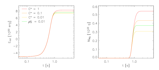
Figure 1: Single-octant simulations with $N=128^{3}$, $C_{\mathrm{e}}=10^{4}$ and various choices of $C^{\ast}$. Plotted are the evolution of the total energy and the integrated mass of intermediate mass elements, respectively. Also shown is a reference simulation, in which the burning process was stopped at the density threshold $\rho_{9}\leq 0.01$.

Table 2: Total energy release and masses of burning products at $t=5.0\,\mathrm{s}$ for the simulations shown in Fig. 1

.

	$E_{\mathrm{nuc}}\,[10^{51}\,\mathrm{erg}]$	$E_{\mathrm{kin}}\,[10^{51}\,\mathrm{erg}]$	$M_{\mathrm{Ni}}/M_{\sun}$	$M_{\mathrm{Mg}}/M_{\sun}$
$\rho_{9}^{\ast}=0.01$	1.261	0.753	0.707	0.188
$C^{\ast}=0.01$	1.235	0.727	0.708	0.155
$C^{\ast}=0.1$	1.287	0.779	0.708	0.217
$C^{\ast}=1.0$	1.332	0.824	0.708	0.270

4 Numerical simulations

We investigated the effect of including burning with the extended level set prescription in a follow-up study of Schmidt & Niemeyer (2006). To that end, we modified the criterion for the termination of the burning process in the code as follows. From the values of $s_{\mathrm{lam}}$ and $\delta$ calculated by Timmes & Woosley (1992), we obtained $\tau_{\mathrm{nuc}}=\delta/s_{\mathrm{lam}}$ and linearly fitted $\log\tau_{\mathrm{nuc}}$ as a function of $\log\rho_{9}$ , where $\rho_{9}$ is the mass density in units of $10^{9}\,\mathrm{g/cm^{3}}$, for $\rho_{9}<1.0$. The power law resulting from this fit is

$$\tau_{\mathrm{nuc}}(\rho_{9})=\frac{4.146\cdot 10^{-11}\,\mathrm{s}}{\rho_{9}^{3.7417}}.$$ (17)

The data points as well as the corresponding values of the fit function are listed in Table 1. Evaluating $\tau_{\mathrm{nuc}}(\rho_{9})$ locally in each cell, it can be checked whether the criterion 16 is fulfilled for a certain prescribed constant $C^{\mathrm{\ast}}$. If the nuclear time scale becomes larger than the threshold given by the right-hand side, burning will be terminated. Since $\Delta\sim 10^{6}\,\mathrm{cm}$ and $q_{\mathrm{sgs}}\sim 10^{7}\,\mathrm{cm\,s^{-1}}$ after about one second, $C^{\ast}\Delta/q_{\mathrm{sgs}}\lesssim 0.1\,\mathrm{s}$. Thus, the power law 17 has to be somewhat extrapolated towards $\rho_{9}\approx 0.003$, which appears to be reasonable.

To begin with, we computed a series of single-octant simulations on grids consisting of $N=128^{3}$ cells with the code described in Schmidt et al. (2006b). Due to the hybrid geometry of these grids, with a fine-resolved uniform inner part and exponentially growing cell size in the outer part, in combination with the co-expanding grid technique introduced by (Röpke 2005), it was possible to study trends even with a relatively small number of grid cells. If we had chosen a higher resolution, the applicability of the level set method would have been constrained even further. This can be seen from the criterion (16) with the scaling law $q_{\mathrm{sgs}}\sim\Delta^{1/3}$. Since the nuclear time scale $\tau_{\mathrm{nuc}}$ gradually increases as the explosion progresses, lowering the cutoff length $\Delta$ implies that the termination point will be met earlier. On the other hand, a certain resolution is mandatory for capturing the large-scale production of turbulence by Rayleigh-Taylor instabilities. From the resolution study in Schmidt et al. (2006b) and the influence of doubling the resolution of thermonuclear supernova simulations with stochastic ignition discussed by Schmidt & Niemeyer (2006), we conclude that $128^{3}$ cells per octant are sufficient for arriving at a sensible estimate of the total amount of burning products.

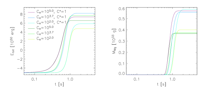
Figure 2: Evolution of the total energy and the integrated mass of intermediate mass elements, respectively, for several full-star simulations with $N=256^{3}$. For each value of the exponentiation parameter $C_{\mathrm{e}}$, which controls the number of ignitions events, either $\rho_{9}\leq 0.01$ or $\tau_{\mathrm{nuc}}\geq\Delta/q_{\mathrm{sgs}}$ (corresponding to $C^{\ast}=1.0$) was set for the termination of the burning process.

Table 3: Total energy release and masses of burning products at $t=5.0\,\mathrm{s}$ for the simulations shown in Fig. 2

.

	$C_{\mathrm{e}}$	$E_{\mathrm{nuc}}\,[10^{51}\,\mathrm{erg}]$	$E_{\mathrm{kin}}\,[10^{51}\,\mathrm{erg}]$	$M_{\mathrm{Ni}}/M_{\sun}$	$M_{\mathrm{Mg}}/M_{\sun}$
$\rho_{9}^{\ast}=0.01$	$10^{2}$	0.985	0.478	0.523	0.201
$\rho_{9}^{\ast}=0.01$	$5\cdot 10^{3}$	1.274	0.766	0.715	0.188
$\rho_{9}^{\ast}=0.01$	$10^{5}$	1.165	0.657	0.647	0.184
$C^{\ast}=1.0$	$10^{2}$	1.095	0.587	0.545	0.293
$C^{\ast}=1.0$	$5\cdot 10^{3}$	1.328	0.821	0.701	0.280
$C^{\ast}=1.0$	$10^{5}$	1.246	0.738	0.645	0.286

Applying the stochastic ignition procedure formulated by Schmidt & Niemeyer (2006), we selected a reference model with $C_{\mathrm{e}}=10^{4}$, where the parameter $C_{\mathrm{e}}$ adjusts the time scale of Poisson processes generating the ignition events in thin adjacent spherical shells. Depending on the choice of $C_{\mathrm{e}}$, the outcome of the explosion, in particular, the release of nuclear energy and the total mass of iron group elements is varying greatly. For $C_{\mathrm{e}}=10^{4}$, the total number of ignition events per octant is roughly $100$ and the yield of nuclear energy becomes nearly maximal (see Table 1 and Fig. 1 in Schmidt & Niemeyer (2006)). We repeated this simulation with the same initial white dwarf model and parameter settings, except for the termination of the burning process as explained above, using three different values of $C^{\ast}$.

The time evolution of the total amount of intermediate mass elements (represented by ²⁴Mg) plotted in the right panel of Fig. 1 clearly shows the influence of the burning termination criterion. Assuming $C^{\ast}=1$, the total magnesium mass $M_{\mathrm{Mg}}$ at $t=5.0\,\mathrm{s}$ increases by $44\,\%$ compared to the reference simulation (see Table 2, in which burning ceases for $\rho_{9}\leq\rho_{9}^{\ast}=0.01$. One should note that this is only a lower bound, because $C^{\ast}=1$ indicates that the broken-reaction-zones regime has just been entered and volume burning at resolved scales, which cannot be treated with the present code, would consume even more carbon and oxygen. The mass of iron group elements (⁵⁴Ni), on the other hand, remains unaffected which, of course, reflects nickel being produced entirely within the flamelet regime at densities $\rho_{9}\geq 0.05$ while magnesium is stemming largely from distributed burning at lower densities. Even for $C^{\ast}=0.1$, meaning that the extended level set prescription breaks down well within the broken-reaction-zones regime, the yield of intermediate mass elements is still higher than in the case of the density threshold $\rho_{9}^{\ast}=0.01$. If $C^{\ast}=0.01$, on the other hand, $M_{\mathrm{Mg}}$ becomes slightly smaller. Since $C^{\ast}\ll 1$ implies a greatly reduced energy generation rate, the physical quenching of the flame brush would be nearly reached in this case and, as a consequence, only little volume burning could possibly follow. In this case, we can be fairly sure that the actual amount of burning products would be more or less what is seen in the simulation.

We also performed full-star simulations with $N=256^{3}$, for which $\Delta$ is initially the same as in the single-octant simulations. Varying the exponentiation parameter $C_{\mathrm{e}}$, the burning process was terminated once $\tau_{\mathrm{nuc}}\geq\Delta/q_{\mathrm{sgs}}$, i.e. $C^{\ast}=1.0$. The results in comparison to the corresponding simulations with the termination criterion $\rho_{9}\leq 0.01$ from (Schmidt & Niemeyer 2006) are plotted in Fig. 2. Because of the substantially larger mass of unburned carbon and oxygen that will be left over at the transition from iron group to intermediate mass element production if $C^{\ast}$ is smaller and, consequently, the ignition proceeds slower, one would expect $M_{\mathrm{Mg}}$ to increase with $C_{\mathrm{e}}$. However, the burning statistics listed in Table 3 clearly demonstrates that $M_{\mathrm{Mg}}$ is almost constant for varying $C_{\mathrm{e}}$. Hence, distributed burning appears to consume about the same amount of fuel independent of the state of the exploding star at the end of the flamelet regime.

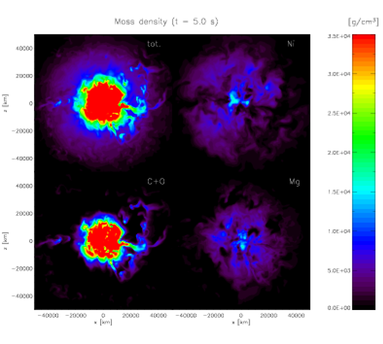
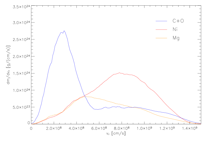
Figure 3: Total and fractional mass densities in a central section and the corresponding probability density functions in radial velocity space for a full-star simulation with $C_{\mathrm{e}}=10^{2}$ at $t=5.0\,\mathrm{s}$.

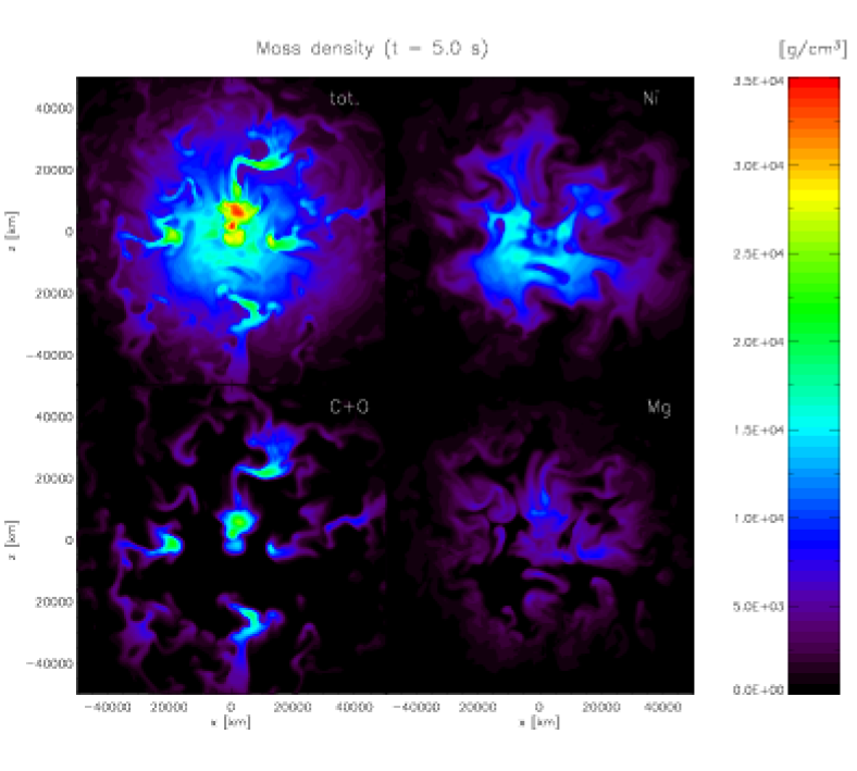
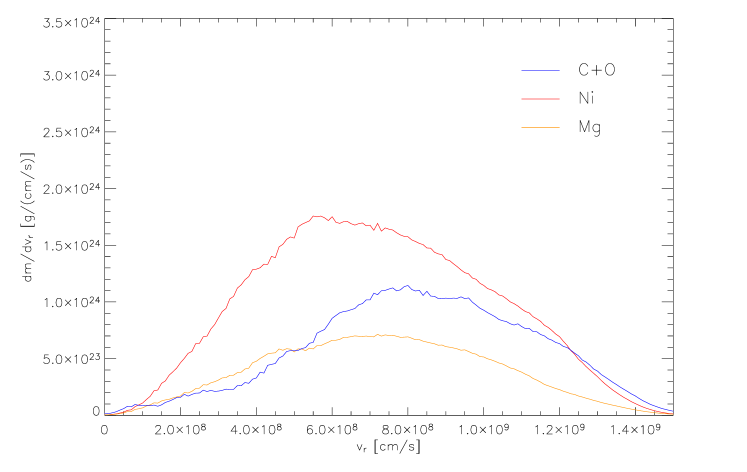
Figure 4: Total and fractional mass densities in a central section and the corresponding probability density functions in radial velocity space for a full-star simulation with $C_{\mathrm{e}}=5\cdot 10^{3}$ at $t=5.0\,\mathrm{s}$.

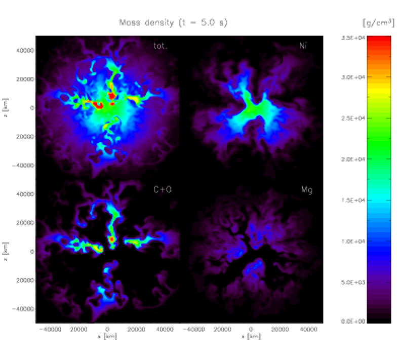
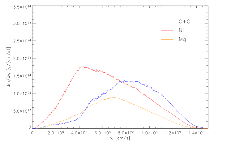
Figure 5: Total and fractional mass densities in a central section and the corresponding probability density functions in radial velocity space for a full-star simulation with $C_{\mathrm{e}}=10^{5}$ at $t=5.0\,\mathrm{s}$.

Fig. 3–5 show contour plots of the total mass density and the partial densities of C$+$O, Mg and Ni, respectively, in two-dimensional central sections at time $t=5.0\,\mathrm{s}$. In comparison to Fig. 2–4 in (Schmidt & Niemeyer 2006), which show the corresponding density contours in the simulations with the burning process terminated if $\rho_{9}\leq 0.01$, one can see that the explosion ejecta are substantially enriched in intermediate mass elements. This is also illustrated by the plots of the fractional masses as function of radial velocity in Fig. 3–5. Although the residuals of unburned material at low radial velocities, which have been plaguing the deflagration models, are still present in each case, it is likely the a significant further reduction would result from volume burning beyond the break-down of the level set description. Nevertheless, a non-negligible amount of carbon and oxygen at radial velocities larger than about $5000\,\mathrm{km/s}$ will be left over for any conceivable choice of parameters.

5 Conclusion

We have argued that the turbulent flame propagation speed in thermonuclear supernova simulations is given by the subgrid scale turbulent velocity even in the distributed burning regime. Moreover, the level set representation of the flame front remains valid beyond the flamelet regime provided that the width of the flame brush is smaller than grid resolution. In terms of time scales, this constraint corresponds the termination criterion (16).

Very little is known about the interaction between turbulence and the burning process in the broken-reaction-zones regime, in which turbulence is mixing fuel and ash faster than the nuclear reactions are progressing. Since the break-down of the level set description possibly occurs in this regime, we introduced the dimensionless parameter $C^{\ast}$ which specifies the reduction of the energy generation rate due to turbulent entrainment of fuel and ash. The limiting case $C^{\ast}\simeq 1$ corresponds to the thin-reaction-zones regime. In this regime, the flame is broadened due to the enhanced diffusivity in the preheating zone while the reaction zone is not significantly affected by turbulent eddies. As turbulence increasingly disturbs the reaction zone, $C^{\ast}$ diminishes. For $C^{\ast}\ll 1$, burning will be quenched.

Setting $C^{\ast}$ to values in the range from 0.01 to 1, we performed several supernova simulations with burning being terminated once (16) was fulfilled. In these simulations, we applied the stochastic ignition procedure described in (Schmidt & Niemeyer 2006). For $C^{\ast}\gtrsim 0.1$, a greater fraction of intermediate mass elements was produced as in reference simulations with termination of the burning process at the density threshold $\rho_{9}=0.01$. Remarkably, we found that $0.3M_{\sun}$ of intermediate mass elements was produced in the case $C^{\ast}=1.0$ independent of the rapidity of the ignition process. Consequently, the ignition process mainly determines the total mass of iron group elements, whereas the production of intermediate mass elements appears to depend solely on the progression of distributed burning.

Although a substantial increase of the amount of iron group elements might result from volume burning at resolved scales, which cannot be treated within the present methodology, it seems unlikely that the remaining fraction of carbon and oxygen would be consumed completely. For this reason, if clear indications of carbon residuals at least in certain type Ia supernovae were not found, delayed detonations would be an unavoidable conclusion. Even in this case, however, studying the physics of distributed burning in more detail might very well help to clarify the physical mechanism of the putative DDT. On the other hand, if burning was completed in the distributed mode in some SNe Ia, small-scale numerical models of burning in the broken-reaction-zones regime and explicit treatment of volume burning in large-scale supernova simulations would be the prerequisites for further progress.