Reconstruction of interacting dark energy models from parameterizations

Abstract

Models with interacting dark energy can alleviate the cosmic coincidence problem by allowing dark matter and dark energy to evolve in a similar fashion. At a fundamental level, these models are specified by choosing a functional form for the scalar potential and for the interaction term. However, in order to compare to observational data it is usually more convenient to use parameterizations of the dark energy equation of state and the evolution of the dark matter energy density. Once the relevant parameters are fitted it is important to obtain the shape of the fundamental functions. In this paper I show how to reconstruct the scalar potential and the scalar interaction with dark matter from general parameterizations. I give a few examples and show that it is possible for the effective equation of state for the scalar field to cross the phantom barrier when interactions are allowed. I analyze the uncertainties in the reconstructed potential arising from foreseen errors in the estimation of fit parameters and point out that a Yukawa-like linear interaction results from a simple parameterization of the coupling.

I Introduction

Recent data from type Ia supernovae (SNIa) Riess ; SNLS , cosmic microwave background (CMB) WMAP3y and large scale structure (LSS) SDSS all point to the fact that the universe has recently entered into a stage of accelerated expansion. This is an unexpected and revolutionary discovery that calls for new physics, since gravity is always an attractive force.

The simplest possibility to explain the acceleration of the universe is to postulate the existence of a cosmological constant of the right magnitude. While this assumption is still compatible with all available data, it is unsatisfactory on the grounds of the huge amount of fine tuning required. Hence, exploratory models with scalar fields possessing a varying non-zero vacuum energy density, usually called quintessence models reviews , have been studied as an alternative to the cosmological constant solution. One of the most important tasks ahead of observational cosmology is to devise methods and gather data to successfully and unequivocally distinguish between these two possibilities. Finding evidence for an evolving vacuum energy would be one of the greatest discoveries of the century.

What is the appropriate scalar potential that could reproduce the observed data? There has been a large number of papers dealing with the possibility of reconstructing the potential directly from the data NakamuraChiba ; HutererTurner ; Starobinsky ; SainiEtAl ; MBS ; Shinji ; HutererPeiris ; SLP ; LiHolzCooray and it is fair to say that any statement about the form of the potential depends upon some level of parameterization. The procedure has also been extended to reconstruct the potential and the form of the scalar-gravity coupling in the Jordan frame of a scalar-tensor gravity theory from data on luminosity distance and linear density perturbation BoisseauEtAl . More recently Guo, Ohta and Zhang GOZ studied the reconstruction of the scalar potential directly from parameterizations of the equation of state.

An intriguing possibility is that the scalar field is not totally decoupled from our world CarrolAmendola . Although the coupling to baryonic matter is severely constrained, it is still possible to allow for a coupling to non-baryonic dark matter. From a lagrangian point of view, these couplings could be of the form $W(\phi)m_{0}\bar{\psi}\psi$ or $W(\phi)m_{0}^{2}\varphi^{2}$ for a fermionic or bosonic dark matter represented by $\psi$ and $\varphi$ respectively, where the function $W$ of the quintessence field $\phi$ can in principle be arbitrary. In this scenario, the mass of the dark matter particles evolves according to some function of the dark energy field $\phi$, leading to an effective equation-of-state for the dark matter.

I will consider exploratory models for dark energy with a canonical scalar field coupled to dark matter. The lagrangian for this class of models is specified by the choice of two functions of the scalar field: the scalar field potential $V(\phi)$ and $W(\phi)$, the function that characterizes the coupling to dark matter. Specific forms for the scalar potential and for the interaction, such as power-law or exponential functions, have been extensively studied in the literature vamps ; DasCorasanitiKhoury ; HueyWendt .

However, instead of postulating a concrete model by choosing definite parametric forms for $V(\phi)$ and $W(\phi)$, it is often more convenient and completely equivalent to introduce a time-dependent parameterization for the dark energy equation of state $w_{DE}(a)$ and for a coupling function $\delta(a)$, where $a(t)$ is the scale factor of the universe. In fact, this approach is widely used in the uncoupled case in order to test for the time-variation of dark energy since it is much easier to compare to SNIa observations parametrizations . For the coupled case, an analysis of the impact of interactions on SNIa observations was performed using a specific coupling either in the Einstein AGP or Jordan NP frame of a scalar-tensor theory. More recently, parameterizations of $w_{DE}(a)$ and $\delta(a)$ were directly used to study the effects of DE-DM interactions on fits from SNIa data us .

Given a parameterization for $w_{DE}(a)$ and $\delta(a)$ with parameters fitted by observations, it is important to investigate the shape of the potential and interaction functions that results in those parameterizations. They define the fundamental model behind the parameterizations. In this article I will show how to reconstruct the scalar potential and the interaction from the general parameterized forms of the dark energy equation of state $w_{DE}(a)$ and a coupling function $\delta(a)$ and provide a few concrete examples.

II Reconstruction

The reconstruction program proposed here generalizes the one first developed by Ellis and Madsen EllisMadsen . I consider a spatially flat universe composed of three perfect fluids, namely dark energy, non-baryonic dark matter and baryons. The dark matter and baryons are non-relativistic pressureless fluids and Einstein’s equations result in:

$$H^{2} = \frac{8\pi G}{3}(\rho_{\phi}+\rho_{DM}+\rho_{b})$$ (1)

$$\dot{H}+H^{2} = -\frac{4\pi G}{3}(\rho_{\phi}+\rho_{DM}+\rho_{b}+3p_{\phi})$$

where $H=\dot{a}/{a}$ and the dark energy is described by a scalar field $\phi$ with energy density and pressure given by:

$$\rho_{\phi}=\frac{1}{2}\dot{\phi}^{2}+V(\phi)\;,\;\;\;p_{\phi}=\frac{1}{2}\dot{\phi}^{2}-V(\phi)$$ (2)

with a equation of state $w_{\phi}$ defined by $w_{\phi}=p_{\phi}/\rho_{\phi}$.

Conservation of the stress-energy tensor requires that the total energy density and pressure obey:

$$\dot{\rho}_{T}+3H(\rho_{T}+p_{T})=0.$$ (3)

Introducing the coupling function $\delta(a)$ between dark energy and dark matter as

$$\delta(a)=\frac{d\ln m_{\psi}(a)}{d\ln a}$$ (4)

results in the following equation for the evolution of the DM energy density $\rho_{DM}$ amendola :

$$\dot{\rho}_{DM}+3H\rho_{DM}-\delta(a)H\rho_{DM}=0.$$ (5)

Also, conservation of baryon number requires:

$$\dot{\rho}_{b}+3H\rho_{b}=0$$ (6)

and eq. (3) then implies that the dark energy density should obey

$$\dot{\rho}_{\phi}+3H(\rho_{\phi}+p_{\phi})+\delta(a)H\rho_{DM}=0.$$ (7)

Notice that the parameterization eq. (4) implies

$$W(\phi(a))=e^{-\int_{a}^{1}\delta(a^{\prime})d\ln a^{\prime}}$$ (8)

normalized such that $W(\phi(a=1))=1$.

Combining eqs. (2,7,8) one obtains a modified Klein-Gordon equation for the scalar field:

$$\ddot{\phi}+3H\dot{\phi}+\left(\frac{dV}{d\phi}+\frac{\rho_{DM}^{(0)}}{a^{3}}\frac{dW}{d\phi}\right)=0,$$ (9)

in agreement with Das, Corasaniti and Khoury DasCorasanitiKhoury .

One can now proceed to reconstruct the potential and the interaction for a given parameterization of the equation of state $w(a)$ and the interaction $\delta(a)$. The first step is to find the time variation of dark matter energy density, which is easily obtained by solving eq. (5):

$$\rho_{DM}(a)=\rho_{DM}^{(0)}a^{-3}e^{-\int_{a}^{1}\delta(a^{\prime})d\ln a^{\prime}},$$ (10)

where $\rho_{DM}^{(0)}$ is the non-baryonic DM energy density today. It is more useful to work with the variable $u=\ln a$, and one can write

$$\rho_{DM}(u)=\rho_{DM}^{(0)}e^{-3u}e^{-\int_{u}^{0}\delta(u^{\prime})du^{\prime}}.$$ (11)

The second step is to substitute $\rho_{DM}(u)$ into eq. (7), which in terms of $u$ reads:

$$\rho_{\phi}^{\prime}(u)+3(1+w_{\phi}(u))\rho_{\phi}(u)+\delta(u)\rho_{DM}(u)=0,$$ (12)

where ${}^{\prime}=d/du$, and find a solution $\rho_{\phi}(u)$ with initial condition $\rho_{\phi}(u=0)=\rho_{\phi}^{(0)}$, with $\rho_{\phi}^{(0)}$ being the dark energy density today.

In the third step one constructs the Hubble parameter:

$$\frac{H^{2}(u)}{H_{0}^{2}}=\Omega_{b}e^{-3u}+\Omega_{DM}e^{-3u}e^{-\int_{u}^{0}\delta(u^{\prime})du^{\prime}}+\Omega_{\phi}f(u),$$ (13)

where $\Omega_{X}=\rho_{X}^{(0)}/\rho_{c}^{(0)}$, the critical density today is $\rho_{c}^{(0)}=3H_{0}^{2}/(8\pi G)$ and $H_{0}$ is the Hubble constant. The function $f(u)$ that determines the evolution of the dark energy density is in general obtained numerically.

Having obtained the Hubble parameter, the fourth step consists in solving the evolution equation for the scalar field obtained from eqs. (1,2):

$$\left(\frac{d\tilde{\phi}}{du}\right)^{2}=-\frac{1}{4\pi}\left(\frac{d\ln H(u)}{du}+\frac{3}{2}(\Omega_{DM}(u)+\Omega_{b}(u))\right),$$ (14)

where $\tilde{\phi}=\phi/M_{Pl}$ is the scalar field in units of the Planck mass ($M_{Pl}=1/\sqrt{G}$) and

$$\Omega_{DM,b}(u)=\frac{\rho_{DM,b}(u)}{\rho_{\phi}(u)+\rho_{DM}(u)+\rho_{b}(u)}.$$ (15)

In the fifth step one numerically inverts the solution $\tilde{\phi}(u)$ in order to determine $u(\tilde{\phi})$ to finally obtain

$$\tilde{V}(\tilde{\phi})\equiv\frac{V(u(\tilde{\phi}))}{\rho_{c}^{(0)}} = \left(\frac{1}{3}\frac{H(u)}{H_{0}}\frac{dH/H_{0}}{du}+\frac{H^{2}(u)}{H^{2}_{0}}-\right.$$

$$\left.\frac{1}{2}\Omega_{b}e^{-3u}-\frac{1}{2}\Omega_{DM}e^{-3u}e^{-\int_{u}^{0}\delta(u^{\prime})du^{\prime}}\right)$$

and

$$W(u(\tilde{\phi}))=e^{-\int_{u}^{0}\delta(u^{\prime})du^{\prime}}.$$ (17)

This completes the reconstruction procedure. I will now work out some examples of this procedure. I adopt $\Omega_{\phi}=0.7$, $\Omega_{DM}=0.25$ and $\Omega_{b}=0.05$ in the following. In all examples I integrate the field equation starting from $u_{i}=-1.8$, corresponding to $z_{i}=5.05$ and I arbitrarily set $\tilde{\phi}(u_{i})=-1$.

III Examples

III.1 Constant $w_{\phi}$ and $\delta$

I start by considering the simple example of a constant equation of state $w_{\phi}$ and constant coupling $\delta$. In order to gain some intuition, I first show in fig. 1 the reconstructed potential for $w_{0}=-0.99$ and $\delta=0$. As expected, the scalar field evolves slowly in a very flat potential. Notice that the potential energy is slightly below $0.7\rho_{c}$ today due to the small kinetic energy of the scalar field.

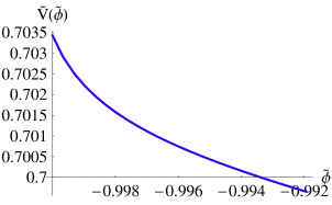
Figure 1: Reconstructed potential for $w_{\phi}=-0.99$ and $\delta=0$.

I now turn on the interaction. In this case one has AmendolaCamposRosenfeld :

$$\rho_{DM}(a)=\rho_{DM}^{(0)}a^{-3+\delta},$$ (18)

and the solution to eq.(7) is:

$$\rho_{\phi}(a)=\rho_{\phi}^{(0)}a^{-3(1+w_{\phi})}+\frac{\delta}{\delta+3w_{\phi}}\rho_{DM}^{(0)}\left(a^{-3(1+w_{\phi})}-a^{-3+\delta}\right).$$ (19)

The first term of the solution is the usual evolution of DE without the coupling to DM. From this solution it is easy to see that one must require a positive value of the coupling $\delta>0$ in order to have a consistent positive value of $\rho_{\phi}$ for earlier epochs of the universe. This feature remains in the case of varying $w_{\phi}$ and in the rest of the paper I will assume that $\delta$ is positive.

In fig. 2 I show the effects of the coupling in the reconstructed potential. I use $w_{0}=-0.9$ and $\delta=0,0.05$ and $0.1$. The scalar potential becomes steeper for larger values of the coupling due to the different dynamics introduced by the DE-DM coupling.

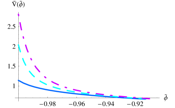
Figure 2: Reconstructed potential for $w_{\phi}=-0.9$ and $\delta=0$ (solid), $\delta=0.05$ (dashed) and $\delta=0.1$ (dot-dashed).

One might have expected that the introduction of the coupling could allow the possibility of having a phantom equation of state, $w_{\phi}<-1$. However, it is easy to show that one can write eq. (14) for both the uncoupled and coupled cases as:

$$\left(\frac{d\tilde{\phi}}{du}\right)^{2}=\frac{3}{8\pi}\left(1+w_{\phi}(u)\right)\Omega_{\phi}(u)$$ (20)

in the general case of a time-varying equation of state and hence, in order to have a real scalar field one must consider only $w_{\phi}(u)\geq-1$.

However, the fitter who is unaware of the interaction would instead find an effective equation of state $w_{eff}(u)$ defined implicitly by:

$$\rho_{\phi}^{(0)}e^{-3(1+w_{eff}(u))u}+\rho_{DM}^{(0)}e^{-3u}=\rho_{\phi}(u)+\rho_{DM}^{(0)}e^{(-3+\delta)u}.$$ (21)

In fig. 3 I show that the effective equation of state can in fact cross the phantom barrier. This possibility was also recently pointed out in the context of scalar-tensor theories of gravity tricked .

Figure 3: Effective equation of state for $w=-0.9$ and $\delta=0.1$.

One can also easily reconstruct the interaction $W(\tilde{\phi})$ in this simple case:

$$W(\tilde{\phi}(u))=e^{\delta u},$$ (22)

which of course guarantees that $W(\tilde{\phi}(u=0))=1$ as required. In fig. 4 I plot the reconstructed interaction term for $w=-0.9$ and $\delta=0.05,\;0.1$ and also for $w=-0.99$ and $\delta=0.1$. Notice that the interaction increases with time, corresponding to a mass that decreases with increasing redshift. One can see that the interaction term becomes steeper with increasing $\delta$ and decreasing $w$.

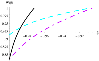
Figure 4: Reconstructed interaction for $w=-0.9$ and $\delta=0.05$ (dashed line), $\delta=0.1$ (dot-dashed line) and $w=-0.99$ and $\delta=0.1$ (solid line).

III.2 Variable $w_{\phi}$ and constant $\delta$

I now analyze the potential reconstructed from the commonly used 2-parameter description of the equation of state paramet :

$$w_{\phi}(a)=w_{0}+w_{1}(1-a).$$ (23)

A recent fit to SNIa, CMB and LSS data obtained (without DE perturbation) fit :

$$w_{0}=-1.098^{+0.078}_{-0.080},\;\;\;w_{1}=0.416^{+0.293}_{-0.153}$$ (24)

Hence I will assume that it is possible to fit the 2-parameter equation of state with a 1-$\sigma$ precision of $\delta w_{0}=0.08$ and $\delta w_{1}=0.20$. For illustration purposes, I will take the central values $w_{0}=-0.91$ and $w_{1}=0.4$ and study the effects of dark energy interaction in the reconstruction of the potential. In fig. 5 I show the allowed region in the potential form arising from the 1-$\sigma$ uncertainties in the estimation of the equation of state parameters. This region therefore gives an idea of the uncertainty one can expect in the reconstructed potential given the foreseen errors in the fit parameters.

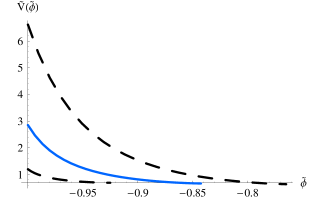
Figure 5: Reconstructed potential for $w_{0}=-0.91$, $w_{1}=0.4$ and $\delta=0$ (solid line). The allowed region from the $1-\sigma$ uncertainties in the estimation of the equation of state parameters is the region between the dashed lines.

In fig. 6 I show the effect of interaction with $\delta=0.1$ on the allowed region in the potential form arising from the $1-\sigma$ uncertainties in the estimation of the equation of state parameters.

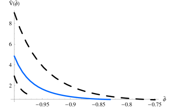
Figure 6: Reconstructed potential for $w_{0}=-0.91$, $w_{1}=0.4$ and $\delta=0.1$ (solid line). The allowed region from the $1-\sigma$ uncertainties in the estimation of the equation of state parameters is the region between the dashed lines.

III.3 Constant $w_{\phi}$ and variable $\delta$

Finally, I analyze the case of a constant equation of state and an interaction parameterized by the function Waga :

$$\delta(a)=\delta_{0}\frac{2a}{1+a^{2}},$$ (25)

which is well behaved in the past as well as in the future and $\delta(a=1)=\delta_{0}$. In this case one finds:

$$\rho_{DM}(a)=\rho_{DM}^{(0)}a^{-3}e^{2\delta_{0}(\arctan(a)-\pi/4)}$$ (26)

The reconstructed potential is shown in fig. 7 for $w_{\phi}=-0.9$ and $\delta_{0}=0.1,0.2$. The interaction function is given by

$$W(u(\tilde{\phi}))=e^{2\delta_{0}(\arctan(e^{u(\tilde{\phi})})-\pi/4)}$$ (27)

and it is plotted in fig. 8. Notice that in this example the interaction function has an approximate Yukawa-like linear form, even more so for the $\delta_{0}=0.2$ case.

Figure 7: Reconstructed potential for constant $w=-0.9$, and $\delta_{0}=0.1$ (solid line) and $\delta_{0}=0.2$ (dashed line).

Figure 8: Reconstructed interaction function for constant $w=-0.9$, and $\delta_{0}=0.1$ (solid line) and $\delta_{0}=0.2$ (dashed line).

IV Conclusions

It is natural to study models where the dark energy field is not totally separated from the rest of the world. In principle, it can interact with dark matter and this possibility has interesting consequences in the evolution of the universe, such as a mass-varying cold dark matter particle with a non-zero effective equation of state.

In order to compare these models to observations it is more convenient to use parameterizations of the dark energy equation of state and the coupling to dark matter. However, once the parameters are estimated it is important to find the fundamental lagrangian of the theory, that is, to determine the functional form of the scalar potential and its interaction with dark matter.

I showed in this paper how to reconstruct the scalar potential and the scalar interaction with dark matter from general parameterizations. For illustration purposes some examples are worked out. Uncertainties in the reconstruction due to uncertainties in the estimation of parameters are analyzed. It is pointed out that the phantom barrier can be crossed if the fit does not take into account interactions and that a Yukawa-like linear interaction results from a simple parameterization of the coupling.

More precise data from CMB, SNIa and LSS from different collaborations is expected to arrive in the near future. These data can be used to estimate the parameters of simple parameterizations and the procedure shown here can at least point towards the underlying fundamental model describing our universe.

References

- (1) A. G. Riess et al., Astrophys. J. 607, 665 (2004).
- (2) P. Astier et al., Astron. Astrophys. 447, 31 (2006).
- (3) D. N. Spergel et al., Astrophys. J. Supp. 148, 175 (2003), and astro-ph/0603449.
- (4) See, e.g., M. Tegmark et al., astro-ph/0608632.
- (5) For comprehensive reviews, see P. J. E. Peebles and B. Ratra, Rev. Mod. Phys. 75, 559 (2003); T. Padmanabhan, Phys. Rept. 380, 235 (2003).
- (6) A. A. Starobinsky, JETP Lett. 68, 757 (1999).
- (7) T. Nakamura and T. Chiba, Mon. Not. R. Astron. Soc. 306, 696 (1999); Phys. Rev. D62, 121301 (2000).
- (8) D. Huterer and M. S. Turner, Phys. Rev. D60, 081301 (1999).
- (9) T. D. Saini, S. Raychudury, V. Sahni and A. A. Starobinsky, Phys. Rev. Lett. 85, 1162 (2000).
- (10) I. Maor and R. Brustein, Phys. Rev. D67, 103508 (2003).
- (11) S. Tsujikawa, Phys. Rev. D72, 083512 (2005).
- (12) D. Huterer and H. V. Peiris, astro-ph/0610427.
- (13) M. Sahlén, A. R. Liddle and D. Parkinson, astro-ph/0610812.
- (14) C. Li, D. E. Holz and A. Cooray, astro-ph/0611093.
- (15) B. Boisseau, G. Esposito-Farese, D. Polarsky and A. A. Starobinsky, Phys. Rev. Lett. 85, 2236 (2000).
- (16) Z. K. Guo, N. Ohta and Y. Z. Zhang, Phys. Rev. D72, 023504 (2005);
- (17) S. M. Carroll, Phys. Rev. Lett. 81, 3067 (1998); L. Amendola, Phys. Rev. D62, 043511 (2000).
- (18) G. W. Anderson and S. M. Carrol, astro-ph/9711288 (unpublished); J. A. Casas, J. García-Bellido and M. Quirós, Class. Quantum Grav. 9, 1371 (1992); G. R. Farrar and P. J. E. Peebles, Astrophys. J. 604, 1 (2004); M. B. Hoffman, astro-ph/0307350 (unpublished); L. Amendola, Phys. Rev. D 62, 043511 (2000); L. Amendola and D. Tocchini-Valentini, Phys. Rev. D 64, 043509 (2001); L. Amendola, Mon. Not. Roy. Astron. Soc. 342, 221 (2003); M. Pietroni, Phys. Rev. D 67, 103523 (2003); D. Comelli, M. Pietroni and A. Riotto, Phys. Lett. B 571, 115 (2003); U. França and R. Rosenfeld, Phys. Rev. D 69, 063517 (2004).
- (19) S. Das, P. S. Corasaniti and J. Khoury, Phys. Rev. D73, 083509 (2006).
- (20) G. Huey and B. D. Wandelt, Phys. Rev. D74, 023519 (2006).
- (21) See, e.g. S. Nesseris and L. Perivolaropoulos, Phys. Rev. D70, 043531-1 (2004); L. Perivolaropoulos, Phys. Rev. D71, 063503 (2005).
- (22) L. Amendola, M. Gasperini and F. Piazza, JCAP 0409, 14 (2004).
- (23) L. Perivolaropoulos, JCAP 0510, 001 (2005); S. Nesseris and L. Perivolaropoulos, astro-ph/0611238.
- (24) E. Majerotto, D. Sapone and L. Amendola, astro-ph/0410543; L. Amendola, G. C. Campos and R. Rosenfeld, astro-ph/0610806.
- (25) G. F. R. Ellis and M. S. Madsen, Class. Quantum Grav. 8, 667 (1991); see also T. Padmanabhan and T. R. Choudhury, Mon. Not. Roy. Astron. Soc. 344, 823 (2003).
- (26) The formal correspondence to a scalar-tensor theory in the Einstein frame can be obtained by identifying , where is a function determined by the non-minimal coupling of the scalar field to the Ricci scalar in the Jordan frame. See, e.g., L. Amendola, Mon. Not. Roy. Astron. Soc. 312, 521 (2000).
- (27) S. M. Carrol, A. D. Felice and M. Trodden, Phys. Rev. D71, 023525 (2005).
- (28) M. Chevallier and D. Polarski, Int. J. Mod. Phys. D10, 213 (2001); E. V. Linder, Phys. Rev. Lett. 90, 091301 (2003).
- (29) J. Q. Xia, G. B. Zhao, B. Feng, H. Li and X. Zhang, Phys. Rev. D73, 063521 (2006).
- (30) L. Amendola, G. C. Campos and R. Rosenfeld, second reference in us .
- (31) I would like to thank Ioav Waga for suggesting this parameterization for the coupling .