Dark Energy is the Cosmological Quantum Vacuum Energy of Light Particles.
The Axion and the Lightest Neutrino

Abstract

We uncover the general mechanism and the nature of the today dark energy (DE). This is only based on well known quantum physics and cosmology. We show that the observed DE today originates from the cosmological quantum vacuum of light particles which provides a continuous energy distribution able to reproduce the data. Bosons give positive contributions to the DE while fermions yield negative contributions. As usual in field theory, ultraviolet divergences are subtracted from the physical quantities. The subtractions respect the symmetries of the theory and we normalize the physical quantities to be zero for the Minkowski vacuum. The resulting finite contributions to the energy density and the pressure from the quantum vacuum grow as $\log a(t)$ where $a(t)$ is the scale factor, while the particle contributions dilute as $1/a^{3}(t)$, as it must be for massive particles. We find the explicit today dark energy equation of state $P=w(z)\;{\cal H}$: It turns to be slightly $w(z)<-1$ with $w(z)$ asymptotically reaching the value $-1$ from below. A scalar particle can produce the observed dark energy through its quantum cosmological vacuum provided: (i) Its mass is of the order of $10^{-3}$ eV = 1 meV, (ii) It is very weakly coupled, and (iii) it is stable on the time scale of the age of the universe. The axion vacuum thus appears as a natural candidate. The neutrino vacuum (especially the lightest mass eigenstate) can give negative contributions to the dark energy. We find that $w(z=0)$ is slightly below $-1$ by an amount ranging from $(-1.5\times 10^{-3})$ to $(-8\times 10^{-3})$ and we predict the axion mass be in the range between 4 and 5 ${\rm meV}$ . We find that the universe will expand in the future faster than the de Sitter universe, as an exponential in the square of the cosmic time. Dark energy today arises from the quantum vacuum of light particles in FRW cosmological space-time in an analogous way to the Casimir vacuum effect of quantum fields in Minkowski space-time with non-trivial boundary conditions.

(+) passed away https://chalonge-devega.fr/HdeV.html

(a): https://chalonge-devega.fr/sanchez/

I Introduction and Results

Since the discovery of the dark energy in the present universe descu , schmidt , an intense observational activity has improved our knowledge about it scp , mas , DES , and more activity is expected to provide new data and understanding eg. Euclid , LSST . Many different approachs and models have been proposed to explain the dark energy quinta , mnudt , revde , albrecht , frieman . For reviews and approachs on the dark energy see for example Refs. revde , quinta , mnudt , albrecht ; frieman .

As is by now well known, let us mention that there exist current discordances between different cosmological probes, mainly the discrepancy in the value of the Hubble constant $H_{0}:5.0\;\sigma$ between early universe indirect $H_{0}$ determinations and late universe direct measurements of $H_{0}$, and other stresses and anomalies of lower statistical significance, which are interesting in their own but are not the subject of this paper, see for example Ref abdalla2022snowmass and references therein. As is well known too, there exist theoretical discordances too, as the fine adjustment of the cosmological constant $\Lambda$, see for example Refs. albrecht , frieman and references therein. Clarification to this problem have been provided recently NSPRD2021 , NSIJMPA2019 : The huge difference between the observed value of $\Lambda$ today and the particle physics evaluated value $\Lambda_{Q}$ is correct and must be physically like that, because the two values correspond to the same physical magnitude but to two different vacuum states and cosmic eras: The observed $\Lambda$ value today corresponds to the classical/semiclassical, large and dilute (mostly empty) universe today, consistent with the very low observed $\Lambda$ value, ($10^{-122}$ in Planck units), while the computed value $\Lambda_{Q}$ ($10^{+122}$ in Planck units) corresponds to the small, highly dense and energetic quantum gravity universe in its far (trans-Planckian) past, and this is consistent with its extremely high, trans-Planckian, value. The two values are classical-quantum duals of each other in the sense of the classical-quantum (wave-particle) duality including gravity, and independently agree with a path integral gravity derivation NSIJMPD2019 , NSIJMPA2019 , NSPRD2021 .

In this paper we study the cosmological Quantum Field Theory (QFT) vacuum as dark energy, within a fundamental analytic framework with explicit and analytic results: eg the derivation of the dark energy equation of state and the future evolution of the universe. Moreover, from these results we extract too the implications and determination of the particles contributing to dark energy and compute their masses.

We show that the dark energy present today in the universe originates from the cosmological quantum vacuum of light particles in the meV mass scale. This is a vacuum effect which unavoidably appears when quantum fields evolve in a cosmological space-time. That is, dark energy today is generated by a mechanism based on well known quantum physics and cosmology. Bosons yield positive contributions to the dark energy while fermions give negative contributions.

We find that the scale of the contributions to the dark energy is of the order of

$$\frac{M^{4}}{2\,(4\pi)^{2}}\;\log z_{\,\rm dec}\;,$$ (1)

where $M$ is the particle mass and $z_{\rm dec}$ is the redshift when it decoupled from the early universe plasma.

Generally speaking, the energy of a quantum field is the sum of the vacuum contribution plus particle contributions. It is known that the vacuum energy of a quantum field dissipates into particles when the field evolves coupled to other fields or to itself nosmink -nosb2 . Dissipation into fermions is reduced by Pauli blocking nosf ; bhp . Electrons, protons and photons are coupled to photons and therefore, their vacuum energy dissipates through photon production well before recombination, that is, when the temperature of the universe was $1$ MeV or more. Unstable particles cannot produce long-lasting vacuum effects. Only a very weakly coupled stable particle can produce a vacuum energy contribution lasting for times of the order of the age of the universe, that is, a vacuum energy contribution measurable today.

Since the dark energy is known to be positive, bosons must dominate the cosmological vacuum energy. The scale of the boson mass must be in the meV range because the observed dark energy density has the value slac

$$\rho_{\Lambda}\;=\;\Omega_{\Lambda}\;\rho_{c}\;=\;(2.39\;{\rm meV})^{4}\quad,\quad 1\;{\rm meV}\;=\;10^{-3}\;{\rm eV}\;\;.$$ (2)

Spontaneous symmetry breaking of continuous symmetries is a natural way to produce massless scalars (Goldstone bosons) in particle physics. Furthermore, a slight violation of the corresponding symmetry can give a small mass to such scalar particle. Axions, majorons and familons have been proposed on these grounds axi0 , invi , majo .

In addition, the lightest neutrino can give a negative contribution to the dark energy.

Neutrinos are by now very well motivated particles from the point of view of particle physics, cosmology and astrophysics, eg dod , kt , gorbunov . For Majorana type neutrinos, neutrinos and antineutrinos coincide while for Dirac neutrinos, neutrinos and antineutrinos are distinct. It is not yet clear whether neutrinos are of Majorana or Dirac type and in this paper we discuss the implications for dark energy of both of them. Interestingly enough light meV neutrinos and the meV axion do appear here as a consequence of our results for the dark energy computed from first principles. For constraints on other types of neutrinos and other relativistic species or”dark radiation” see for example archidiacono and references therein.

Neutrinos in the universe are known to be free for temperatures $T\lesssim 1$ Mev which correspond to redshifts $z\lesssim 6\times 10^{9}$ dod , kt , gorbunov That is, we can describe their evolution as free fermions in the cosmological FRW universe.

Axions with masses $M\sim 1$ meV are free for temperatures $T\lesssim 10^{6}$ GeV which correspond to redshifts $z\lesssim 10^{19}$ axi . They can be considered as free scalars in the cosmological FRW universe. Both, the axion and neutrino decoupling happens during the radiation dominated era. Before decoupling, the non-negligeable interaction of the corresponding particles made dissipation important and therefore the vacuum energy can only become significant after decoupling. Therefore, we can restrict ourselves to study the free quantum field evolution in the cosmological space-time after decoupling.

• We investigate the evolution of scalars and fermions as an initial value problem (Cauchy problem) for the corresponding quantum fields on a cosmological space-time.

• We find that the initial temperature has a negligible effect on the vacuum energy for late times.

• Both axions and neutrinos can lead to vacuum effects lasting cosmological time scales. Any of the two heavier neutrino mass eigenstates $\nu_{2}$ and $\nu_{3}$ would produce a large negative dark energy in the $(50\;{\rm meV})^{4}$ range. Hence:

  (i) either the heavier neutrinos $\nu_{2}$ and $\nu_{3}$ annihilate with their respective anti-neutrinos in a time scale of the age of the universe,

  (ii) or a stable scalar particle with mass in the $\gtrsim 50$ meV range must be present in order to reproduce the observed value of the dark energy Eq.(2).

  However, we find in this paper that the possibility (ii) is inconsistent with the observed dark energy equation of state.

An effective four fermions interaction with strength characterized by $M^{\prime\,-2}$ where $M^{\prime}$ is a mass scale can make the heavier neutrinos unstable. The mass scale $M^{\prime}$ should be $M^{\prime}\lesssim 1$ MeV or $M^{\prime}\lesssim 10$ MeV for the direct and inverse neutrino mass hierarchies.

As shown in Section VIII the lightest meV neutrino remains the only neutrino contribution to the dark energy. The heavier neutrinos dissipate at the time of the age of the universe.

As shown in Section VII, the meV axion lifetime to decay into photons is much longer than the age of the universe. Dissipation of the energy in the cosmological quantum axion vacuum takes longer than the age of the universe too.

These results are unified in Section IX with both light meV particles contributing to dark energy together: meV axions and meV light neutrinos, Table 1 summarizes their contributions, together with the computed equation of state.

On the other hand, let us mention that a global analysis of cosmological constraints on decaying axion-like particles (ALPs) performed recently Ref BalazsALPs2022 shows that ALPs are stable on cosmological time scales unless they would be heavy enough with masses $>300$ keV. This is an independent confirmation that $10^{-3}$ eV axions as shown in this paper are safely enough stable to be considered as the source of dark energy. Previously, ALPs have been proposed among other proposals, to be constituents of the cosmological energy density i.e. Ref FerreiraALPs2015 .

In conformal time $(\eta)$, the scalar and fermion fields rescaled by the scale factor $a(\eta)$ turn out to obey equations of motion similar to those in Minkowski space-time but with time-dependent masses

$$\chi^{\prime\prime}\;-\;\nabla^{2}\chi\;+\;\left[\;M^{2}\;a^{2}(\eta)\;-\;\frac{a^{\prime\prime}(\eta)}{a(\eta)}\;\right]\chi({\vec{x}},\eta)\;=\;0\;,$$ (3)

(4)

$$\left[\;i\;{\not\!{\partial}}\;-\;m\;a(\eta)\;\right]\,\psi({\vec{x}},\eta)\,=\,0\;.$$ (5)

Here, $\chi$ and $\psi$ are, respectively, rescaled scalar and fermion fields, $\nabla^{2}$ is the usual flat space Laplacian and $i{\not\!{\partial}}$ is the usual Dirac differential operator in Minkowski space-time in terms of flat space-time Dirac matrices.

There are two widely separate scales in the field evolution in cosmological space-times:

• The fast scale is the microscopic quantum evolution scale,
  typically $\sim 1/M\sim 1/m$, where $M$ and $m$ are the scalar and fermion masses respectively.

• The slow scale is the Hubble scale $1/H$ of the universe expansion.
  When $M\sim m\gg H,\;M^{2}\gg a^{\prime\prime}(\eta)/a^{3}(\eta)$, and hence the scale factor can be considered as constant.

• Therefore, the cosmological quantum field evolution for the fields $\chi$ and $\psi$ is just the Minkowski evolution with effective masses $(M^{2}\,a^{2})$ and $(m\,a)$, respectively, as seen from Eq.(3).

Energy density, pressure, and field density express in field theory as products of the field operators and their derivatives at equal space-time points. Such expressions are ultraviolet divergent and need to be subtracted. The subtractions respect the symmetries of the theory and we normalize them such that the physical quantities are zero for the vacuum in Minkowski space-time. The finite resulting quantities grow as $\log a(\eta)$. This is analogous to the high-energy growth of renormalized one-loop Feynman graphs.

That is, the energy density and the pressure get contributions from the quantum vacuum that grow as $\log a(\eta)$ while the particle contributions dilute as $1/a^{3}(\eta)$, as it must be for massive particles.

We obtain for the vacuum energy density and pressure of scalar and fermion fields with mass $M$ and $m$, respectively the following results:

$$<{\cal H}>(\eta)\buildrel a(\eta)\;\gg\;a_{\rm dcs},\;a_{\rm dcf}\over{=}\frac{M^{4}}{2\,(4\,\pi)^{2}}\left[\;\log a(\eta)+b_{S}-\frac{1}{4}\;\right]-\frac{m^{4}}{(4\,\pi)^{2}}\;\mathcal{N}\;\left[\;\log a(\eta)+b_{F}-\frac{1}{4}\;\right],$$ (6)

$$<P>(\eta)\buildrel a(\eta)\;\gg\;a_{\rm dcs},\;a_{\rm dcf}\over{=}-\frac{M^{4}}{2\,(4\,\pi)^{2}}\;\left[\;\log a(\eta)+b_{S}+\frac{1}{12}\;\right]+\frac{m^{4}}{(4\,\pi)^{2}}\;\mathcal{N}\;\left[\;\log a(\eta)+b_{F}+\frac{1}{12}\;\right]$$ (7)

where $b_{S}$ and $b_{F}$ take into account the initial values of the scale factor $a_{\rm dcs}$ and $a_{\rm dcf}$ (at the decoupling time) of the scalars and fermions, respectively. $\mathcal{N}=1$ for Majorana fermions and $\mathcal{N}=2$ for Dirac fermions.

Therefore, we obtain for the equation of state the explicit expression:

$$w(\eta)\;\equiv\;\frac{<P>(\eta)}{<{\cal H}>(\eta)}\buildrel a(\eta)\;\gg\;a_{\rm dcs},\;a_{\rm dcf}\over{=}-1\,-\,\frac{1}{3}\,\left[\;\log a(\eta)\,-\,\frac{1}{4}\,+\,\frac{b_{S}-(\,2\;\mathcal{N}\;m^{4}/{M^{4}}\,)\;b_{F}}{1-(\,2\;\mathcal{N}\;m^{4}/{M^{4}}\,)}\;\right]^{-1}\;$$ (8)

That is, we find $w(\eta)<-1$ with $w(\eta)$ asymptotically reaching the value $-1$ from below.

It is convenient to express the scale factor in terms of the redshift. Taking into account that $b_{S}$ and $b_{F}$ contain the initial values of the scale factor yields,

$$a(\eta)\;e^{b_{S}}\;=\;\frac{1\;+\;z_{S}}{1+z}\quad,\qquad a(\eta)\;e^{b_{F}}\;=\;\frac{1\;+\;z_{F}}{1+z}\;,$$ (9)

where $z_{S}$ ($z_{F}$) is the redshift when the scalar (fermion) field decoupled. For neutrinos, $z_{F}\sim 6\times 10^{9}$, while for axions with mass $\sim 1$ meV, $z_{S}\sim 2.2\times 10^{18}$.

We find from Eqs.(6) and (9),

$$<{\cal H}>(z)=\frac{1}{2\,(4\,\pi)^{2}}\left\{M^{4}\;\log z_{S}-2\;\mathcal{N}\;m^{4}\;\log z_{F}-(M^{4}-2\;\mathcal{N}\;m^{4})\left[\;\log(1+z)+\frac{1}{4}\;\right]\right\}$$ (10)

(11)

$$<P>(z)=-\frac{1}{2\,(4\,\pi)^{2}}\left\{M^{4}\;\log z_{S}-2\;\mathcal{N}\;m^{4}\;\log z_{F}-(M^{4}-2\;\mathcal{N}\;m^{4})\left[\;\log(1+z)-\frac{1}{12}\;\right]\right\}$$

where we used that $z_{S}\gg 1,\;z_{F}\gg 1$.

We identify the vacuum energy density today $<{\cal H}>(z=0)$ with the observed dark energy $\rho_{\Lambda}$. We can then write Eqs.(6), (8) and (10) as:

$$\rho_{\Lambda}\;=\;\frac{1}{2\,(4\,\pi)^{2}}\left[\;M^{4}\left(\log z_{S}-\frac{1}{4}\right)-2\;\mathcal{N}\;m^{4}\left(\log z_{F}-\frac{1}{4}\right)\;\right]\;,$$ (12)

(13)

$$<{\cal H}>(\eta)\buildrel a(\eta)\;\gg\;a_{\rm dcs},\;a_{\rm dcf}\over{=}\rho_{\Lambda}\left[\;1\;+\;\beta_{\mathcal{N}}\;\log\frac{a(\eta)}{a_{0}}\;\right]\;,$$ (14)

(15)

$$w(\eta)\;+;\ 1\buildrel a(\eta)\;\gg\;a_{\rm dcs},\;a_{\rm dcf}\over{=}-\;\frac{\left(M^{4}\;-\;2\,\;\mathcal{N}\;m^{4}\right)}{6\,(4\,\pi)^{2}\;\rho_{\Lambda}\left[\;1\;+\;\beta_{\mathcal{N}}\;\log\frac{a(\eta)}{a_{0}}\;\right]}\;$$ (16)

where $a_{0}$ is the scale factor today and

$$\beta_{\mathcal{N}}\;=\;\frac{\displaystyle\left(1-\frac{2\;\mathcal{N}\;m^{4}}{M^{4}}\right)}{\displaystyle\log z_{S}\;-\;\frac{1}{4}\;-\;\left(2\;\frac{\;\mathcal{N}\;m^{4}}{M^{4}}\right)\left[\;\log z_{F}-\frac{1}{4}\;\right]\;}\;.$$ (17)

That is, the vacuum energy density at late times after decoupling grows as the logarithm of the scale factor and the equation of state asymptotically approaches $-1$ from below.

The equation of state as a function of z takes the form:

$$w(z)\;+\;1\;=\;-\;\frac{1}{3}\;\frac{\displaystyle\left(1-\frac{2\;\mathcal{N}\;m^{4}}{M^{4}}\right)}{\displaystyle\log z_{S}-\left(\frac{2\;\mathcal{N}\;m^{4}}{M^{4}}\right)\log z_{F}-\left(1-\frac{2\;\mathcal{N}\;m^{4}}{M^{4}}\right)\left[\;\log(1+z)+\frac{1}{4}\;\right]}$$ (18)

For $z=0$, it becomes today:

$$w(0)\;+\;1=-\;\frac{1}{3}\;\frac{\displaystyle\left(1-\frac{2\;\mathcal{N}\;m^{4}}{M^{4}}\right)}{\displaystyle\log z_{S}-\frac{1}{4}-\left(\frac{2\;\mathcal{N}\;m^{4}}{M^{4}}\right)\left[\;\log z_{F}-\frac{1}{4}\;\right]}=-\;\frac{1}{6\,(4\,\pi)^{2}\,\rho_{\Lambda}}\left(M^{4}-2\,\mathcal{N}\;m^{4}\right)\;$$ (19)

The scalar and fermion masses are constrained by the value of the dark energy today Eq.(2). This gives the positivity requirement:

$$M\;>\;\left(2\;\mathcal{N}\right)^{\frac{1}{4}}\;m\;,$$

as well as the expression for the mass of the scalar particle:

$$M\;=\;\displaystyle{\frac{10.1\;{\rm meV}}{\left(\;\log z_{S}\;-\;\frac{1}{4}\;\right)^{\,\frac{1}{4}}}\,\left[\;1\,+\,\mathcal{N}\;\left(\;\frac{m}{3.90\;{\rm meV}}\;\right)^{\!4}\;\right]^{\,\frac{1}{4}}}\;\;$$ (20)

The neutrino contribution to the dark energy can be ignored when $m\ll 1$ meV and when the vacuum neutrino contribution dissipates in the time scale of the age of the universe as mentioned before. The mass of the lightest neutrino is not yet known (only neutrino mass differences are known). We will consider that the lightest neutrino mass is either $m=3.2$ meV masanu , masanu2 or zero chica .

More specifically, we set $z_{S}\sim 2.2\times 10^{18}$ assuming the scalar field to be an axion with mass $\sim 1$ meV in Eqs.(19). (20).

• We therefore obtain for the axion mass $M$ and for the equation of state today the following values:

  $$3.96\;{\rm meV}\;<\;M\;<\;4.66\;{\rm meV}\;,$$ (21)

  (22)

  $$-\;0.00794\;<\;w(0)\;+\;1\;<\;-\;0.00156\;$$ (23)

  The left and right ends of the intervals in Eq.(21) correspond respectively to no neutrino contribution, and to the lightest neutrino contribution as a Dirac fermion with mass $m=3.2$ meV.

• We see that $w(0)$ is slightly below $-1$ by an amount ranging from $(-1.5\times 10^{-3})$ to $(-8\times 10^{-3})$, while the axion mass results between $4$ and $5$ meV which is within the range of axion masses allowed by astrophysical and cosmological constraints, eg. axiM .

  If the scalar particle is not the axion, the value of $z_{S}\gg 1$ will depend on the dynamics of such scalar particle.

• In general, we express the contribution of the quantum vacuum of light particles to the dark energy and pressure in terms of two parameters: the particle masses and the redshifts when they decoupled. There is also a dependence on the number of states per particle (1 for a scalar, $2\,\mathcal{N}$ for a fermion).

• We uncover in this paper the general mechanism producing the dark energy today. This mechanism is only based on well known quantum physics and cosmology. The observed dark energy in the universe today appears as a quantum vacuum effect only due to the (classical) cosmological space-time expansion. That is to say, dark energy in the present universe is a semiclassical gravity effect.

• The dark energy arises for a quantum field in the cosmological context in an analogous way the Casimir effect arises for a quantum field in Minkowski space-time with non-trivial boundary conditions in space.

• All physical (finite) results are independent of any energy cutoff as well as of the regularization method used.

• We obtain and solve in this paper the self- consistent Einstein-Friedmann equation for the scale factor when the dark energy dominates and the universe expansion accelerates. The growth of the energy density Eq.(6) as the logarithm of the scale factor implies an expansion faster than in de Sitter space-time. More precisely, we find that the Universe will reach in the future an asymptotic phase where it expands exponentially as

  $$a(t)\buildrel H_{0}\,t\;\gtrsim\;1\over{\simeq}a\,({\rm today})\;\exp{[\;c_{1}\,H_{0}\,t\,+\,c_{2}\;(H_{0}\;t)^{2}\;]}$$ (24)

  where

  $$c_{1}\;\equiv\;\sqrt{\Omega_{\Lambda}}\;=\;0.87\quad,\quad 0.00452\;<\;c_{2}\;<\;0.00872\;,$$ (25)

  and $H_{0}$ stands for the Hubble parameter today. The left and right ends of the interval for $c_{2}$ in Eq.(25) correspond respectively to the no neutrino contribution and to the lightest neutrino contribution as a Dirac fermion with mass $m=3.2$ meV.

• Notice that the time scale of the accelerated expansion is huge $\sim 1\,/\,H_{0}=13.4$ Gyr. In the exponent of Eq.(24) the quadratic term dominates over the linear term by a time $t\,\sim\,100\,/\,H_{0}$ to $200\,/\,H_{0}$.

  In this accelerated universe, we see from the Friedman equation and Eq.(6), that the Hubble radius $1/H$ decreases with time as $1\,/\,[\,H_{0}\;\sqrt{\log a(t)}\,]$.

This paper is organized as follows: In Sections II and III we review the dynamics of scalar and fermion fields on cosmological space-times, respectively. In Section IV we discus the quantum cosmological vacuum, the two point functions, et compute the main physical quantities from them. In Section V we find the vacuum energy density, pressure and the equation of state for late times and in Section VI we discuss their quantum nature. In Section VII we find dark energy as a result of the cosmological quantum vacuum contributions from meV light particles and their properties, masses and stability, axions are treated in this Section. In Section VIII we compute and analyze the neutrino contributions to dark energy: the lightest neutrino remains the only contribution. In Section IX we unify these results with both light meV particles together. We obtain the future self-consistent evolution of the universe in Section X. We discuss relevant related issues in Section XI, and we present our conclusions in Section XII. An Appendix is devoted to the equivalence between different regularization methods.

II Scalar Fields in Cosmological Space-Times

We consider a massive neutral scalar field $\varphi$ in a FRW geometry defined by the invariant distance

$$ds^{2}\;=\;dt^{2}\;-\;a^{2}(t)\;d\vec{x}^{2}\;.$$ (26)

The Lagrangian density is taken to be

$$\mathcal{L}\;=\;\frac{1}{2}\;\sqrt{-g}\;\Bigg{[}\;\dot{\varphi}^{2}\;-\;\left(\frac{\vec{\nabla}\varphi}{a}\right)^{2}-\;M^{2}\;\varphi^{2}\;\Bigg{]}\;.$$ (27)

It is convenient to use the conformal time $\eta$

$$\eta\;=\;\int\frac{dt}{a(t)}\;,$$

and the conformally rescaled field $\chi(\vec{x},\eta)$,

$$\chi(\vec{x},\eta)\;\equiv\;a(t)\;\varphi(\vec{x},t)\;.$$ (28)

The action (after discarding surface terms that do not affect the equations of motion) reads:

$$A\Big{(}\chi,\delta\Big{)}\;=\;\frac{1}{2}\;\int d^{3}x\;d\eta\;\Bigg{[}\;{\chi^{\prime}}^{2}-(\nabla\chi)^{2}-\mathcal{M}^{2}(\eta)\;\chi^{2}\;\Bigg{]}$$ (29)

where primes denote derivatives with respect to the conformal time $\eta$ and where

$$\mathcal{M}^{2}(\eta)\;=\;M^{2}\;a^{2}(\eta)\;-\;\frac{a^{\prime\prime}(\eta)}{a(\eta)}\;,$$ (30)

plays the role of an effective mass squared. Therefore, the rescaled field $\chi(\vec{x},\eta)$ obeys the equation of motion,

$$\chi^{\prime\prime}\;-\;\nabla^{2}\chi\;+\;\mathcal{M}^{2}(\eta)\;\chi\;=\;0\;.$$ (31)

The evolution of $\chi(\vec{x},\eta)$ is like that of a scalar field in Minkowski space-time with a time-dependent mass squared $\mathcal{M}^{2}(\eta)$.

The solution for the field $\varphi(\vec{x},t)$ can be Fourier expanded as follows,

$$\varphi(\vec{x},\eta)\;=\;\frac{1}{a(\eta)}\int\frac{d^{3}k}{(2\,\pi)^{3}\;2\;E_{0}}\;\left[\;a_{\vec{k}}\;\;\phi_{k}\;(\eta)\;e^{i\vec{k}\cdot\vec{x}}\;+\;a_{\vec{k}}^{\dagger}\;\;\phi_{k}^{*}\;(\eta)\;e^{-i\vec{k}\cdot\vec{x}}\;\right]$$ (32)

where

$$E_{0}\;\equiv\;\sqrt{\;k^{2}\;+\;\mathcal{M}^{2}_{i}\;}\;,$$

and $\mathcal{M}_{i}$ is the effective mass $\mathcal{M}(\eta)$ at the decoupling time (initial time) for the scalar field evolution. The mode functions $\phi_{k}(\eta)$ obey the evolution equations,

$$\left[\;\frac{d^{2}}{d\eta^{2}}\;+\;k^{2}\;+\;M^{2}\;a^{2}(\eta)\;-\;\frac{a^{\prime\prime}(\eta)}{a(\eta)}\;\right]\phi_{k}(\eta)\;=\;0\;.$$ (33)

We choose the initial state as the vacuum state which is here (at decoupling) a thermal equilibrium state at temperature $T$. However, as we see below [Eq.(101)], the effect of the initial temperature on the vacuum energy is negligible for late times. The Fock vacuum state $|0>$ is annihilated by the operators $a_{\vec{k}}$. Therefore, we have as initial conditions for the mode functions,

$$\phi_{k}(0)\;=\;1\quad,\quad\phi^{\prime}_{k}(0)\;=\;-\;i\;E_{0}\;.$$ (34)

These initial conditions describe the Bunch-Davies vacuum when they are applied at asymptotically earlier times in the past ($\eta\to-\infty$) BD , anom . See the discussion in Sec. XI here below.

The time-dependent creation and annihilation operators obey the canonical commutation rules,

$$\left[\;a_{\vec{k}}\;,\;a_{\vec{k}^{\prime}}^{\dagger}\;\right]\;=\;2\;E_{0}\;(2\,\pi)^{3}\;\delta(\vec{k}-\vec{k^{\prime}})\;.$$

The energy-momentum tensor for a scalar field is given by BD ,

$$T_{\mu\nu}\;=\;\partial_{\mu}\varphi\;\partial_{\nu}\varphi\;-\;\frac{1}{2}\;g_{\mu\nu}\left[\;\partial_{\lambda}\varphi\;\partial^{\lambda}\varphi\;-\;M^{2}\;\varphi^{2}\;\right]\;.$$ (35)

Its expectation value has the fluid form

$$<T_{S\;0}^{0}>\;\;=\;\;<{\cal H}_{S}>(\eta)\quad,\quad<T_{i}^{j}>\;\;=\;-\;\;\delta_{i}^{j}\,<P_{S}>(\eta)\;\;,$$

since we consider homogeneous and isotropic quantum states and density matrices. In conformal time the hamiltonian density and the pressure take the form

$${\cal H}_{S}(\eta)\;=\;\frac{1}{2\;a^{4}(\eta)}\left\{\;\left[\;\chi^{\prime}({\vec{x}},\eta)-a(\eta)\;H(\eta)\;\chi({\vec{x}},\eta)\,\right]^{2}+(\,\nabla\chi({\vec{x}},\eta)\,)^{2}+a^{2}(\eta)\;M^{2}\;\chi^{2}({\vec{x}},\eta)\;\right\}\;,$$ (36)

(37)

$${\cal H}_{S}\;+\;P_{S}(\eta)\;=\;\frac{1}{a^{4}(\eta)}\left\{\left[\;\chi^{\prime}({\vec{x}},\eta)-a(\eta)\;H(\eta)\;\chi({\vec{x}},\eta)\;\right]^{2}+\frac{1}{3}\;(\,{\nabla\chi}({\vec{x}},\eta)\,)^{2}\,\right\}\;,$$ (38)

where $H(\eta)$ stands for the Hubble parameter

$$H(\eta)\,\,\equiv\;\,\frac{d\;\ln a(t)}{dt}\;=\;\frac{1}{a^{2}(\eta)}\frac{da}{d\eta}\;.$$ (39)

It is convenient to consider the conformal energy and pressure,

$${\varepsilon}_{S}(\eta)\;\equiv\;a^{4}(\eta)\;<{\cal H}_{S}>(\eta)\quad,\quad p_{S}(\eta)\;\equiv\;a^{4}(\eta)\;<P_{S}>(\eta)\;.$$ (40)

We find the trace of the energy-momentum tensor from Eqs.(36),

$$a^{4}(\eta)\left[\,{\cal H}_{S}(\eta)-3\;P_{S}(\eta)\,\right]\;=\;a^{2}(\eta)\;M^{2}\;\chi^{2}-\left[\,(\chi^{\prime}-a\;h\;\chi)^{2}-(\nabla\chi)^{2}-a^{2}(\eta)\;M^{2}\;\chi^{2}\,\right]\;.$$ (41)

Ignoring the bracket term in the right hand side yields the virial theorem. Although this bracket term is nonzero, its space and time average is zero:

$$\frac{1}{\Delta}\int_{\eta}^{\eta+\Delta}d\eta\int d^{3}x\left[(\chi^{\prime}-a\;h\;\chi)^{2}-(\nabla\chi)^{2}-a^{2}(\eta)\;M^{2}\;\chi^{2}\right]\buildrel\Delta\gg 1/M\over{=}0\;.$$

In addition, this bracket can be neglected for late times as we shall see below.

Therefore, we have for the expectation values,

$${\varepsilon}_{S}(\eta)-3\,p_{S}(\eta)\;=\;M^{2}\;a^{2}(\eta)\;\Sigma_{S}(\eta)-a^{4}(\eta)\;V(\eta)$$ (42)

where

$$\Sigma_{S}(\eta)\;\equiv\;<\chi^{2}({\vec{x}},\eta)>\;=\;a^{2}(\eta)\;<\varphi^{2}({\vec{x}},\eta)>\;,$$ (43)

and $V$ stands for the expectation value of the virial

$$V(\eta)\;\equiv\;<(\chi^{\prime}-a\;h\;\chi)^{2}-({\nabla\chi})^{2}-a^{2}(\eta)\;M^{2}\;\chi^{2}>\;.$$

Using the equations of motion (31) we obtain for the time derivative of the energy density Eq.(40),

$$\frac{d\varepsilon_{S}}{d\eta}\;=\;\frac{1}{2}\;M^{2}\;\;\frac{da^{2}(\eta)}{d\eta}\,\;\Sigma_{S}(\eta)\;-\;a(\eta)\;H(\eta)\;V(\eta)\;.$$ (44)

This relation in conformal time implies the usual continuity equation in cosmic time

$$\frac{d}{dt}<{\cal H}_{S}>\;+\;\,3\;H(\eta)\;\left[\,<{\cal H}_{S}>\;+\;<P_{S}>\,\right]\;=\;0\;.$$ (45)

Therefore, from Eqs.(42) and (44) we see that there is only one independent quantity among $\varepsilon_{S}(\eta),\;p_{S}(\eta)$ and $\Sigma_{S}(\eta)$.

III Fermion Fields in Cosmological Space-Times

The Lagrangian density for fermions is taken to be anom

$$\mathcal{L}\;=\;\sqrt{-g}\;\;\overline{\Psi}\,\Big{[}\;i\,\gamma^{\mu}\;\mathcal{D}_{\mu}\Psi\;-\;m\;\Big{]}\,\Psi\;.$$ (46)

The $\gamma^{\mu}$ are the curved space-time Dirac $\gamma$ matrices and the fermionic covariant derivative is given by

$$\mathcal{D}_{\mu} = \partial_{\mu}\;+\;\frac{1}{8}\;[\;\gamma^{c}\;,\;\gamma^{d}_{;}]\;V^{\nu}_{c}\;\left(\;D_{\mu}V_{d\nu}\;\right)$$ (47)

$$D_{\mu}V_{d\nu} = \partial_{\mu}V_{d\nu}\;-\;\Gamma^{\lambda}_{\mu\nu}\;V_{d\lambda}$$

where the vierbein field is defined as

$$g^{\mu\,\nu}\;=\;V^{\mu}_{a}\;V^{\nu}_{b}\;\eta^{ab}\;,$$

$\eta_{ab}$ is the Minkowski space-time metric and the curved space-time matrices $\gamma^{\mu}$ are given in terms of the Minkowski space-time ones $\gamma^{a}$ by (Greek indices refer to curved space time coordinates and Latin indices to the local Minkowski space time coordinates)

$$\gamma^{\mu}\;=\;\gamma^{a}\;V^{\mu}_{a}\quad,\quad\{\gamma^{\mu},\gamma^{\nu}\}\;=\;2\;g^{\mu\nu}\;.$$

In conformal time the vierbeins $V^{\mu}_{a}$ are particularly simple

$$V^{\mu}_{a}\;=\;a(\eta)\;\delta^{\mu}_{a}\;,$$ (49)

where $a(\eta)\equiv a(t(\eta))$ is the scale factor as a function of the conformal time and we call $a(\eta=0)=a_{\rm dc}$. The Dirac Lagrangian density thus simplifies to the following expression

$$\sqrt{-g}\;\overline{\Psi}\left(\;i\;\gamma^{\mu}\;\mathcal{D}_{\mu}\Psi\;-\;m\;\right)\Psi\;=\;a^{\frac{3}{2}}\;\overline{\Psi}\;\left[\;i\;{\not\!{\partial}}\;-\;m\;a(\eta)\;\right]\left(a^{\frac{3}{2}}{\Psi}\right)$$ (50)

where $i{\not\!{\partial}}$ is the usual Dirac differential operator in Minkowski space-time in terms of flat space time $\gamma^{a}$ matrices.

Therefore, the Dirac equation in the FRW geometry is given by

$$\left[\;i\;{\not\!{\partial}}\;-\;m\;a(\eta)\;\right]\left[\;a^{\frac{3}{2}}\;{\Psi({\vec{x}},\eta)}\;\right]\;=\;0\;.$$ (51)

The solution $\Psi({\vec{x}},\eta)$ can be expanded in spinor mode functions as

$$\Psi(\vec{x},\eta)\;=\;\frac{1}{a^{\frac{3}{2}}(\eta)}\;\sum_{\lambda\,=\,\pm 1}\int\frac{d^{3}k}{(2\,\pi)^{3}\;2\;e_{0}}\;e^{i\vec{k}\cdot\vec{x}}\;\left[\;b_{\vec{k},\lambda}\,U_{\lambda}(\vec{k},\eta)\;+\;d^{\dagger}_{\,-\vec{k},\lambda}\,V_{\lambda}(-\,\vec{k},\eta)\;\right]\;,$$ (52)

where

$$e_{0}\;\equiv\;\sqrt{\;k^{2}\;+\;m^{2}\;a^{2}_{\rm dc}}\;,$$

and the spinor mode functions $U,V$ obey the Dirac equations

$$\left[\,i\;\gamma^{0}\;\partial_{\eta}\;-\;\vec{\gamma}\cdot\vec{k}\;-\;m\;a(\eta)\,\right]U_{\lambda}(\vec{k},\eta) = 0$$ (53)

$$\left[\,i\;\gamma^{0}\;\partial_{\eta}\;+\;\vec{\gamma}\cdot\vec{k}\;-\;m\;a(\eta)\,\right]V_{\lambda}(\vec{k},\eta) = 0\;.$$ (54)

The time-independent creation and annihilation operators obey the canonical anticommutation rules

$$\left\{b_{\vec{k},\,\lambda}\;,\;b^{\dagger}_{\vec{k^{\prime}},\,\lambda^{\prime}}\right\}\;\;=\,2\;e_{0}\;(2\,\pi)^{3}\;\delta(\vec{k}-\vec{k^{\prime}})\;\delta_{\lambda\;\lambda^{\prime}}\;,$$ (55)

(56)

$$\left\{d_{\vec{k},\,\lambda}\;,\;d^{\dagger}_{\vec{k^{\prime}},\lambda^{\prime}}\right\}\;=\;2\;e_{0}\;(2\,\pi)^{3}\;\delta(\vec{k}-\vec{k^{\prime}})\;\delta_{\lambda\;\lambda^{\prime}}\;.$$ (57)

Following the method of Refs. nosf , bhp , it proves convenient to write

$$U_{\lambda}(\vec{k},\eta) = {(e_{0}\;+\;m\;a_{\rm dc})}^{-\frac{1}{2}}\;\left[\,i\;\gamma^{0}\;\partial_{\eta}\;-\;\vec{\gamma}\cdot\vec{k}\;+\;m\;a(\eta)\,\right]f_{k}(\eta)\;\mathcal{U}_{\lambda}$$ (58)

$$V_{\lambda}(\vec{k},\eta) = {(e_{0}\;+\;m\;a_{\rm dc})}^{-\frac{1}{2}}\;\left[\,i\;\gamma^{0}\;\partial_{\eta}\;+\;\vec{\gamma}\cdot\vec{k}\;+\;m\;a(\eta)\,\right]g_{k}(\eta)\;\mathcal{V}_{\lambda}\;,$$ (60)

${(\;e_{0}+m\;a_{\rm dc}\;)}^{-\frac{1}{2}}$ being a normalization factor and $(\mathcal{U}_{\lambda},\;\mathcal{V}_{\lambda})$ being constant spinors nosf , bhp obeying

$$\gamma^{0}\;\mathcal{U}_{\lambda}\;=\;\mathcal{U}_{\lambda}\qquad,\qquad\gamma^{0}\;\mathcal{V}_{\lambda}\;=\;-\;\mathcal{V}_{\lambda}\qquad,\quad\lambda\;=\;\pm\;1\;.$$ (61)

More explicitly,

$$U_{\lambda}(\vec{k},\eta)\;=\;{(e_{0}\;+\;m\;a_{\rm dc})}^{-\frac{1}{2}}\;\left(\begin{array}[]{cc}\left[\,i\;f^{\prime}_{k}(\eta)\;+\;m\;a(\eta)\;f_{k}(\eta)\,\right]&0\\ 0&\lambda\;k\;f_{k}(\eta)\\ \end{array}\right)\mathcal{U}_{\lambda}\;\;,$$ (64)

(65)

(66)

$$V_{\lambda}(-\vec{k},\eta)={(e_{0}\;+\;m\;a_{\rm dc})}^{-\frac{1}{2}}\;\left(\begin{array}[]{cc}\lambda\;k\;g_{k}(\eta)&0\\ 0&\left[\,-i\;g^{\prime}_{k}(\eta)\;+\;m\;a(\eta)\;g_{k}(\eta)\,\right]\end{array}\right)\mathcal{V}_{\lambda}\;\;.$$ (69)

The mode functions $f_{k}(\eta),\;g_{k}(\eta)$ obey then the following equations of motion

$$\left[\;\frac{d^{2}}{d\eta^{2}}\;+\;k^{2}\;+\;m^{2}\;a^{2}(\eta)\;-i\;m\;a^{\prime}(\eta)\;\right]f_{k}(\eta) = 0$$ (70)

$$\left[\;\frac{d^{2}}{d\eta^{2}}\;+\;k^{2}\;+\;m^{2}\;a^{2}(\eta)\;+\;i\;m\;a^{\prime}(\eta)\;\right]g_{k}(\eta) = 0\;.$$ (72)

We choose the initial state for the fermion field as the vacuum state which is a thermal equilibrium state at temperature $T$ for the fermion. This Fock state $|0>$ is annihilated by the operators $b_{\vec{k},\lambda}$ and $d_{\vec{k},\lambda}$.

Therefore, we have as initial conditions for the mode functions nosf , bhp

$$f_{k}(0)\;=\;1\quad,\quad f^{\prime}_{k}(0)\;=\;-\;i\;e_{0}\quad,$$ (73)

(74)

$$g_{k}(0)\;=\;1\quad,\quad g^{\prime}_{k}(0)\;=\;+\;i\;e_{0}$$

These initial conditions describe the Bunch-Davies vacuum when they are applied at asymptotically earlier times in the past ($\eta\to-\infty$) BD , anom . See the discussion in Sec. XI below.

Eqs.(70)-(73) imply that

$$g_{k}(\eta)\;=\;f_{k}^{*}(\eta)\;.$$

That is, we have only one independent and complex mode function.

The scalar products of the spinors $U_{\lambda}(\vec{k},\eta),\;V_{\lambda}(\vec{k},\eta)$ take the values

$$U^{\dagger}_{\lambda}\;(\vec{k},\eta)\;U_{\lambda^{\prime}}(\vec{k},\eta)\;=\;2\;e_{0}\;\delta_{\lambda\;\lambda^{\prime}}$$ (75)

(76)

$$V^{\dagger}_{\lambda}\;(\vec{k},\eta)\;V_{\lambda^{\prime}}(\vec{k},\eta)\;=\;2\;e_{0}\;\delta_{\lambda\;\lambda^{\prime}}$$ (77)

As a consequence, the mode functions obey the relation nosf , bhp

$$|f^{\prime}_{k}(\eta)|^{2}-i\,m\;a(\eta)\;[f_{k}(\eta)\;{f^{\prime}}_{k}^{*}(\eta)-f^{\prime}_{k}(\eta)\;f_{k}^{*}(\eta)]+[k^{2}+m^{2}\;a^{2}(\eta)]\;|f_{k}(\eta)|^{2}=2\;e_{0}(e_{0}+m\;a_{\rm dc})\;,$$

which provides a conserved quantity.

The energy momentum tensor for a spin $1/2$ field is given by BD

$$T^{F}_{\mu\nu}\;=\;\frac{i}{2}\,\left[\,\overline{\Psi}\gamma_{(\mu}\stackrel{{\scriptstyle\leftrightarrow}}{{\mathcal{D}}}_{\nu)}\Psi\,\right],$$ (78)

and its expectation value has the fluid form

$$<{T_{F}}_{0}^{\,0}>\;\;=\;\;<{\cal H}_{F}>(\eta)\quad,\quad<{T_{F}}_{i}^{\,j}>\;\;=\;-\;\delta_{i}^{j}\;<P_{F}>(\eta)\;,$$

since we consider homogeneous and isotropic quantum states and density matrices.

More explicitly, the energy density in conformal time takes the form

$$<{\cal H}_{F}>(\eta)\;=\;\;<\Psi({\vec{x}},\eta)^{\dagger}\;H_{F}\;\Psi({\vec{x}},\eta)>\quad,$$ (79)

where the fermion hamiltonian $H_{F}$ is defined by

$$a(\eta)\;\gamma_{0}\;H_{F}\;=\;-\;i{\vec{\gamma}}\cdot{\vec{\nabla}}\;+\;m\;a(\eta)\;=\;{\vec{\gamma}}\cdot{\vec{p}}\;+\;m\;a(\eta)\;.$$ (80)

An analogous expression can be written for the pressure,

$$<P_{F}>(\eta)\;=\;\frac{1}{3\;a(\eta)}\;<{\bar{\Psi}}\;{\vec{\gamma}}\cdot{\vec{p}}\;\Psi>(\eta)\;.$$ (81)

Here too, it is convenient to consider the conformal energy and pressure,

$${\varepsilon}_{F}(\eta)\;\equiv\;a^{4}(\eta)\;<{\cal H}_{F}>(\eta)\quad,\quad p_{F}(\eta)\;\equiv\;a^{4}(\eta)\;<P_{F}>(\eta)\;.$$ (82)

We find the trace of the energy-momentum tensor from Eqs.(80), (81) and (82),

$$\varepsilon_{F}(\eta)\;-\;3\;p_{F}(\eta)\;=\;m\;a(\eta)\;\Sigma_{F}(\eta)\;,\qquad{\rm or}$$ (83)

(84)

$$<{\cal H}_{F}>(\eta)\;-\;3\;<P_{F}>(\eta)\;=\;m\;<{\bar{\Psi}}\Psi>(\eta)\;.$$

This is the expression of the virial theorem in the present context and

$$\Sigma_{F}(\eta)\;\equiv\;a^{3}(\eta)\;<{\bar{\Psi}}\Psi>(\eta)\;.$$ (85)

The above expressions for the energy density and pressure obey the usual continuity equation in cosmic time

$$\frac{d}{dt}<{\cal H}_{F}>\;+\;3\,H(\eta)\;\left(<{\cal H}_{F}>+<P_{F}>\right)=0\;,$$ (86)

In conformal time by using Eqs.(83)-(85) the continuity equation (86) becomes,

$$\frac{d\varepsilon_{F}}{d\eta}\;=\;m\;\frac{da(\eta)}{d\eta}\;\Sigma_{F}(\eta)\;.$$ (87)

We thus see from Eqs.(83) and (87) that there is only one independent quantity among $\varepsilon_{F}(\eta),\;{\mathcal{P}}_{F}(\eta)$ and $\Sigma_{F}(\eta)$.

IV The Cosmological Quantum Vacuum.

There are two widely separate scales in the field evolution in the cosmological space-time. The fast scale is the microscopic quantum evolution scale, typically $\sim 1/M\sim 1/m$. The slow scale is the Hubble scale $1/H$ of the universe expansion.

When $M\sim m\gg H$ we can consider that the scale factor is practically constant. Therefore, in conformal time the quantum field evolution is like the evolution in Minkowski space-time with a mass $M\;a(\eta)$ or $m\;a(\eta)$ for bosons or fermions, respectively [see Eqs.(30) and (51)].

The scalar and fermion densities follow as equal point limits of the scalar and fermion two point functions. That is, we consider the scale factor $a$ as a constant and obtain for the scalar two point function

$$G_{S}({\vec{x}}-{\vec{x}}^{\prime},\eta-\eta^{\prime},M\,a) \equiv <T\;\varphi({\vec{x}},\eta)\;\varphi({\vec{x}}^{\prime},\eta^{\prime})>\;=\frac{1}{a^{2}}\;\int\frac{d^{4}k}{(2\,\pi)^{4}}\;e^{-ik\cdot(x-y)}\frac{i}{k^{2}-a^{2}\;M^{2}+i\,0}=$$ (88)

$$= \frac{1}{(2\,\pi)^{2}}\;\frac{M}{z\;a}\;K_{1}(M\;a\;z)\quad,\quad z\equiv\sqrt{({\vec{x}}-{\vec{x}}^{\prime})^{2}-(\eta-\eta^{\prime})^{2}}\;,$$ (90)

where $K_{1}(x)$ is a modified Bessel function.

Eq.(88) is the zeroth order adiabatic approximation. It differs from the exact two point function by quantities of the order ${\cal O}(a^{\prime}(\eta)),\;{\cal O}(a^{\prime\prime}(\eta))$ etc.

We find from eq.(88) in the coincidence point limit :

$$G_{S}({\vec{x}}-{\vec{x}}^{\prime},\eta-\eta^{\prime},M\,a)\buildrel z\to 0\over{=}\frac{1}{(2\,\pi)^{2}}\,\left\{\,\frac{1}{z^{2}\;a^{2}}+\frac{1}{2}\,M^{2}\,\left[\,\log\left(M\;a\;z\right)+{\cal C}-\ln 2-\frac{1}{2}\,\right]\right\}[\,1+{\cal O}(M^{2}\,z^{2})\,].$$ (91)

where ${\cal C}=0.57721566\ldots$ is the Euler-Mascheroni constant. Eqs.(88)-(91) display the two point functions for the zero temperature vacuum. The effect of a non-zero temperature on the two point function is negligible for $a\gg 1$ as we show below [Eq.(101)].

The fermion two point function takes the form

$$<T\;\Psi({\vec{x}},\eta)_{\alpha}\;{\bar{\Psi}}({\vec{x}}^{\prime},\eta^{\prime})_{\beta}>\;\;=\;\;\frac{1}{a^{3}}\;\int\frac{d^{4}k}{(2\,\pi)^{4}}\;e^{-ik\cdot(x-y)}\;\;\frac{i\,({\not\!{k}}+a\;m)_{\alpha\;\beta}}{k^{2}-a^{2}\;m^{2}+i\,0}\;,$$ (92)

and hence,

$$G_{F}({\vec{x}}-{\vec{x}}^{\prime},\eta-\eta^{\prime},m\,a)\equiv\;<T\;{\bar{\Psi}}({\vec{x}},\eta)\;\Psi({\vec{x}}^{\prime},\eta^{\prime})>\;=-\;4\,m\;G_{S}({\vec{x}}-{\vec{x}}^{\prime},\,\eta-\eta^{\prime},\,m\,a),\qquad{\rm Dirac~{}Fermions}\;.$$ (93)

The minus sign in front arose from the anticommutation of the fermion fields going from Eq.(92) to Eq.(93). Here we used Eq.(88) and

$${\rm Tr}\;{\not\!{k}}\;=\;0\quad,\quad{\rm Tr}\;1\;=\;4\;.$$ (94)

That is, the factor $4=2\times 2$ in Eqs.(93) and (94) comes from the fermion and antifermion contributions times the number of helicities of a Dirac fermion. Hence, this factor $4$ becomes a factor $2$ for Majorana fermions:

$$G_{F}\,(\,{\vec{x}}-{\vec{x}}^{\prime}\,,\,\eta-\eta^{\prime}\,,\,m\,a\,)\;\equiv\;\;<{\bar{\Psi}}({\vec{x}},\eta)\;\Psi({\vec{x}}^{\prime},\eta^{\prime})>\;\;=\;-\,2\,m\;G_{S}\,({\vec{x}}-{\vec{x}}^{\prime}\,,\,\eta-\eta^{\prime},\,m\,a\,)\;.$$ (95)

We find in the coincidence point limit up to corrections $[\,1+{\cal O}(m^{2}\;z^{2})\,]$:

$$G_{F}({\vec{x}}-{\vec{x}}^{\prime},\eta-\eta^{\prime},m\,a)\buildrel z\to 0\over{=}-\,\frac{2\;\mathcal{N}\;m}{(2\,\pi)^{2}}\;\left\{\frac{1}{z^{2}\;a^{2}}\,+\,\frac{1}{2}\;m^{2}\,\left[\,\log\left(m\;a\;z\right)+{\cal C}-\ln 2-\frac{1}{2}\,\right]\right\}$$ (96)

Here, $\mathcal{N}=1$ for Majorana fermions and $\mathcal{N}=2$ for Dirac fermions.

In order to define the vacuum densities as the coincidence limits,

$$<\varphi^{2}>(\eta)\;\equiv\;\;<\varphi^{2}({\vec{x}},\eta)>\quad,\quad<{\bar{\Psi}}\Psi>(\eta)\;\equiv\;\;<{\bar{\Psi}}({\vec{x}},\eta)\;\Psi({\vec{x}},\eta)>$$

we have to subtract the singularities at $z=0$ in Eqs.(91) and (96). Subtracting the singularities leaves a finite $z$ independent piece. Requiring that the vacuum densities vanish in Minkowski space-time ($a=1$) we obtain,

$$<\varphi^{2}>(\eta)=\frac{M^{2}}{2\,(2\,\pi)^{2}}\;\left[\,\log a+b_{S}\;f_{S}(a)\,\right]\quad,\quad<{\bar{\Psi}}\Psi>(\eta)=-\frac{\mathcal{N}\;m^{3}}{(2\,\pi)^{2}}\;\left[\,\log a+b_{F}\;f_{F}(a)\,\right]\;$$ (97)

The functions $f_{S}(a)$ and $f_{F}(a)$ are finite and vanish for Minkowski space-time,

$$f_{S}(1)\;=\;0\quad,\quad f_{F}(1)\;=\;0\;.$$

We compute the terms $b_{S}\;f_{S}(a)$ and $b_{F}\;f_{F}(a)$ with the result:

$$f_{S}(\infty)\buildrel a(\eta)\;\gg\;a_{\rm dcs},\;a_{\rm dcf}\over{=}\;1\;+\;{\cal O}\left(\frac{1}{a^{2}}\right),\quad\quad f_{F}(\infty)\buildrel a(\eta)\;\gg\;a_{\rm dcs},\;a_{\rm dcf}\over{=}\;1\;+\;{\cal O}\left(\frac{1}{a^{2}}\right)\;.$$

When one performs an infinite subtraction at $z=0$, an additional finite subtraction can always be done. We recognize that the additional terms containing $b_{S}$ and $b_{F}$ can be absorbed in a finite multiplicative renormalization of the scale factor. That is, introducing $b_{S}$ and $b_{F}$ amounts to a scale transformation. We compute the coefficients $b_{S}$ and $b_{F}$ in terms of the subtraction scale in momentum space $(x\;M)$ for scalars and $(x\;m)$ for fermions, with the result

$$b_{S}(x)\;=\;b_{F}(x)\;=\;-\,\frac{1}{2}\;-\;\log x\;-\;\log a_{\rm dc}\;.$$

where $a_{\rm dc}$ stands for the scale factor at decoupling time (initial time). In summary, we have for the late time regime,

$$<\varphi^{2}>(\eta)\buildrel a(\eta)\;\gg\;a_{\rm dcs},\;a_{\rm dcf}\over{=}\frac{M^{2}}{2\,(2\,\pi)^{2}}\;\left[\,\log a(\eta)\,+\,b_{S}\,\right]\;=\;\frac{M^{2}}{2\,(2\,\pi)^{2}}\;\left[\,\log\frac{a(\eta)}{x\;a_{\rm dcs}}-\frac{1}{2}\,\right],$$ (100)

$$<{\bar{\Psi}}\Psi>(\eta)\buildrel a(\eta)\;\gg\;a_{\rm dcs},\;a_{\rm dcf}\over{=}-\frac{\mathcal{N}\;m^{3}}{(2\,\pi)^{2}}\;\left[\,\log a(\eta)\,+\,b_{F}\,\right]\;=\;-\frac{\mathcal{N}\;m^{3}}{(2\,\pi)^{2}}\;\left[\,\log\frac{a(\eta)}{x\;a_{\rm dcf}}-\frac{1}{2}\,\right]\;.$$

where $a_{\rm dcs}$ and $a_{\rm dcf}$ stand for the scale factor at the decoupling times (initial times) for the scalar and the fermion, respectively.

The two-point functions Eqs. (88) and (93) correspond to the zero temperature case. The singular pieces for $z\to 0$ are temperature independent. We can disregard the temperature dependent contributions to the two point functions since for large $a$ they decrease as

$$\sqrt{M}\;\left(\frac{T}{2\,\pi\;a}\right)^{\frac{3}{2}}\;e^{-\frac{M\;a}{T}}\,\to\,0\quad,\quad a\gg 1\;.$$ (101)

The scalar and fermion densities $<\varphi^{2}>(\eta)$ and $<{\bar{\Psi}}\Psi>(\eta)$ can be also computed as momentum integrals over the mode functions $\phi_{k}(\eta)$ and $f_{k}(\eta)$. In addition, the subdominant terms in $1/a^{2}(\eta)\;,\;{\dot{a}}(\eta)/a^{2}(\eta)\;,\ldots$ etc. can be obtained.

The equal points behaviour of the two point function Eqs.(91) and (96) is generic for any curved space-time when expressed as a function of the geodesic (squared) distance $\sigma\equiv z^{2}\;a^{2}$ between the two points. That is, the short distance behaviour is uniquely and universally determined by the local space-time geometry. It must be noticed that the divergences and finite pieces at $\sigma=0$ are of the same type as in Minkowski space-time. This is the so called Hadamard expansion for $\sigma\to 0$ and is equivalent to the adiabatic expansion. The coefficients of the divergent and finite parts are called Hadamard coefficients and they are known for generic space-times.

V Vacuum Energy Density and Pressure for Late Times

The total energy density $\varepsilon(\eta)$ and pressure ${\mathcal{P}}(\eta)$:

$$<{\cal H}>(\eta)\;=\;\;<{\cal H}_{S}>(\eta)\;\,+\;<{\cal H}_{F}>(\eta)$$ (102)

$$<P>(\eta)\;=\;\;<P_{S}>(\eta)\,\;+\;<P_{F}>(\eta),$$ (103)

can be computed in the late time regime using the virial theorem Eqs. (42) and (83), the continuity equation Eqs. (44) and (87) and the late time behaviour of the densities, Eq.(100).

We obtain after calculation for the energy density and pressure,

$$<{\cal H}>(\eta)\buildrel a(\eta)\;\gg\;a_{\rm dcs},\;a_{\rm dcf}\over{=}\frac{M^{4}}{2\,(4\,\pi)^{2}}\left[\log a(\eta)+b_{S}-\frac{1}{4}\;\right]-\frac{m^{4}}{(4\,\pi)^{2}}\;\mathcal{N}\,\left[\log a(\eta)+b_{F}-\frac{1}{4}\right]$$ (104)

$$<P>(\eta)\buildrel a(\eta)\;\gg\;a_{\rm dcs},\;a_{\rm dcf}\over{=}-\frac{M^{4}}{2\,(4\,\pi)^{2}}\;\left[\log a(\eta)+b_{S}+\frac{1}{12}\right]+\frac{m^{4}}{(4\,\pi)^{2}}\;\mathcal{N}\,\left[\log a(\eta)+b_{F}+\frac{1}{12}\right]$$ (105)

The decoupling (initial) times for the evolution of scalars and fermions can be different to each other. We have absorbed in $b_{S}$ and $b_{F}$ the corresponding initial values of the scale factor for scalars and fermions, respectively.

The positivity of the energy density impose the condition,

$$M^{4}\;>\;2\;\mathcal{N}\;m^{4}\;.$$

Notice that,

$$<P>(\eta)\;+\;<{\cal H}>(\eta)\buildrel a(\eta)\;\gg\;a_{\rm dcs},\;a_{\rm dcf}\over{=}-\;\frac{1}{6\,(4\,\pi)^{2}}\;\left[\,M^{4}\;-\;2\;\mathcal{N}\;m^{4}\,\right],$$

is time independent and independent of the finite subtraction coefficients $b_{S}$ and $b_{F}$ as well.

From Eq.(104) we obtain for the equation of state,

$$w(\eta)\;\equiv\;\frac{<P>(\eta)}{<{\cal H}>(\eta)}\buildrel a(\eta)\;\gg\;a_{\rm dcs},\;a_{\rm dcf}\over{=}-\;1\;-\;\frac{1}{3}\,\left[\;{\displaystyle\log a(\eta)\;-\;\frac{1}{4}\;+\;\frac{b_{S}-{(\;2\;\mathcal{N}\;m^{4}}/{M^{4}}\;)\;b_{F}}{1-{(\;2\;\mathcal{N}\;m^{4}}/{M^{4}}\;)}}\;\right]^{-1}$$ (106)

That is, we find $w(\eta)<-1$ with $w(\eta)$ asymptotically reaching the value $-1$ from below.

It is convenient to express the scale factor in terms of the redshift as

$$a(\eta)\;\exp{(b_{S})}\;=\;\frac{1\;+\;z_{S}}{1\;+\;z}\qquad,\qquad a(\eta)\;\exp{(b_{F})}\;=\;\frac{1\;+\;z_{F}}{1\;+\;z}\;,$$ (107)

where $z_{S}$ ($z_{F}$) is the redshift when the evolution of the scalar (fermion) become the one of a free field in the cosmological space-time. In terms of $z_{S}$ and $z_{F}$ Eqs.(104) read,

$$\begin{split}[\;2\,(4\,\pi)^{2}\;]\,<{\cal H}>(z)\;=\;M^{4}\,\log\;(1+z_{S})\;-\;2\,\mathcal{N}m^{4}\,\log\;(1+z_{F})\;-\\ -\;(M^{4}\,-\,2\,\mathcal{N}m^{4})\left[\;\log\,(1+z)\;+\;\frac{1}{4}\;\right]\,.\end{split}$$ (108)

$$\begin{split}[\;-\;2\;(4\;\pi)^{2}\;]\;<P>(z)\;=\;\;M^{4}\;\log\;(\;1+z_{S}\;)\;-\;2\;\mathcal{N}\;m^{4}\;\log\;(\;1\;+\;z_{F}\;)\;-\\ -\;(\;M^{4}\;-\;2\;\mathcal{N}\,m^{4}\;)\,\left[\,\log\;(\;1\;+\;z\;)\;-\;\frac{1}{12}\,\right]\,\end{split}$$ (109)

The equation of state (106) as a function of $z$ takes the form:

$$w(z)\,+\,1\;=\;-\frac{1}{3}\,\left(\;1-\frac{2\,\mathcal{N}\,m^{4}}{M^{4}}\;\right)\times\;\\ \times\;\left\{\,\log\;(1+z_{S})-\left(\frac{2\,\mathcal{N}\,m^{4}}{M^{4}}\right)\log\;(1+z_{F})-\left(1-\frac{2\,\mathcal{N}\,m^{4}}{M^{4}}\right)\left[\,\log\;(1+z)+\frac{1}{4}\,\right]\right\}^{-1}$$ (110)

The equation of state and the energy density become today:

$$w(z=0)+1\;=\;-\frac{1}{3}\,\left(1-\frac{2\;\mathcal{N}\;m^{4}}{M^{4}}\right)\left\{\,\log\,(1+z_{S})-\frac{1}{4}-\left(\frac{2\;\mathcal{N}\;m^{4}}{M^{4}}\right)\left[\,\log\,(1+z_{F})-\frac{1}{4}\,\right]\right\}^{-1}$$ (111)

$$<{\cal H}>(z=0)\;=\;\frac{1}{2\,(4\,\pi)^{2}}\left\{M^{4}\left[\,\log\,(1+z_{S})-\frac{1}{4}\,\right]-2\;\mathcal{N}\;m^{4}\left[\,\log\,(1+z_{F})-\frac{1}{4}\,\right]\right\}$$ (112)

The energy density at late times $\eta$ after decoupling and the energy density today are related by

$$<{\cal H}>(\eta)\buildrel a(\eta)\;\gg\;a_{\rm dcs},\;a_{\rm dcf}\over{=}<{\cal H}>(z=0)\;+\;\left(\frac{M^{4}-2\,\mathcal{N}\;m^{4}}{2\,(4\,\pi)^{2}}\right)\;\log\left(\frac{a(\eta)}{a_{0}}\right)$$ (113)

where we used Eqs.(104) and (111) and $a_{0}$ stands for the scale factor today.

We identify the vacuum energy density today $<{\cal H}>(z=0)$ with the observed dark energy $\rho_{\Lambda}$. We can then write,

$$<{\cal H}>(\eta)\;=\;\rho_{\Lambda}\left[\,1+\beta_{\mathcal{N}}\;\log\frac{a(\eta)}{a_{0}}\,\right]$$ (114)

where

$$\beta_{\mathcal{N}}\,\equiv\,\left(1-\frac{2\;\mathcal{N}\;m^{4}}{M^{4}}\right)\left\{\,\log\,(1+z_{S})\,-\,\frac{1}{4}\,-\,\left(\frac{2\;\mathcal{N}\;m^{4}}{M^{4}}\right)\left[\,\log\,(1+z_{F})\,-\,\frac{1}{4}\,\right]\,\right\}^{-1}$$ (115)

That is, the vacuum energy density at late times after decoupling grows as the logarithm of the scale factor. Moreover, the equation of state approaches $-1$ from below as:

$$w(\eta)+1\buildrel a(\eta)\;\gg\;a_{\rm dcs},\;a_{\rm dcf}\over{=}-\left(\frac{M^{4}-2\,\mathcal{N}\;m^{4}}{6\,(4\,\pi)^{2}\;\rho_{\Lambda}}\right)\left[\,1\,+\,\beta_{\mathcal{N}}\;\log\frac{a(\eta)}{a_{0}}\,\right]^{-1}.\;\;$$

The previous equations in this subsection generalize when there are several scalar and fermion fields just summing over their respective contributions. Let us consider the case of several scalars and fermions: This case is relevant to study whether the three neutrino mass eigenstates can contribute to the dark energy. Eqs.(111) become for $z_{S},\;z_{F}\gg 1$:

$$w(z\,=\,0)\;+\;1\;=\;-\;\frac{\sum_{j}M_{j}^{4}\;-\;2\;\mathcal{N}\;\sum_{i}m_{i}^{4}}{6\,(4\,\pi)^{2}\;\rho_{\Lambda}}\;,$$ (116)

(117)

$$\rho_{\Lambda}\;=\;\frac{1}{2\,(4\,\pi)^{2}}\left[\left(\log z_{S}-\frac{1}{4}\right)\sum_{j}M_{j}^{4}-2\;\mathcal{N}\left(\log z_{F}-\frac{1}{4}\right)\sum_{i}m_{i}^{4}\right]\;$$ (118)

where $j$ and $i$ label the species of scalars and fermions, respectively.

It is convenient to eliminate the sum of scalar masses $\sum_{j}M_{j}^{4}$ between eqs.(116) and (118) with the result,

$$w(z\,=\,0)\;+\;1\;=\;\frac{1}{(\log z_{S}-\frac{1}{4})}\left[\;-\frac{1}{3}\;+\;\frac{\mathcal{N}}{3\,(4\,\pi)^{2}}\;\frac{\sum_{i}m_{i}^{4}}{\rho_{\Lambda}}\;\log\frac{z_{S}}{z_{F}}\;\right]\;$$ (119)

We see in Eq.(119) that the scalar contributes to the equation of state today by the negative term $-1/[\,3\,(\,\log z_{S}-\frac{1}{4}\,)\,]$ while the fermions give for $z_{S}>z_{F}$ a positive contribution proportional to the sum of the fourth power of their masses.

VI The Quantum Nature of the Cosmological Vacuum.

Local observables as $<\varphi^{2}>,\;<{\bar{\Psi}}\Psi>$, the energy density and the pressure involve the product of field operators at equal points. This is identical to one-loop tadpole Feynman diagrams. Logarithmic dependence on the scale of the momenta is typical in one-loop renormalized Feynman diagrams IZ . Here, we analogously find a logarithm of the scale factor in Eqs.(100) and (104) through the same mechanisms at work in renormalized quantum field theory. Hence, the dark energy follows here as a truly quantum field vacuum effect. We stress quantum field effect and not just quantum effect because the infinite number of filled momentum modes in the vacuum as well as the subtraction of UV divergences play a crucial role in the vacuum late time behaviour. Here the quantum fields are not coupled neither self-coupled but they interact with the expanding space-time geometry.

Notice that these results Eqs.(100), (104) and (106) are valid for any expanding universe. They do not depend on the specific time dependence of the scale factor $a(\eta)$ provided it grows with $\eta$.

The quantum nature of the vacuum cosmological effects in the physical observables here are manifest from Eqs.(100) and (104),

$$<\varphi^{2}>(\eta) \sim\quad M^{2}\;\log a(\eta)\;=\;\frac{M^{2}\;c^{2}}{\hbar}\;\log a(\eta)\;=\;\frac{M\;c}{\lambda_{C}}\;\log a(\eta)\;,$$ (120)

$$<{\cal H}>(\eta) \sim\quad M^{4}\;\log a(\eta)\;=\;M\;c^{2}\left(\frac{M\;c}{\hbar}\right)^{3}\;\log a(\eta)\;=\;\frac{M\;c^{2}}{\lambda_{C}^{3}}\;\log a(\eta)\;$$ (122)

These quantities are of quantum nature since they depend on $\hbar$. There is no ‘classical contribution’ to the vacuum energy. Eq.(120) just means that the scale of the dark energy density is of one scalar rest mass per a volume equal to the cube of the Compton wavelength $\lambda_{C}$ for the scalar particle. Notice that $\lambda_{C}=[\hbar/{(M\;c)}]\simeq 0.05$ mm is almost a macroscopic length while the mass of the scalar particle $M\sim 4$ meV $=7.1\,10^{-36}$ g is extremely small (see below for the value of $M$).

VII Dark Energy from the Cosmological Quantum Vacuum.

Let us recall the current value for the dark energy density

$$\rho_{\Lambda}\;=\;\Omega_{\Lambda}\;\rho_{c}\;=\;3.28\times 10^{-11}\;({\rm eV})^{4}\;=\;(2.39\;{\rm meV})^{4}\;,$$ (123)

corresponding to

$$h\;=\;0.73,\qquad\Omega_{\Lambda}\;=\;0.76,\quad\;\text{and where}\;\;1\;{\rm meV}\;=\;10^{-3}\;{\rm eV}.$$ (124)

We take these values because they do correspond to direct, model independent and late universe observations, Refs descu , schmidt , scp , mas , DES , Riess2020 , Riess2021 , Riess2022 , and accordingly this paper deals directly with dark energy in the late universe; moreover, dark energy was discovered with such direct and model independent measurements in the late universe, Refs descu , schmidt , scp , mas . Other determinations of $h$ (eg. Ref Planck2020 Table 2, page 16) yield values $h=0.68$, $\Omega_{\Lambda}=0.69$. However, these are indirect, model dependent and early universe determinations of $h$ and $\Omega_{\Lambda}$. The difference between the determinations of $h$ in the late and in the early universe is an important problem by its own, eg. Ref. Riess2022 , although we do not treat this problem here.

Bosons give a positive contribution to the dark energy through the cosmological quantum vacuum while fermions give a negative contribution. Therefore, the boson contribution must dominate.

As discussed in Sec. VIII, the lightest neutrino certainly contributes to the cosmological quantum vacuum unless it dissipates. Definitely, a boson contribution is needed. The photon and graviton contributions are irrelevant since their masses are most probably zero and at most $m_{\;\gamma}\,<\,6\times 10^{-17}\;{\rm eV},\quad m_{\;\rm graviton}\,<\,4.7\times 10^{-23}\;{\rm eV}$  Abbott2019 .

Massless particles contribute to the energy-momentum tensor through the trace anomaly BD , anom . This contribution is of the order of $H_{0}^{4}$ where $H_{0}$ is the Hubble parameter today:

$$H_{0}\;=\;1.558\,\times\,10^{-33}\;{\rm eV}\;,$$ (125)

As a consequence, the massless particles contribution to the energy-momentum tensor is exceedingly small to explain the observed value of the dark energy.

• A scalar particle can produce the dark energy today Eq.(123) through its quantum cosmological vacuum provided:

• Its mass is of the order of $1$ meV and it is very weakly coupled.

• Its lifetime is of the order of the age of the universe.

Spontaneous symmetry breaking of continuous symmetries produces massless scalars as Goldstone bosons. If, in addition, this continuous symmetry is slightly violated the Goldstone boson acquires a small mass. This is the natural mechanism that generates light scalars and several particles have been proposed on these grounds in the past. The axion is certainly the one that caught more attention in the literature. Other proposed particles are the familons and the majorons majo , rneu .

The (invisible) axion invi (if it exists) is hence a candidate to be the source of dark energy.

Axions were proposed to solve the strong CP problem in QCD axi0 . Axions acquire a mass after the breaking of the Peccei-Quinn (PQ) symmetry when the temperature of the universe was at the PQ symmetry breaking scale $\sim f_{a}$ axi . All axion couplings are inversely proportional to $f_{a}$ and the axion mass is given by

$$M_{a}\;\simeq\;6\;\times\;\left(\frac{10^{9}\;{\rm GeV}}{f_{a}}\right){\rm meV}\;.$$ (126)

The following range (‘axion window’) is currently acceptable for the axion mass axiM , axiM2 :

$$10^{-3}\;{\rm meV}\;\lesssim\;M_{a}\;\lesssim\;10\;{\rm meV}\;$$ (127)

Therefore, this pseudoscalar particle has extremely weak coupling to gluons and quarks and hence it contributes to the cosmological quantum vacuum. For example, the axion-photon-photon coupling is given by

$$g_{a\;\gamma\;\gamma}\;\sim\;\frac{10^{-10}}{\rm GeV}\;\left(\frac{M_{a}}{1\;{\rm meV}}\right)\;$$ (128)

As a consequence, the axion lifetime to decay into photons is much longer than the age of the universe. Dissipation of the energy in the cosmological quantum axion vacuum takes longer than the age of the universe too.

• An axion with mass $\sim 1$ meV and hence $f_{a}\sim 10^{9}$ GeV decoupled from the plasma at a scale of energies $\sim 2\times 10^{5}$ GeV , that is at redshift $z_{S}\sim 2.2\times 10^{18}$. The temperatures of the axions and neutrinos today are lower than that of photons today,

  $$T_{\nu\;\rm today}\;=\;\left(\frac{4}{11}\right)^{\frac{1}{3}}\,T_{\rm CMB\;today}\;=\,0.1676\;{\rm meV}\quad,\quad T_{a\,\rm today}\;=\;0.078\;{\rm meV}\;.$$ (129)

  Because the axion lifetime is of the order or larger than the age of the universe, no specific properties of the axion play a role in the dark energy except for its mass and decoupling redshift. However, the dark energy depends on the decoupling redshift rather weakly because it is through its logarithm [see Eq. (108)].

• Neutrinos in the universe are believed to be effectively free particles when the temperature of the universe is below $\sim 1$ MeV. That is, neutrinos decouple at a redshift $z_{F}\sim 0.6\times 10^{10}$. Before such time, electrons and neutrinos interact, keeping them in thermal equilibrium.

• Therefore, we can treat the axion with mass $\sim 1$ meV and the lightest neutrino as free particles in the universe for redshifts $z<z_{S}\sim 2.2\times 10^{18}$ and $z<z_{F}\sim 0.6\times 10^{10}$, respectively.

VIII Neutrino Mass Eigenstates

As is known, the two heavier neutrino mass eigenstates $\nu_{2}$ and $\nu_{3}$ with masses $m_{2}$ and $m_{3}$, respectively, annihilate with their respective anti-neutrinos yielding the lightest neutrino eigenstate $\nu_{1}$ and its antiparticle through weak interactions. However, this process is too slow for nonrelativistic neutrinos even compared with the age of the universe. Their decay rates can be estimated to be

$$\Gamma_{2}\;\sim\;G_{F}^{2}\;m_{2}^{5}\;\sim\;\frac{1}{1.5\;\times\;10^{33}\;{\rm yr}}\quad,\quad\Gamma_{3}\;\sim\;G_{F}^{2}\;m_{3}^{5}\;\sim\;\frac{1}{5\;\times\;10^{29}\;{\rm yr}}\;.$$

where $G_{F}=1.166\;\times\;10^{-23}\;({\rm eV})^{-2}$ stands for the Fermi coupling.

Neutrinos with masses $m_{2}\sim 0.01$ eV or $m_{3}\sim 0.05$ eV will produce through their cosmological quantum vacuum today a large negative contribution to the dark energy.

Therefore, the heavier neutrinos ($\nu_{2}$ and $\nu_{3}$) must annihilate with their respective anti-neutrinos into the lightest neutrino $\nu_{1}$ through a mechanism such that

$$\Gamma_{3}\;\;\gtrsim\;\;\Gamma_{2}\;\;\gtrsim\;\;{\rm(age\;of\;the\;universe)}^{-1}\;.$$ (130)

Our results for the dark energy are independent of the details of the decay mechanism. All what counts is that the decay rates of the heavier neutrinos obey Eq.(130).

As a minimal assumption, let us consider the following effective couplings between the neutrinos,

$$\frac{1}{M^{\prime}\,{}^{2}}\;{\bar{\Psi}}_{2}\;\Psi_{2}\;{\bar{\Psi}}_{1}\;\Psi_{1}\quad\;,\quad\;\frac{1}{M^{\prime}\,{}^{2}}\;{\bar{\Psi}}_{3}\;\Psi_{3}\;{\bar{\Psi}}_{1}\;\Psi_{1}\;,$$ (131)

where $M^{\prime}$ is a mass scale much larger than the neutrino masses. We thus find,

$$\Gamma_{2}\,\sim\,\frac{(m_{2})^{5}}{M^{\prime}\;{}^{4}}\quad\;,\quad\;\Gamma_{3}\,\sim\,\frac{(m_{3})^{5}}{M^{\prime}\;{}^{4}}\;.$$

Imposing Eq.(130) yields,

$$M^{\prime}\;\lesssim\;1\;{\rm MeV}\;\;{\rm for~{}}m_{2}\,=\,0.01\;{\rm eV}\quad{\rm and}\quad M^{\prime}\;\lesssim\;10\;{\rm MeV}\;\;{\rm for~{}}m_{3}\,=\,0.05\;{\rm eV}\;$$ (132)

The first estimated bound ($1$ MeV) applies for a direct hierarchy of neutrino masses ($m_{3}\sim 0.05\;{\rm eV}>m_{2}\sim 0.01\;{\rm eV}>m_{1}$) while the second estimate ($10$ MeV) is for an inverse hierarchy of neutrino masses ($m_{3}\sim m_{2}\sim 0.05\;{\rm eV}>m_{1}$).

Effective couplings of the type Eq.(131) can be obtained from different renormalizable models.

Notice that the two heavier neutrinos decays contribute to the background of lighter neutrino particles but not to the neutrino quantum vacuum.

Lagrangians leading to effective couplings analogous to Eq.(131) have been considered in the context of models to generate neutrino masses and to provide light dark matter candidates matosc . Moreover, mass ranges compatible with Eq.(132) have been obtained from various and independent considerations marke , matosc . In case the effective couplings Eq.(131) arise from Yukawa couplings of the neutrinos with a scalar particle of mass $M^{\prime}$, this scalar particle cannot be a dark matter candidate since it decays into neutrino-antineutrino pairs.

The lightest neutrino with mass $m_{1}$ can be self-coupled through the interaction

$$\frac{1}{M^{\prime\prime}\,{}^{2}}\;\left({\bar{\Psi}}_{1}\;\Psi_{1}\right)^{2}$$

Its decay rate,

$$\Gamma_{1}\;\sim\;\frac{(m_{1})^{5}}{M^{\prime\prime}\,{}^{4}}$$

is of the order or larger than the age of the universe when

$$M^{\prime\prime}\;\lesssim\;\left(\frac{m_{1}}{\rm meV}\right)^{\frac{5}{4}}\;50\;{\rm keV}\;.$$ (133)

Hence, if Eq.(133) is fulfilled, the energy in the neutrino vacuum dissipates into the lightest neutrinos $\nu_{1}$, thus contributing to the neutrino background.

IX Light Particle Masses and the Dark Energy Density Today

Let us consider the case where only one light scalar field and one light fermion field contribute to the quantum vacuum energy. That is, a light scalar and the lightest neutrino. We obtain from Eq.(111) for the mass of the scalar,

$$M\;=\;\frac{2^{\frac{5}{4}}\;\sqrt{\pi}\;\rho_{\Lambda}^{\frac{1}{4}}}{\left(\log z_{S}\,-\,\frac{1}{4}\right)^{\!\frac{1}{4}}}\,\left[\;1\;+\;\frac{\mathcal{N}\;m^{4}}{(4\,\pi)^{2}\;\rho_{\Lambda}}\;\left(\;\log z_{F}-\frac{1}{4}\;\right)\;\right]^{\frac{1}{4}}\;$$ (134)

where we identified the vacuum energy density today $<{\cal H}>(0)$ with the observed dark energy $\rho_{\Lambda}$.

We now obtain using the observed value of the dark energy Eq.(123) and the decoupling redshift for the neutrino $z_{F}\sim 0.6\times 10^{10}$,

$$M\;=\;\frac{10.1\;{\rm meV}}{\left(\,\log z_{S}\,-\,\frac{1}{4}\right)^{\!\frac{1}{4}}}\,\left[\;1\;+\;\mathcal{N}\;\left(\;\frac{m}{3.90\;{\rm meV}}\;\right)^{4}\;\right]^{\frac{1}{4}}$$ (135)

If the lightest neutrino has a very small mass $m\ll 1$ meV or if it decays in the time scale of the age of the universe [see Eq.(133)] so the neutrino vacuum dissipates, there is no neutrino contribution to the dark energy. In these cases Eq.(135) gives for the mass of the scalar:

$$M\;=\;\frac{10.1\;{\rm meV}}{\left(\,\log z_{S}\;-\;\frac{1}{4}\,\right)^{\!\frac{1}{4}}}\quad:\quad{\rm no~{}vacuum~{}neutrino~{}energy}\;.$$ (136)

Assuming the scalar field to be the axion we can use the value $z_{S}\sim 2.2\times 10^{18}$ for the axion decoupling redshift and Eq.(135) becomes,

$$M(m)\;=\;3.96\;{\rm meV}\left[\;1\;+\;\mathcal{N}\;\left(\,\frac{m}{3.90\;{\rm meV}}\,\right)^{4}\;\right]^{\frac{1}{4}}\;.$$ (137)

The values of the neutrino masses are not yet known, only their differences are experimentally constrained. Both in the direct and inverse mass hierarchies the mass $m$ of the lightest neutrino can be in the meV range (or even to be zero).

According to Ref. masanu , we have

$$m\;=\;\frac{1}{3}\;m_{2}$$

where $m_{2}$ is the mass of the middle neutrino. Combining this with the known neutrino mass differences yields

$$m\;=\;3.2\;\pm\;0.1\;{\rm meV}$$ (138)

This value for the neutrino mass perfectly agrees in order of magnitude with the see-saw prediction

$$\frac{M^{2}_{\;\;\rm Fermi}}{M_{\;\rm GUT}}\;\simeq\;6\;\times\;10^{-3}\;{\rm eV}\;,$$

for the typical values $M_{\;\rm Fermi}\;=\;250$ GeV and $M_{\;\rm GUT}\,=\,10^{16}$ GeV, of the Fermi and Grand Unified energy scales, respectively.

Eqs.(137)-(138) gives for the axion mass:

$$M\;(m=3.2\;{\rm meV},\;\mathcal{N}=1)\;=\;4.35\;{\rm meV}\quad;\quad M\;(m=3.2\;{\rm meV},\;\mathcal{N}=2)\;=\;4.66\;{\rm meV}\;,$$ (139)

for Majorana and Dirac neutrinos, respectively.

If the lightest neutrino has a very small mass $m_{1}\ll 1$ meV or if it decays in the time scale of the age of the universe [see Eq.(133)], eg there is no neutrino contribution to the dark energy, then the axion mass is given by

$$M\;=\;3.96\;{\rm meV}\quad:\quad{\rm no~{}vacuum~{}neutrino~{}energy}\;.$$ (140)

All the axion mass values Eq.(137) and Eqs.(139)-(140) found here describe the dark energy observed today Eq.(123). The numerical values for the axion mass in Eqs.(139)-(140) are within the astrophysical bound of Eq.(127).

We compute the equation of state today from Eq.(111) and display it in Table 1 in three relevant cases: (i) no neutrino contribution to the dark energy, (ii) a Majorana neutrino contribution, (iii) a Dirac neutrino contribution. In all three cases the observed value Eq.(123) of the dark energy is imposed. For the last two cases we choose for the neutrino mass $m=3.2$ meV and the scalar mass $M$ given by Eq.(139), eg $4.35$ meV and $4.66$ meV respectively.

We see that $w(0)$ is slightly below $-1$ by an amount ranging from $(-1.5\times 10^{-3})$  to  $(-8\times 10^{-3})$.

It can be noticed that the mass of the lightest neutrino [Eq.(138)] turns to be much higher than today’s neutrino temperature:

$$\frac{m_{\;\rm Dirac}}{T_{\;\nu\;\rm today}}\;=\;19.6\quad,\quad\frac{m_{\;\rm Majorana}}{T_{\;\nu\;\rm today}}\;=\;23.3\;,$$ (141)

where we used Eq.(129). That is to say, the neutrinos forming the neutrino background are today non-relativistic particles.

Neutrino Type	Scalar Mass	Equation of state today
No   vacuum   neutrino   energy	$M=3.96$ meV	$w(0)+1=-.00794$
Majorana Neutrino	$M=4.35$ meV	$w(0)+1=-.00473$
$m=3.2$ meV
Dirac Neutrino	$M=4.66$ meV	$w(0)+1=-.00156$
$m=3.2$ meV

TABLE 1. The Equation of State Today w(0) + 1 computed from Eq.(111) in three relevant cases which all describe the dark energy observed today [Eq.(123)]: (i) No neutrino contribution to the dark energy; (ii) A Majorana neutrino contribution with mass $m=3.2$ meV; (iii) A Dirac neutrino contribution with mass $m=3.2$ meV. See the discussion in Sec. IX.

Let us now analyze the possibility in which all three neutrino eigenstates contribute to the dark energy. This contribution crucially depends on the values of their masses to the power four through the dimensionless factor

$${\cal F}\;\equiv\;\frac{1}{3\,(4\,\pi)^{2}}\;\frac{\sum\;_{i}m_{i}^{4}}{\rho_{\Lambda}}$$

as we see from Eqs.(116)-(119).

For the normal hierarchy, we have

$$m_{1}\;=\;3.2\;{\rm meV}\quad,\quad m_{2}\;=\;9.5\;{\rm meV}\quad,\quad m_{3}\;=\;47\;{\rm meV}\quad,$$

and for the inverted hierarchy:

$$m_{1}\;=\;3.2\;{\rm meV}\quad,\quad m_{2}\;=\;47\;{\rm meV}\quad,\quad m_{3}\;=\;48\;{\rm meV}\quad.$$

Thus, using Eqs.(123) the factor $\cal F$ takes the values

$${\cal F}_{\rm normal}\;=\;315\quad,\quad{\cal F}_{\rm inverted}\;=\;656\;.$$

Inserting these numbers in the equation of state today Eq.(119) yields values for $w(0)$ in strong disagreement with the data unless we fine tune $z_{S}\simeq z_{F}$. Because there is no reason to have such equality, we conclude that the vacuum of the two heavier neutrinos must not contribute to the dark energy. Their quantum vacuum must dissipate as discussed in Section VIII.

X The Future Evolution of the Universe

The future evolution of the universe follows by inserting the total energy density in the Einstein-Friedmann equation

$$H^{2}(t)\;=\;\frac{8\,\pi\;G}{3}\;{\cal H}_{T}\;,$$

where we use cosmic time $t,\;G$ is the gravitational constant and the total energy density ${\cal H}_{T}$ is the sum of the contributions from the dark energy, the matter and the radiation.

We obtain using the dark energy expression Eq.(114) the self-consistent Einstein-Friedmann evolution equation,

$$H^{2}(t)\;=\;H_{0}^{2}\,\left[\,\Omega_{\Lambda}\;\left(1+\beta_{\mathcal{N}}\;\log\frac{a(t)}{a_{0}}\right)\;+\;\Omega_{\rm matter}\;\frac{a^{3}_{0}}{a^{3}(t)}\;+\;\Omega_{\rm rad}\;\frac{a^{4}_{0}}{a^{4}(t)}\,\right]$$ (142)

where $a_{0}\equiv a({\rm today}),\;\beta_{\mathcal{N}}$ is defined by Eq.(115), $\rho_{\Lambda}=\rho_{\rm crit}\;\Omega_{\Lambda}$ is given by Eq.(12), $H_{0}$ is the Hubble parameter today being:

$$\rho_{\rm crit}\;=\;\frac{(3\,H_{0}^{2})}{(8\,\pi\ G)},\qquad H_{0}\;=\;\frac{h}{[\;9.77813\;{\rm Gyr}\;]},\qquad\Omega_{\Lambda}\;=\;0.76\;=\;(1\,-\,\Omega_{\rm matter}\,-\,\Omega_{\rm rad}).$$ (143)

We get using the explicit values for $M$ and $m$ Eqs.(138)-(140):

$$\beta_{0}\;=\;0.0238:\quad{\rm No~{}vacuum~{}neutrino~{}energy};\quad\quad\beta_{1}\;=\;0.0347:\quad{\rm Majorana~{}neutrino}$$

$$\beta_{2}\;=\;0.0459:\quad{\rm Dirac~{}neutrino}\;.$$

For $a(t)\;\gtrsim\;a_{0}$, the matter and radiation contributions can be neglected in Eq.(142) and we have,

$$\left[\,\frac{d\;\log a(t)}{d\,t}\,\right]^{2}\,\simeq\,H_{0}^{2}\;\Omega_{\Lambda}\;\left[\,1+\beta_{\mathcal{N}}\;\log\frac{a(t)}{a_{0}}\,\right],$$

This equation can be immediately integrated with the solution

$$a(t)\;\buildrel H_{0}\;t\;\gtrsim\;1\over{\simeq}a_{0}\;\exp{[\,c_{1}\;H_{0}\;t\;+\;c_{2}\;(H_{0}\;t)^{2}\,]}\;,$$ (144)

where

$$c_{1}\;=\;\sqrt{\Omega_{\Lambda}}\,=\,0.87\quad,\quad c_{2}\;=\;\frac{1}{4}\;\Omega_{\Lambda}\;\beta_{\mathcal{N}}\,=\,0.19\;\beta_{\mathcal{N}}\;,$$ (145)

(146)

$$0.00452\;<\;c_{2}\;<\;0.00872\;.$$ (147)

The left and right ends of the interval in $c_{2}$ Eq.(145) correspond to the cases in which there is no neutrino contribution and to the lightest neutrino being a Dirac fermion with mass $m=3.2$ meV, respectively.

We find that the Universe is presently reaching an asymptotic phase where it expands as indicated by Eq.(144).

Eq.(144) shows that the expansion of the Universe in the future is faster than in the de Sitter Universe.

Notice that the time scale of the accelerated expansion is huge $\sim(1/H_{0})=13.4$ Gyr. The quadratic term dominates over the linear term in the exponent of Eq.(144) by a time $t\sim(100/H_{0})$ to $(200/H_{0})$.

In this accelerated universe, Eq.(142) shows that the Hubble radius $(1/H)$ decreases with time as

$$\frac{1}{H}\;\sim\;\frac{1}{H_{0}\;\sqrt{\,\log a(t)}}\;.$$

XI Discussion

The non-trivial energy and pressure that we have is an effect resulting of the expansion of the space-time as it arises from the $\log a(\eta)$ factor in Eqs.(104). No dark energy appears in Minkowski space-time. Namely, the formation and growth of the vacuum density, the vacuum energy density and pressure is an effect due to the presence of quantum fields in an expanding cosmological space-time.

Notice that the energy scale of the cosmological vacuum is given by the mass of the particle when this mass is larger than the Hubble constant [see Eq.(125)]. For massless particles, the energy scale of the cosmological vacuum is given by the Hubble constant.

The axion evolution for $z\geq 10^{18}$ as well as the neutrino evolution for $z\geq 10^{10}$ are beyond the scope of this article. Namely, the regime where the interaction of axions and neutrinos with the plasma particles cannot be neglected. We choose as initial state for both the axions and the neutrinos the vacuum thermal equilibrium state. It must be remarked that the vacuum energy at late times is independent of the initial temperature as shown by Eq.(101).

Before decoupling, particle interaction is non-negligeable and dissipation is important depleting the vacuum energy nosb , nosf . Hence, the vacuum energy can only become significant after decoupling. Therefore, it is a good approximation to just study the free quantum field evolution in the cosmological space-time after decoupling.

The initial conditions Eqs.(34) and (73) are imposed at the origin of the conformal time. We shall see now that they are equivalent to the Bunch-Davies vacuum conditions. Since the initial time corresponds to a large value of redshift, it corresponds to asymptotic times in the past in a very good approximation. More precisely, the conformal time is related with the redshift $z$ by

$$\eta\;=\;\frac{3\,t_{0}}{\sqrt{\;1\;+\;z}}\quad:\quad{\rm matter~{}dominated~{}era}\;,$$ (148)

(149)

$$\eta\;=\;\frac{2\,t_{0}\;\sqrt{\;1\;+\;z_{\rm eq}}}{1\;+\;z}\;+\;\frac{t_{0}}{\sqrt{\;1\;+\;z_{\rm eq}}}\quad:\quad{\rm radiation~{}dominated~{}era}\;$$ (150)

where $t_{0}=13.7$ Gyr is the age of the universe, $1+z_{\rm eq}=3048$ is the transition from the radiation dominated to the matter dominated era. $\eta_{0}=3\,t_{0}$ corresponds to the present time. For $z\gg z_{\rm eq}$ we see that,

$$\eta\;\simeq\;\frac{t_{0}}{\sqrt{\,1+z_{\rm eq}}}\;=\;0.018\;t_{0}\;.$$

Hence, the conformal time at decoupling differs from the conformal time today $\eta_{0}=3\,t_{0}$ by an amount $\sim 3\,t_{0}$. Hence, the initial time can be considered as an asymptotic time deep in the past. More precisely, the change in the phases of the mode functions is characterized by $(M\,t_{0})\sim 3\times 10^{30}$ for a typical mass $M\sim 4$ meV. Hence, the initial conditions for the mode functions Eqs.(34) and (73) are virtually identical to Bunch-Davies initial conditions.

The vacuum density and energy density Eqs.(100) and (104) are determined by the short distance behaviour of the two point function in coordinate space. In momentum space, it is the high energy behaviour that dominates the vacuum density and energy density for late times. The physical quantities can be written as integrals of mode functions as in Eqs.(32) and (52). One can see that the relevant comoving momenta $k$’s contributing at a physical energy scale $q$ take the value $k=q\;a(\eta)$. At late times, (e. g. today) $a(\eta)\sim z_{\;\rm decoupling}$ and therefore only large $k\sim z_{\rm decoupling}\;M$ are relevant. This fact decreases the effect of the initial conditions. Analogous effects take place for the initial conditions of inflationary fluctuations with the exception of the low multipoles, particularly the quadrupole condi .

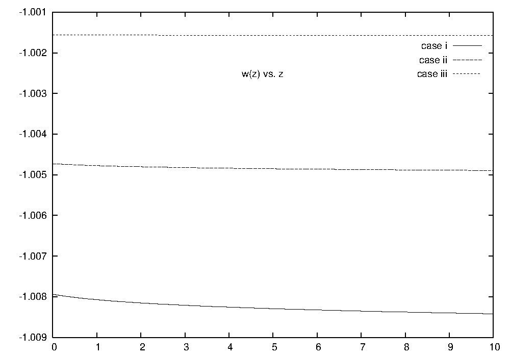
Figure 1: The Equation of State w(z)  vs. the redshift z for the three cases explicitly calculated in this paper : (i) [full line] No neutrino contribution to the dark energy and the scalar mass $M=3.96$ meV.   (ii) [broken line] A Majorana neutrino with mass $m=3.2$ meV and the scalar mass $M=4.35$ meV.   (iii) [dotted line] A Dirac neutrino with mass $m=3.2$ meV and the scalar mass $M=4.66$ meV. [See the discussion in Section IX].   In all three cases $w<-1$ by less than $1\%$.

• In Fig. 1 we plot the equation of state w(z) as a function of z for the three cases explicitly calculated in this paper:

• (i) No neutrino contribution to the dark energy and the scalar mass $M=3.96$ meV.

• (ii) A Majorana neutrino with mass $m=3.2$ meV and the scalar mass $M=4.35$ meV.

• (iii) A Dirac neutrino with mass $m=3.2$ meV and the scalar mass $M=4.66$ meV. [See the discussion in Section IX].

• We see that the equation of state in all the three cases (i)-(iii) differs from the cosmological constant case $w=-1$ by less than $1\%$.

• The value of the lightest neutrino mass Eq.(138) is well below the neutrino mass splittings $\sqrt{\Delta m^{2}_{sun}}$ and $\sqrt{\Delta m^{2}_{atm}}$ and consistent with both direct and inverse mass hierarchies. A quasi-degenerate mass spectrum will give a large negative contribution to the dark energy and will require a scalar particle with a mass $M\gtrsim 100$ meV to reproduce the observed dark energy data Eq.(123). Such a particle can very well exist but it cannot be the axion [see Eq.(127)]. Indeed, the scalar particle can have the mass value given by Eq.(140) in case all three neutrinos decay in a time scale of the age of the universe in order to dissipate their cosmological vacuum energy as discussed in Section VIII.

• On the other hand, a range of neutrino masses from $10^{-3}$ eV to $0.1$ eV in agreement with neutrino mass differences from oscillations and the value Eq.(138) for the mass of the lightest neutrinos is compatible with a consistent baryogenesis.

XII Conclusions

• We find that the presence of a cosmological quantum vacuum energy with an equation of state just below $-1$ is the unavoidable consequence of the existence of light particles with very weak couplings. Bosons yield positive contributions and fermions yield negative contributions to the vacuum energy.

• It must be noticed the present lack of knowledge about the low energy (energy $\sim 1$ meV) particle physics region. Actually, most of the constraints on this sector follow from astrophysics and cosmology including the new constraints that we obtain here on the axion mass.

• No exotic physics needs to be invoked to explain the dark energy. Since the observed energy scale of the dark energy is very low, we find natural to explain it only through low energy physics. The effects from energy scales higher than 1 eV or even 1 MeV arrive strongly suppressed to the dark energy scale of 1 meV.

• In summary, dark energy can be explained by a very light and very weakly coupled scalar particle which decouples by redshift $z_{S}\gg 1$. If the scalar particle is the axion, then $z_{S}\sim 2.2\times 10^{18}$.

  We have four main cases:

• (i) No neutrino contribution. This happens when the lightest neutrino has a mass $m\ll 1$ meV and when the vacuum neutrino contribution dissipates in the time scale of the age of the universe [see Eq.(133)]. The scalar mass must be

  $$M\;=\;\frac{10.1\;{\rm meV}}{\left(\;\log z_{S}\;-\;\frac{1}{4}\;\right)^{\!\frac{1}{4}}}\quad:\quad{\rm no~{}vacuum~{}neutrino~{}energy}\;.$$ (151)

  If the scalar is the axion, then $M=3.96$ meV in this case.

• (ii) The lightest neutrino is Majorana and has a mass $m\simeq 3.2$ meV. Then, the scalar mass must be

  $$M\;=\;\frac{11.1\;{\rm meV}}{\left(\;\log z_{S}\;-\;\frac{1}{4}\;\right)^{\!\frac{1}{4}}}\quad:\quad{\rm the~{}Majorana~{}neutrino~{}contributes}$$

  If the scalar is the axion, then $M=4.35$ meV in this case.

• (iii) The lightest neutrino is Dirac and has a mass $m\simeq 3.2$ meV. Then, the scalar mass must be

  $$M\;=\;\frac{11.9\;{\rm meV}}{\left(\;\log z_{S}\;-\;\frac{1}{4}\;\right)^{\!\frac{1}{4}}}\quad:\quad{\rm the~{}Dirac~{}neutrino~{}contributes}$$

  If the scalar is the axion, then $M=4.66$ meV in this case.

• Therefore, in all the three cases (i)-(iii) above where the axion explains the dark energy we predict its mass in the range:

  $$3.96\;{\rm meV}\;<M\;<\;4.66\;{\rm meV}\;.$$ (152)

  The left and right ends of the interval in Eq.(152) correspond to no neutrino contribution and to the lightest neutrino as a Dirac fermion with mass $m=3.2$ meV, respectively.

• In short, we uncovered here the general mechanism producing the dark energy today. This mechanism has it grounds on well known quantum physics and cosmology. The dark energy appears as a quantum vacuum effect arising when stable and weakly coupled quantum fields live in expanding cosmological space-times. That is to say, dark energy in the universe today is a QFT effect in (classical) curved space-times. That is to say, this is a semiclassical gravity effect.

• In addition, we have found here that the axion with mass in the meV range is a very serious candidate for dark energy, while we have shown already HdVNSaxion , UniversekeV that it is robustely excluded as a dark matter candidate. The cosmic dark energy today is in the meV scale while the dark matter (cosmic and galactic) particle is in the keV scale HdVNSkeV , UniversekeV .

• Many research avenues open now connecting dark energy and light particles physics. The more immediate being:

• (1) The study of the radiative corrections to the axion and neutrino cosmological vacuum evolution from their interactions.

• (2) The study of the early neutrino and axion dynamics at temperatures $\gtrsim 1$ MeV and $\gtrsim 10^{6}$ GeV, respectively.

• (3) The study of particle propagation in the media formed by the axion and the neutrino vacuum.

• (4) Last but not least: The probable deep connection between dark energy and dark matter through low energy particle states beyond the Standard Model of particle physics.

Appendix A Dimensional and Cutoff Regularization of the Vacuum Energy

Physical vacuum quantities are computed in Section IV as the equal point limit of two point functions. The distance $z$ between the points Eq.(90) naturally plays the role of the regularization parameter. Alternatively, one can regularize the two point function with dimensional regularization or cutoff regularization and set $z=0$ in the regularized expressions.

In dimensional regularization, we have

$$G_{\epsilon}(M\,a,a)\;\equiv\;<T\;\varphi({\vec{x}},\eta)\;\varphi({\vec{x}},\eta)>\;=\;\frac{1}{a^{2}}\;\int\frac{d^{4-2\,\epsilon}k}{(2\,\pi)^{4-2\,\epsilon}}\;\;\frac{i}{k^{2}-a^{2}\;M^{2}+i\,0}$$ (153)

$$\;=\;\frac{M^{2-2\,\epsilon}}{(4\,\pi)^{2-\epsilon}}\;\;\frac{1}{a^{2\,\epsilon}}\;\;\Gamma(\epsilon-1)\;.$$ (154)

Subtracting the value in Minkowski space-time ($a=1$) yields,

$$G_{\epsilon}(M\,a,a)-G_{\epsilon}(M,1)\;=\;M^{(2-2\;\epsilon)}\;\;\frac{\Gamma(\epsilon-1)}{(4\,\pi)^{(2-\epsilon)}}\;\left[\,a^{-2\,\epsilon}-1\,\right]\;\buildrel\epsilon\to 0\over{=}\;\frac{M^{2}}{2\,(2\,\pi)^{2}}\;\log a$$ (155)

in agreement with Eq.(97).

Alternatively, by regularizing with an ultraviolet cutoff $\Lambda$ in four space-time dimensions, we have

$$G_{\Lambda}(M\,a)\;\equiv\;\frac{1}{a^{2}}\;\int\frac{d^{4}k}{(2\,\pi)^{4}}\;\frac{i}{k^{2}-a^{2}\;M^{2}+i\,0}\;=\;\left(\frac{\Lambda}{4\,\pi\;a}\right)^{2}-\left(\frac{M}{4\,\pi}\right)^{2}\;\log\left[1+\left(\frac{\Lambda}{M\;a}\right)^{2}\right]=$$ (156)

(157)

$$\buildrel\Lambda\to\infty\over{=}\left(\frac{\Lambda}{4\,\pi\;a}\right)^{2}-\frac{M^{2}}{2\,(2\,\pi)^{2}}\;\log\left[\,\frac{\Lambda}{M\;a}\,\right]\;.$$ (158)

Subtracting the divergence in $\Lambda=\infty$ again leads to the result Eqs. (155) and (97):

$$G_{\Lambda}(M\,a)-\left[\left(\frac{\Lambda}{4\,\pi\;a}\right)^{2}-\frac{M^{2}}{2\,(2\,\pi)^{2}}\;\log\frac{\Lambda}{M}\right]\;\buildrel\Lambda\to\infty\over{=}\;\frac{M^{2}}{2\,(2\,\pi)^{2}}\;\log a\;.$$

We have therefore verified that the point splitting regularization used in Section IV as well as dimensional and cutoff regularization methods yield identical results. (It is known since longtime that dimensional regularization gives the same physical results than other regularization methods lapluta ). Analogous results are valid for the two point fermion function.

Acknowledgment: We thank Daniel Boyanovsky, P. Astier, G. Smoot, S. Perlmutter, B. Schmidt and A. Riess for useful discussions, and Carlos Frenk for interesting correspondence.

References

- (1) A. G. Riess et al., Astron. J. 116, 1009 (1998). P. Garnavich et al., Astrophys. J. 509, 74 (1998). S. Perlmutter et al., Astrophys. J. 517, 565 (1999).
- (2) B. P. Schmidt, Measuring global curvature and Cosmic acceleration with Supernovae, in ”Phase Transitions in Cosmology: Theory and Observations” NATO ASI Series vol 40, pp 249-266, Eds H. J. de Vega, I. M. Khalatnikov and N. G. Sanchez, Kluwer Publ (2001).
- (3) R.A. Knop et al., Astrophys. J. 598, 102 (2003). A. G. Riess et al., Astrophys. J. 607, 665 (2004). Supernova Cosmology Project homepage: http://panisse.lbl.gov/ P. Astier et al., Astron. Astrophys. 447, 31 (2006). Supernova Legacy Survey homepage: http://www.cfht.hawaii.edu/SNLS/
- (4) D. J. Eisenstein et al., Astrophys. J. 633, 560 (2005). A. Conley et al., Astrophys. J. 644, 1 (2006). W. M. Wood-Vasey et al. Astrophys. J. 666 694-715 (2007). G. Miknaitis et al. Astrophys. 666, 674-693 (2007). A. G. Riess et al., Astrophys.J. 659, 98-121 (2007).
- (5) T. Abbott, F.B. Abdalla, et al., MNRAS, 460, 1270 (2016). T.M.C. Abbott, S. Allam et al, ApJ Letters, 872, 2, L30, (2019). T. M. C. Abbott, M. Aguena, A. Alarcon, S. Allam, O. Alves, A. Amon, et al, Phys. Rev. D 105, 023520 (2022).
- (6) Euclid https://sci.esa.int/web/euclid/
- (7) Legacy Survey of Space and Time LSST-Vera C. Rubin Observatory https://www.lsst.org/
- (8) P. J. E. Peebles, B. Ratra, Revs. Mods. Phys. 75, 559 (2003). T. Padmanabhan, Phys. Rept. 380, 235 (2003). E. J. Copeland, M. Sami, S. Tsujikawa, Int. J. Mod. Phys. D15, 1753-1936 (2006). S. Nobbenhuis, Found. Phys. 36, 613,(2006) and references therein. J. A. Frieman, M. S. Turner, D. Huterer, Annual Review of Astronomy and Astrophysics Vol 46: 385-432 (2008). D. Huterer, D. L. Shafer, Rep. Prog. Phys. 81, 016901 (2018).
- (9) R. Fardon, A. E. Nelson, N. Weiner, JCAP 0410: 005 (2004) and JHEP 0603: 042 (2006) . R. D. Peccei, Phys. Rev. D71, 023527 (2005). P. Q. Hung, hep-ph/0010126. R. Horvat, JCAP 0601: 015 (2006). S. Das, N. Weiner, Phys. Rev. D 84, 123511 (2011). E. I. Guendelman, A. B. Kaganovich, Phys. Rev. D87, 044021 (2013). E. Di Valentino, S. Gariazzo, O. Mena, S. Vagnozzi JCAP 2007,045 (2020).
- (10) M. J. Mortonson, D. H. Weinberg, M. White, http://pdg.lbl.gov, Particle Data Group Review of Particle Physics, 25 (2014). N. Frusciante, L. Perenon, Phys. Rept. 85, 1-63 (2020). J. Sola Peracaula, Phil. Trans. R. Soc. A 380, 20210182 (2022).
- (11) A. Albrecht, G. Bernstein, R. Cahn, W. L. Freedman, J. Hewitt et al, arXiv:astro-ph/0609591, Report of the Dark Energy Task Force, DoE, NASA and NSF, (2006), .
- (12) J. Frieman, M. Turner, D. Huterer, Ann. Rev. Astron. Astrophys. 46: 385-432, (2008).
- (13) Adam G. Riess et al, The Astrophysical Journal 876: 85 (2019).
- (14) Adam G. Riess et al, The Astrophysical Journal Letters, 908: L6, (2021). Adam G. Riess et al,The Astrophysical Journal Letters, 934: L7, (2022); Astrophys.J. 938, 1, 36 (2022).
-
(15)
The Award, Surprises in the Expansion History of the Universe:
https://chalonge-devega.fr/Riess-07Dec22.mp4 - (16) N. Aghanim, Y. Akrami, M. Ashdown, J. Aumont, C. Baccigalupi et al, Astron.Astrophys. 641 (2020) A6, Astron.Astrophys. 652 (2021) C4 (erratum), e-Print: 1807.06209 [astro-ph.CO].
- (17) E. Abdalla, G. Franco Abellan, A. Aboubrahim, A. Agnello, O. Akarsu et al. , arXiv:2203.06142, 2022 Snowmass Summer Study, 49-211 (2022), J. High En. Astrophys. 2204, 002 (2022).
- (18) N. G. Sanchez, Phys. Rev. D 104, 123517 (2021).
- (19) N. G. Sanchez, Int. J. Mod Phys A34, 1950155 (2019).
- (20) N.G. Sanchez, Int. J. Mod Phys D28, 1950055 (2019).
- (21) D. Boyanovsky, H. J. de Vega, R. Holman, D S Lee and A Singh, Phys. Rev. D51, 4419 (1995). D. Boyanovsky, H. J. de Vega, R. Holman and J. F. J. Salgado, Phys. Rev. D54, 7570 (1996) and Phys. Rev. D59, 125009 (1999).
- (22) D. Boyanovsky, M. D’Attanasio, H.J. de Vega, R. Holman, and D.-S. Lee, Phys. Rev. D52, 6805 (1995).
- (23) J. Baacke, C. Pätzold, Phys. Rev. D62, 084008 (2000).
- (24) D. Boyanovsky, C. Destri, H. J. de Vega, R. Holman, J. F. J. Salgado, Phys. Rev. D57, 7388 (1998).
- (25) W. M. Yao et al. J. Phys. G33, 1 (2006), PDG WWW pages http://pdg.lbl.gov/. D. N. Spergel et al, Astrophys. J. Suppl. 170, 377 (2007). N. Aghanim et al. Astronomy & Astrophysics 641: A6 (2020). T. M. C. Abbott, M. Aguena, A. Alarcon, S. Allam, O. Alves, A. Amon, et al, Phys. Rev. D 105, 023520 (2022).
- (26) R. D. Peccei and H. R. Quinn, Phys. Rev. Lett 38, 1440 (1977), Phys. Rev. D16, 1791 (1977). S. Weinberg, Phys. Rev. Lett 40, 223 (1978); F. Wilczek, Phys. Rev. Lett. 40, 279 (1978). R. T. Co, L. J. Hall, K. Harigaya, Phys. Rev. Lett. 124, 251802 (2020).
- (27) J. E. Kim, Phys. Rev. Lett. 43, 103 (1979). M. A. Shifman, A. I. Vainshtein, and V. I. Zakharov, Nucl. Phys. B166, 493 (1980). M. Dine, W. Fischler and M. Srednicki, Phys. Lett. B104, 199 (1981). A. R. Zhitnitsky, Sov. J. Nucl. Phys. 31, 260 (1980). J. E. Kim, G. Carosi, Rev. Mod. Phys. 82, 557-602, (2010) and Rev. Mod. Phys. 91, 049902 (2019).
- (28) Y. Chikashige, R. N. Mohapatra, R. D. Peccei, Phys. Lett. B 98, 265 (1981) and Phys. Rev. Lett. 45, 1926 (1980).
- (29) S. Dodelson, Modern Cosmology, Academic Press, San Diego, (2003).
- (30) E. W. Kolb and M. S. Turner, ‘The Early Universe’, Addison Wesley, Redwood City, CA, (1990).
- (31) D. S. Gorbunov, V. A. Rubakov, Theory of the Early Universe I, Hot Big Bang Theory, World Scientific, Singapore (2011). ”Neutrino 2022” virtual Seoul, 50th Anniversary, Neutrino results, 30 May - 4 June (2022).
- (32) E. Di Valentino, A. Melchiorri, O. Mena, JCAP 11, 018 (2013). M. Archidiacono, S. Gariazzo, Universe 2022, 8(3), 175; https://doi.org/10.3390/universe8030175 (2022).
- (33) R. D. Peccei, Lect. Notes Phys. 741, 3-17 (2008). P. Sikivie, Lect. Notes Phys. 741, 19-50 (2008). D.J.E Marsh, Phys. Rep. 643, 1-79 (2016). S. S. Borsanyi et al, Phys. Lett. B 752, 175 (2016). G. Ballesteros, Phys. Rev. Lett. 118, 071802 (2017).
- (34) C. Balazs, S. Bloor, T. E. Gonzalo, W. Handley, S. Hoof et al , JCAP 12, 027 (2022).
- (35) R. Hlozek, D. Grin, D.J.E. Marsh, P. G. Ferreira, Phys. Rev. D 91, 10, 103512 (2015).
- (36) A. Sirlin, Comm. Nucl. Part. Phys. 21, 227 (1994). See also Ref. masanu2 .
- (37) C. H. Albright, Phys. Lett. B 599: 285 (2004).
- (38) See for example, J. A. Casas et al. JHEP 0704, 064 (2007). W-L Guo, Int. J. Mod. Phys. E16, 1-50 (2007).
- (39) G. G. Raffelt, Lect. Notes Phys. 741, 51-71 (2008). W. Keil et al, Phys. Rev. D56, 2419 (1997). H-T Janka et al. Phys. Rev. Lett. 76, 2621 (1996). ”Neutrino 2022” virtual Seoul, 50th Anniversary, Neutrino Mass results, 30 May - 4 June (2022).
- (40) P. Sikivie, Q. Yang, Phys. Rev. Lett. 103, 111301 (2009). O. Erken et al. Phys. Rev. D85, 063520 (2012). P. Sikivie, Lect. Notes Phys. 741, 19-50 (2008) . N. Crisosto, P. Sikivie et al., Phys. Rev. Lett. 124, 241101 (2020).
- (41) N. D. Birrell, P. C. W. Davies, Quantum fields in curved space, Cambridge Monographs in Mathematical Physics, Cambridge University Press, Cambridge, (1982).
- (42) D. Boyanovsky, H. J. de Vega, N. G. Sanchez, Phys. Rev. D 72, 103006 (2005) and references therein.
- (43) C. Itzykson, J B Zuber, Quantum Field Theory, McGraw-Hill, New York, 1980.
- (44) Table of Integrals, Series and Products, I. S. Gradshteyn and I. M. Ryzhik, Academic Press, New York, 1965.
- (45) J. W. F Valle, Prog. Part. Nucl. Phys. 26, 91 (1991), AIP Conf. Proc. 878, 369-384 (2006) and Nucl. Phys. Proc. Suppl. 168, 413-422 (2007). J. Lesgourgues, S. Pastor, Phys. Rept. 429, 307 (2006). R. N. Mohapatra, A. Y. Smirnov, Annu. Rev. Nucl. Part. Sci. 56, 569 (2006). S. Hannestad, Annu. Rev. Nucl. Part. Sci. 56, 137 (2006).
- (46) M. S. Turner, Phys. Rev. Lett 59, 2489 (1987) and 60, 1101(E) (1987). E. Massó, F. Rota, G. Zsembinszki, Phys. Rev. D66, 023004 (2002).
- (47) Z.Chacko, L. J. Hall, T. Okui, S. J. Oliver, Phys.Rev. D70, 085008 (2004). Z. Chacko, L. J. Hall, S. J. Oliver, M. Perelstein, Phys. Rev. Lett. 94, 111801 (2005). T. Okui, JHEP 0509, 017 (2005). L. J. Hall, S. J. Oliver, Nucl. Phys. Proc. Suppl. 137, 269, (2004). H. Davoudiasl, R. Kitano, G. D. Kribs, H. Murayama, Phys. Rev. D71, 113004 (2005). C. Boehm, Y. Farzan, T. Hambye, S. Palomares-Ruiz, S. Pascoli, Phys. Rev. D77, 043516 (2008). N. F. Bell, E. Pierpaoli, K. Sigurdson, Phys. Rev. D73, 063523 (2006). Y. Farzan, Phys. Rev. D67, 073015 (2003). J. L. Baker, H. Goldberg, G. Perez, I. Sarcevic, Phys. Rev. D76, 063004 (2007). H. Goldberg, G. Perez, I. Sarcevic, JHEP 0611, 023 (2006).
- (48) M. Markevitch et al., ApJ, 606, 819 (2004).
- (49) This value follows by setting (neutrinos has no charge) in Eq.(1) of Ref. masanu . We thank Alberto Sirlin for calling our attention on this point.
- (50) D. Boyanovsky, H. J. de Vega, R. Holman, Phys. Rev. D49, 2769 (1994).
- (51) D. Boyanovsky, H. J. de Vega, N. G. Sanchez, Phys. Rev. D74, 123006 (2006) and Phys. Rev. D74, 123007 (2006). C. Cao, H. J. de Vega, N. G. Sanchez, Phys. Rev. D78, 083508 (2008). C. Destri, H. J. de Vega, N. G. Sanchez, Phys. Rev. D78, 023013 (2008) and Phys. Rev. D81, 063520 (2010).
- (52) A. R. Liddle, P. Mukherjee, D. Parkinson, Y. Wang, Phys. Rev. D74, 123506 (2006). D. Huterer, A. Cooray, Phys. Rev. D71, 023506 (2005). U. Alam, V. Sahni, A. A. Starobinsky, JCAP 0406 008 (2004) and JCAP 0702, 011 (2007). H. Ziaeepour, Mod. Phys. Lett. A22: 1569-1580, (2007). Y. Gong, A. Wang, Phys. Rev. D75, 043520 (2007).
- (53) U. Seljak, A. Slosar, P. Mc Donald, JCAP 0610, 014 (2006).
-
(54)
H. J. de Vega, N. G. Sanchez,
Universe 2022, 8(8), 419,
https://doi.org/10.3390/universe8080419 - (55) H. J. de Vega, N. G. Sanchez, Mon. Not. Roy. Astron. Soc. 404, 885 (2010). H. J. de Vega, N. G. Sanchez, Eur. Phys. J. C 77, 81 (2017). C. Destri, H. J. de Vega, N. G. Sanchez, Astrop. Phys. 46, 14 (2013). H.J. de Vega, N.G. Sanchez, Phys. Rev. D 2012, 85, 043516 and 043517. C. Destri, H.J. de Vega, N. G. Sanchez, Phys. Rev. D 201 88, 083512 (2013). H. J. de Vega, P. Salucci, N. G. Sanchez, Mon. Not. Roy. Astron. Soc. 442, 2717 (2014). H. J. de Vega, N. G. Sanchez, Universe 2022, 8, 154, https://www.mdpi.com/2218-1997/8/3/154
-
(56)
Universe, Special
Issue keV Warm Dark Matter in Agreement
with Observations in Tribute to Hector de
Vega, 2021 and the Papers Therein, 2021, 7 and 2022, 8. Available online:
https://www.mdpi.com/journal/universe/special_issues/kWDM (accessed on 28 May 2022). - (57) B. P. Abbott et al. (The LIGO Scientific Collaboration and the Virgo Collaboration) Phys. Rev. D 100, 104036 (2019).
- (58) C. G. Bollini, J. J. Giambiagi, Nuovo Cim. B12, 20 (1972). Phys. Lett. B40, 566 (1972). G. ’t Hooft, M. Veltman, Nucl. Phys. B44, 189 (1972). H J de Vega, F. A. Schaposnik, J. of Math. Phys. 15, 1998 (1974).