Photodissociation feedback of Population III stars
on their neighbor prestellar cores

Abstract

We investigate the star formation process in primordial environment in the presence of radiative feedback by other population III stars formed earlier. In this paper, we focus our attention on the effects by photodissociative radiation toward the full understanding of the radiative feedback effects. We perform three dimensional radiation hydrodynamics simulations on this issue as well as analytic estimates, paying special attention on the self-shielding effect and dynamics of the star-forming cloud. As a result, we find that the ignition timing of the source star is crucial. If the ignition is later than the epoch when the central density of the collapsing cloud exceeds $\sim 10^{3}-10^{4}{\rm cm^{-3}}$, the collapse cannot be reverted, even if the source star is located at $\lesssim$ 100pc. The uncertainty of the critical density comes from the variety of initial conditions of the collapsing cloud. We also find the analytic criteria for a cloud to collapse with given central density, temperature and the Lyman-Werner(LW) band flux which irradiates the cloud. Although we focus on the radiation from neighbor stars, this result can also be applied to the effects of diffuse LW radiation field, that is expected to be built up prior to the reionization of the universe. We find that self-gravitating clouds can easily self-shield from diffuse LW radiation and continue their collapse for densities larger than $\sim 10^{3}{\rm cm^{-3}}$.

1 Introduction

One of the important objectives of cosmology today is to understand the way how the first generation stars or galaxies are formed and how they affected the later structure formation, and how they reionize the surrounding media. In particular, the self-regulation of star formation in the first low mass halos is quite important, since it controls the Population III (POPIII) star formation activity in the early universe, which is the key for the reionization and the metal pollution of the universe. These problems have been studied intensively in the last decade, hence we already have some knowledge on these issues (see review by Bromm & Larson 2004). However, studies which properly address the radiation transfer effects are still at the beginning, in spite of their great importance.

Radiation from the first generation stars play quite important roles on the formation of stars/galaxies through two main physical processes. Since first stars are expected to be very massive (Omukai & Nishi, 1998; Abel, Bryan, Norman, 2000; Bromm, Coppi & Larson, 2002; Nakamura & Umemura, 1999, 2001), the amount of ultraviolet photons are quite large. Once these kinds of stars are formed, 1) emitted Lyman-Werner (LW) band photons photodissociate the hydrogen molecules in the neighborhood by Solomon process(Hiaman, Rees & Loeb, 1997; Omukai & Nishi, 1999; Glover & Brand, 2001; Machacek, Bryan & Abel, 2001). Afterwards or simultaneously 2) ionizing photons propagate into surrounding media, followed by the photoionization and heating of the gas. Since hydrogen molecules are the only coolant in low mass first generation objects, and the photoheated gas is too hot to be kept in such small dark halos, these radiative feedbacks are basically expected to have negative effects on the structure formation (e.g. Susa & Umemura 2004ab). In contrast, enhanced fraction of electrons by photoionization can lead to efficient H₂ formation (Shapiro & Kang, 1987; Kang & Shapiro, 1992; Susa et al., 1998; Oh & Haiman, 2002), and it could accelerate the structure formation (Ricotti, Gnedin, & Shull, 2001; O’shea, Abel, Whalen & Norman, 2005; Nagakura & Omukai, 2005; Susa & Umemura, 2006; Ahn & Shapiro, 2006; Yoshida et al., 2006).

Since these physical processes related to this issue are so complicated, we try to understand one by one. In this paper, we focus our attention on the photodissociation feedback effect including the effect of self-shielding. We do not take into account the effects by photoionization, which is discussed with limited parameters in Susa & Umemura (2006), and will be presented in detail in the forthcoming paper.

Concerning the photodissociation feedback effects, there are two contexts. First one is the local feedback by the nearby POPIII stars formed in the same halo or in the neighbor halos. Another one is the feedback by diffuse LW background radiation, that is built up by the formed POPIII stars in many dark halos spread in the universe(Machacek, Bryan & Abel, 2001; Yoshida et al., 2003). In reality, the former would particularly be important at the early phase of the POPIII star formation episode, ahead of the latter effect. Local feedback might also play important roles in the star formation process in relatively larger halos whose virial temperature is higher than $10^{4}$K. The physical difference of the two cases are the different duration and intensity of radiation field. In the latter case, intensity is not so high, whereas the radiation field irradiate the halos continuously since it is a background. In contrast, in the former case, the radiation source basically turn-off after the life-time of the source star, although the intensity of the radiation could be much higher than the diffuse background. In this paper, we mainly investigate the local effects.

Omukai & Nishi (1999) investigated on this issue in an uniform virialized halo. They argue that only a single massive POPIII star can destroy H₂ molecules within $\sim 1$kpc, which is comparable to the virial radius of $10^{8}M_{\odot}$ halos at $z\gtrsim 10$. This means that star formation in such low mass halos is highly regulated by themselves. On the other hand, Glover & Brand (2001) considered more realistic clumpy halos. They simply assessed the photodissociation time scale and free-fall time of the dense clouds. Comparing these two time scales, they found that if the gas density is sufficiently high, dissociation time scale could be longer than the free-fall time, which allow the cloud to collapse. Although those arguments are quite clear, they are based upon very simplified configuration. Therefore, more sophisticated treatments are necessary to investigate this feedback process. In order to improve the understanding of this issue, we carry out three dimensional radiation hydrodynamics simulations as well as more detailed analytic arguments.

This paper is organized as follows: in the next section, we briefly summarize the numerical scheme employed. In §3, setup of our numerical simulations are shown. We present the numerical and analytical results in §4 and §5. §6 and §7 are devoted to discussion and summary.

2 Numerical method

We perform numerical simulations by Radiation-SPH code developed by ourselves (Susa, 2006). In this section, we try to briefly summarize the scheme. The code is designed to investigate the formation and evolution of the first generation objects at $z\gtrsim 10$, where the radiative feedback from various sources play important roles. The code can compute the fraction of chemical species e, H⁺, H, H^-, H₂, and H${}_{2}^{+}$ by fully implicit time integration. It also can deal with multiple sources of ionizing radiation, as well as the radiation at Lyman-Werner band.

Hydrodynamics is calculated by Smoothed Particle Hydrodynamics (SPH) method. We use the version of SPH by Umemura (1993) with the modification according to Steinmetz & Müller (1993). We adopt the particle resizing formalism by Thacker et al. (2000).

The non-equilibrium chemistry and radiative cooling for primordial gas are calculated by the code developed by Susa & Kitayama (2000), where H₂ cooling and reaction rates are mostly taken from Galli & Palla (1998). As for the photoionization process, we employ so-called on-the-spot approximation (Spitzer, 1978), but we do not get into the details since we do not show the results with ionizing radiation in this paper.

The optical depth is integrated utilizing the neighbour lists of SPH particles. It is similar to the code described in Susa & Umemura (2004a), but now we can deal with multiple point sources. In our new scheme, we do not create so many grid points on the light ray as the previous code Susa & Umemura (2004a) does. Instead, we just create one grid point per one SPH particle in its neighbor. We find the ’upstream’ particle for each SPH particle on its line of sight to the source. Then the optical depth from the source to the SPH particle is obtained by summing up the optical depth at the ’upstream’ particle and the differential optical depth between the two particles.

The opacity of LW radiation is calculated by utilizing the original self-shielding function(Draine & Bertoldi, 1996). The column density of H₂ is evaluated by the method described above. We assume same absorption for the photons within LW band, i.e. between 11.26eV and 13.6eV.

The code is already parallelized with MPI library. The computational domain is divided by so called Orthogonal Recursive Bisection method(Dubinski, 1996). The parallelization method for radiation transfer part is similar to Multiple Wave Front method developed by Nakamoto, Umemura, & Susa (2001) and Hieneman et al. (2005), but it is changed to fit the SPH scheme. The code also is able to handle self-gravity with Barnes-Hut tree(Barnes & Hut, 1986), which is also parallelized. The code is tested for various standard problems(Susa, 2006). We also take part in the code comparison project with other radiation hydrodynamics codes (Iliev et al., 2006) in which we find reasonable agreements with each other.

3 Setup of Numerical simulations

We simulate the collapsing primordial gas cloud with $M=8.3\times 10^{4}M_{\odot}$, which is initially uniform and spherical. The initial number density is $14{\rm cm^{-3}}$, whereas the corresponding radius is $\sim 40$pc. We employ four initial temperatures $T_{\rm ini}=50$K, $100$K , $200$K and $350$K which represent the coldness of the initial collapses. The uniform cloud is embedded in an extended uniform low density cloud with $0.1{\rm cm^{-3}}$ and the same temperature as the dense cloud. Remark that such a thin surrounding material does not affect the fate of the dense cloud. The mass of an SPH particle is $0.32M_{\odot}$. We employ 524288 particles in total. Approximetely half of the particles are used to represent the initial dense region. The chemical compositions are assumed to be the cosmological residual values (Galli & Palla, 1998).

We start numerical simulations from this initial setup without any radiative feedback effects. Then, the dense clump collapses in run-away fashion because of the self-gravity and the radiative cooling by H₂ . When the central density exceeds a certain limit, $n_{\rm on}$, we ignite a 120$M_{\odot}$ POPIII star that is located $D$ pc distant from the center of the dense clump. The luminosity and the effective temperature of the star are taken from Baraffe, Heger & Woosely (2001). We employ various parameters in the range $3\times 10^{2}{\rm cm^{-3}}\leq n_{\rm on}\leq 1\times 10^{5}{\rm cm^{-3}}$, and $20{\rm pc}\leq D\leq 200{\rm pc}$. In this paper, the ionizing photons are not included, since we focus on the photodissociation process. Simulated physical time is $10^{7}$ yr, which is significantly longer than the life time of a 120$M_{\odot}$ star ($\sim 2$Myr). During the simulation time, we do not turn-off the source star, as we are interested in both of the effects by diffuse background/local LW radiation (diffuse radiation never turns-off).

Numerical simulations are mainly carried out on parallel computer system called “FIRST” installed in University of Tsukuba. The newly being developed PC cluster “FIRST” is designed to elucidate the origin of first generation objects in the Universe through large-scale simulations. The cluster consists of 240 nodes ( each node has dual Xeon processors ). The most striking feature of the system is that each node has small GRAPE6 PCI-X board called Brade-GRAPE. The Brade-GRAPE has four GRAPE6 chips per board (thus 1/8 processors of a full board). The board has basically the same function as GRAPE-6A (Fukushige, Makino & Kawai, 2005), but it has an advantage that it can be installed in 2U server unit of PC clusters due to the short height of its heat sink.

4 Numerical Results

4.1 Simulation without radiative feedback

Before we proceed to the results with radiative feedback, we give an outline of the results without the feedback process. Since we have no LW flux in these particular runs and total mass and the initial density are fixed, the only free parameter of these calculations is the initial temperature, $T_{\rm ini}$. Fig.1 shows the snapshots of radial density distributions of the collapsing clouds with $T_{\rm ini}=100$K and $T_{\rm ini}=350$K. The snapshots are taken when the central dense regions are very close to the resolution limits. For both of the runs, the distribution roughly converges to the $\rho\propto r^{-2}$relation, which is well known as the Larson-Penston type similarity solution (Larson, 1969; Penston, 1969) for isothermal gas. Remark that the larger $T_{\rm ini}$ results in smaller size of the cloud, since higher temperature promotes faster reaction to produce H₂, which leads to efficient cooling.

Fig.2 represents the evolution of the cloud core on density v.s. temperature plane. Four tracks correspond to $T_{\rm ini}=50,100,200,350$K, respectively. Among these, the run with $T_{\rm ini}=350$K is relatively close to the physical states of the collapsing clouds at $n_{\rm N}\gtrsim 10^{3}{\rm cm^{\-3}}$, developed from the CDM density fluctuations (see figures 11,12 in O’shea & Norman 2006). The runs with $T_{\rm ini}=50,100$K also could be realized in the shock compressed layers in larger halos with $M\gtrsim 10^{8-9}M_{\odot}$ since the gas is cooled down to $\lesssim 100$K due to the efficient H₂ cooling(Shapiro & Kang, 1987; Kang & Shapiro, 1992; Susa et al., 1998; Uehara & Inutsuka, 2000). Thus, the various $T_{\rm ini}$ should be regarded as the variety of the initial conditions for the sites of primordial star formation.

4.2 Typical results with radiative feedback

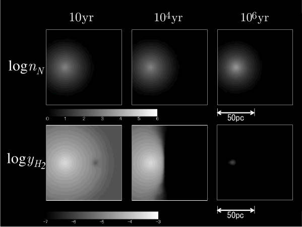
Figure 3: Time evolution of the density distribution and H₂ distribution are shown for $D=40{\rm pc}$, $n_{\rm on}=10^{3}{\rm cm^{-3}}$, $T_{\rm ini}=100{\rm K}$. Top panels represent the density distribution on the slice which include the axis of symmetry after the ignition of nearby star. Three panels correspond to $t=10$yr, $10^{4}$yr and $10^{6}$yr, respectively. Bottom panels also show the snapshots of $y_{\rm H_{2}}$ distribution at three epochs.

First, we show two typical results among various runs. Figure 3 shows the density / H₂ map on the slice that contains the axis of symmetry in the run with $T_{\rm ini}=100{\rm K},~{}n_{\rm on}=10^{3}{\rm cm^{-3}},D=40{\rm pc}$. Top panels represent three snapshots, those correspond to $t=10$yr, $10^{4}$yr and $10^{6}$yr, respectively. Bottom panels also show $y_{\rm H_{2}}$ distribution at same physical time. In this run, H₂ are totally photodissociated by the nearby star, even at the center of the collapsing cloud (lower panels). H₂ fraction never recovers through the simulation time. As a result, the cloud cannot keep collapsing because of the absence of coolants. The cloud bounces after the adiabatic compression phase.

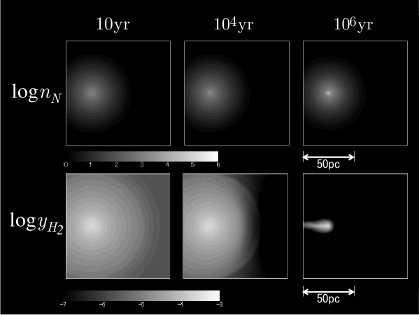
Figure 4: Same as Figure 3 except $D=100{\rm pc}$.

On the other hand, Figure 4 shows the case same as Figure 3 except $D=100$pc. Since the Lyman-Werner band flux is smaller than the previous case, H₂ is self-shielded and survive at the center (lower panels), followed by the collapse of the core (upper right panel). Figure 5 shows the time evolution of the central H₂ fraction for four models including above two. The four models correspond to $D=40,60,80,100$pc respectively, whereas other parameters $n_{\rm on}=10^{3}{\rm cm^{-3}}$ and $T_{\rm ini}=100{\rm K}$ are common. The horizontal axis shows the time after the collapse started, while the vertical axis shows the H₂ fraction at the center of the cloud. We find that H₂ molecules are photodissociated just after the ignition of the source stars for all models. After the dissociation, H₂ fraction recovers immediately. For the models with $D=80,100$pc, the recoveries are sufficient to cool the gas ($y_{\rm H2}\sim 10^{-4}$ is required), whereas it is not true for $D=40$pc case. $D=60$pc is the marginal case, in which the cloud manage to collapse although it is delayed significantly, because the cooling time is slightly longer than the free-fall time. We will discuss this delicate behaviour of H₂ fraction in section 5.2.

4.3 Summary of numerical runs

Figure 6 shows the results of various runs. Four panels correspond to $T_{\rm ini}=50,100,200,350$K, respectively. Horizontal axes represents the turn-on density $n_{\rm on}$ and vertical axes show the distance between the source star and the cloud center, $D$. Each symbol in the panels corresponds to each run. In the runs denoted by vertices, the clouds cannot collapse until the end of the simulation, i.e. $10^{7}$yr after the ignition of the source star. On the other hand, the open circles represent the runs with successful collapse. Here “collapsed cloud” is defined as the one whose central density exceeds the numerical resolution limit determined by the Jeans condition. The nominal density correspond to the resolution limit is $\sim 10^{6}-10^{7}{\rm cm^{-3}}$ in the present paper.

The results depend upon the initial temperature $T_{\rm ini}$ i.e. initial coldness of the collapsing cloud. Initially colder gas can collapse for wider range of parameters than those in hotter initial conditions. In fact, considering the case with $T_{\rm ini}=350$K (lower left panel), which is close to the prestellar core formed directly from CDM density perturbations, LW feedback is inefficient for $n_{\rm N}\gtrsim 10^{4}{\rm cm^{-3}}$ for $D\lesssim 50{\rm pc}$. Thus LW feedback from the stars in the same halo would not be effective for such dense self-gravitating cores, since the virial radius of the $\sim 10^{6}M_{\odot}$ halos at $z\sim 20-30$ is several ten parsec.

On the other hand, considering $T_{\rm ini}=50,100$K cases, LW feedback is also ineffective (upper panels) even in less dense clouds ($n_{\rm N}\gtrsim 10^{3}{\rm cm^{-3}}$). Thus, if we regard these as the stars formed from the shocked layers or fossil HII regions, such POPII.5 stars(Jhonson & Bromm, 2006; Grief & Bromm, 2006) would not be affected by LW radiation even if the source stars are in the same halo.

These results are discussed physically in detail in the next section.

4.4 Effects of diffuse LW flux on dense cores

Before we move on to the detailed physical arguments, we evaluate the effects of diffuse LW radiation field on the primordial star formation. Previous analysis on this issue is basically based upon the optically thin approximation (e.g. Machacek, Bryan & Abel 2001), which is only valid for low density clouds. Yoshida et al. (2003) also address this issue including the effects of self-shielding in their cosmological simulations, although in an approximated manner. Present calculation can give a better understanding on this issue especially for dense clumps.

The intensity of the diffuse LW radiation background formed after the first generation stars, is expected to be $J_{\rm LW}\lesssim 10^{-21}{\rm erg/s/Hz/cm^{2}/str}$ for $z>20$ (Ciardi, Ferrara & Abel, 2000; Meisinger, Bryan, & Haiman, 2006). If we interpret this intensity as the flux from distant 120$M_{\odot}$ single POPIII star, the distance $D$ should satisfy $D\gtrsim 1{\rm kpc}$.

In view of the numerical results in Figure 6, diffuse radiation field cannot prevent the self-gravitating prestellar cores ($n_{\rm N}\gtrsim 10^{3}{\rm cm^{-3}}$) from collapsing, although the diffuse field keep irradiating the cloud more than two million years. However, it would be possible to stop the collapse at much lower density, at which the clouds are not expected to be self-gravitating (e.g. Ahn & Shapiro 2006). In such phase, dark matter gravitational force dominates the contraction, which is not included in the present paper. It is beyond the scope of our present calculations.

5 Analytic estimation

In this section, we describe the analytic collapse criteria in the presence of photodissociative feedback by a nearby star. The collapse criteria should be $t_{\rm cool}<t_{\rm ff}$, i.e. the cloud is cooled faster than it shrinks by gravity. After some algebra, an analytic expression for $t_{\rm cool}<t_{\rm ff}$ is derived, which is compared with numerical results. We also compare the derived cooling condition with $t_{\rm dis}>t_{\rm ff}$.

5.1 Non-equilibrium fraction of electrons

In order to assess the cooling time, we need the number density of hydrogen molecules. The amount of hydrogen molecules strongly depends on the electron abundance, since they are mainly formed through following reactions:

$${\rm H}+{\rm e}^{-} \rightarrow {\rm H}^{-}+h\nu$$ (1)

$${\rm H^{-}}+{\rm H} \rightarrow {\rm H}_{2}+{\rm e}^{-}$$

Thus, we also have to assess the amount of electrons, which is out of equilibrium. The fraction of electrons ($y_{\rm e}$) at the center of the collapsing cloud is not in chemical equilibrium, which follows the following rate equation:

$$\frac{dy_{\rm e}}{dt}=-k_{\rm rec}n_{\rm N}y_{\rm e}^{2}.$$ (2)

Here the collisional ionization term is omitted, because the temperature of the core is much lower than $10^{4}$ K above which the collisional ionization becomes important. Since the central part of the core collapses with free-fall time, the evolution of the hydrogen nucleon number density $n_{\rm N}$ is described as,

$$\frac{1}{n_{\rm N}}\frac{dn_{\rm N}}{dt}\simeq\left(\frac{3\pi}{32Gm_{\rm p}n_{\rm N}}\right)^{-1/2}$$ (3)

Combining above two equations, we have

$$\frac{dy_{\rm e}}{dn_{\rm N}}\simeq-n_{\rm N}^{-1/2}y_{\rm e}^{2}k_{\rm rec}\sqrt{\frac{3\pi}{32Gm_{\rm p}}}.$$ (4)

$k_{\rm rec}$ is a function of time, because it depends on the temperature ($\propto T^{-1/2}$). However, the change of temperature is not so significant during the collapse, whereas the density gets larger by several orders of magnitude. Thus, we can approximate the recombination rate $k_{\rm rec}$ as a constant when we integrate the equation (4). The equation (4) has an analytic solution:

$$y_{\rm e}=\frac{1}{y_{\rm e0}^{-1}+2\left(\sqrt{n_{\rm N}}-\sqrt{n_{\rm N0}}\right)k_{\rm rec}\sqrt{\frac{3\pi}{32Gm_{\rm p}}}},$$ (5)

where $y_{\rm e0}$ denotes the initial electron fraction, and $n_{\rm N0}$ denotes the initial number density of hydrogen nucleus. Consequently, we obtain the expression of $y_{\rm e}$ as a function of number density $n_{\rm N}$. The asymptotic behaviour of the solution (5) for $n_{\rm N}\gg n_{\rm N0}$ is

$$y_{\rm e}\simeq\frac{1}{\sqrt{n_{\rm N}}}\frac{1}{k_{\rm rec}}\sqrt{\frac{32Gm_{\rm p}}{3\pi}}.$$ (6)

This expression is independent of initial abundance $y_{\rm e0}$ and initial density $n_{\rm N0}$, except that $y_{\rm e}$ cannot exceed $y_{\rm e0}$ since we neglect the ionization processes. In fact, $y_{\rm e}$ given in equation (5) are plotted for various initial conditions $(n_{\rm N0},y_{\rm e0})$ in Figure 7. We find rapid convergences of electron fractions to equation (6) as the collapse of the clouds proceed. Therefore, as far as we consider $n_{\rm N}\gtrsim 10^{3}{\rm cm^{-3}}$, we can safely assess the electron fraction by equation (6).

5.2 H₂ abundance

Because of the intense LW radiation, H₂ at the center of the cloud is basically in chemical equilibrium with given $y_{\rm e}$. Therefore we assess the H₂ fraction $y_{\rm H_{2}}$ assuming chemical equilibrium. Equating the formation rate of H₂ and the photodissociation rate, we have

$$y_{\rm H_{2}}=\frac{n_{\rm N}y_{\rm e}k_{\rm H^{-}}}{k_{\rm 2step}}$$ (7)

where $k_{\rm H^{-}}$ denotes the reaction rate of reaction(1), $k_{\rm 2step}$ is photodissociation rate by Solomon process. These rates are

$$k_{\rm H^{-}} = 1.0\times 10^{-18}T{\rm cm^{3}s^{-1}}$$ (8)

$$k_{\rm 2step} = 1.13\times 10^{8}F_{\rm LW0}f_{\rm sh}\left(\frac{N_{\rm H_{2}}}{10^{14}{\rm cm^{-2}}}\right){\rm s^{-1}},$$ (9)

where $F_{\rm LW0}$ is the LW flux from the star in the absence of shielding, $f_{\rm sh}$ denotes the self-shielding function derived by Draine & Bertoldi (1996). It is defined as

$$f_{\rm sh}(x)=\left\{\begin{array}[]{cc}1,~{}~{}~{}~{}~{}~{}~{}~{}~{}~{}~{}~{}~{}~{}x\leq 1&\\ x^{-3/4},~{}~{}~{}~{}~{}~{}~{}~{}~{}x>1&\end{array}\right.$$

$N_{\rm H_{2}}$ denotes the hydrogen column density of the collapsing core. Since the core size is approximately given by the Jeans length, $N_{\rm H_{2}}$ is given as

$$N_{\rm H_{2}}\simeq n_{\rm N}y_{\rm H_{2}}\frac{\lambda_{\rm J}}{2}=n_{\rm N}y_{\rm H_{2}}\frac{1}{2}\sqrt{\frac{\pi k_{\rm B}T}{Gm_{\rm p}^{2}n_{\rm N}}}$$ (10)

Combining equations (6)-(10), we obtain

$$y_{\rm H_{2}}=4.3 \times 10^{-5}\left(\frac{F_{\rm LW0}}{2\times 10^{-17}{\rm erg\;s^{-1}\;cm^{-2}\;Hz^{-1}}}\right)^{-4}$$ (11)

$$\times \left(\frac{n_{\rm N}}{10^{4}{\rm cm^{-3}}}\right)^{7/2}\left(\frac{T}{10^{3}{\rm K}}\right)^{11/2}$$

Thus we have obtained the formula to assess H₂ fraction with given LW flux, density and temperature . It is worth noting that $y_{\rm H_{2}}$ is quite sensitive to density and temperature. If we consider the adiabatic collapse case, the relation $y_{\rm H_{2}}\propto T^{43/4}=T^{10.75}$ is satisfied, because of the adiabatic relation $n_{\rm N}\propto T^{3/2}$. We have already found this delicate behaviour of $y_{\rm H_{2}}$ in the previous section, where the very quick recovery of H₂ fraction is found in the adiabatic collapse phase (Figure 5). Remark that this strong dependence on temperature/density holds only if the H₂ is in chemical equilibrium. The relation is not correct for the very dense regions in which the LW shielding is significant and the dissociation time scale is much longer than the free-fall time. However, H₂ fraction is large enough to cool the gas cloud in such dense regions even without such delicate behaviour.

5.3 Cooling criteria

Now we are ready to find the cooling criteria. We can evaluate the cooling time utilizing the equation (11). The cooling function around $10^{3}$K is approximated as

$$\Lambda_{\rm H_{2}}\simeq\left\{\begin{array}[]{cc}4.0\times 10^{-25}n_{\rm N}^{2}y_{\rm H_{2}}T_{3}^{4},~{}~{}~{}~{}n_{\rm N}\ll 10^{4}{\rm cm^{-3}}&\\ {}{}{}\hfil&\\ 2.5\times 10^{-21}n_{\rm N}y_{\rm H_{2}}T_{3}^{4.7},~{}~{}~{}n_{\rm N}\gg 10^{4}{\rm cm^{-3}}&\end{array}\right.$$ (12)

Here the unit of $\Lambda_{\rm H_{2}}$ is ${\rm erg\;cm^{-3}s^{-1}}$, and $T_{3}$ denotes $T/10^{3}$K. This formula is obtained by fitting the results of high and low density limit in Galli & Palla (1998). Then, we can write explicitly the collapse criteria $t_{\rm cool}<t_{\rm ff}$ as

$$\frac{3n_{\rm N}k_{\rm B}T}{2\Lambda_{\rm H_{2}}(n_{\rm N},T,F_{\rm LW})}<\sqrt{\frac{3\pi}{32Gm_{\rm p}n_{\rm N}}}$$ (13)

Note that $\Lambda_{\rm H_{2}}$ is a function of $F_{\rm LW}$ through $y_{\rm H_{2}}$.

Combining equations (11),(12) and (13) we obtain the cooling criteria as follows:

$$T>\left\{\begin{array}[]{cc}7.4\times 10^{2}{\rm K}\left(\displaystyle\frac{n_{\rm N}}{10^{4}{\rm cm^{-3}}}\right)^{-0.47}\left(\displaystyle\frac{F_{\rm LW0}}{2\times 10^{-17}{\rm cgs}}\right)^{0.47},&\\ {}{}{}{}{}{}{}{}{}{}{}{}{}{}{}{}{}{}{}{}{}{}{}{}{}{}{}{}{}\hfil&\\ ~{}~{}~{}~{}~{}~{}~{}~{}~{}~{}~{}~{}~{}~{}~{}~{}~{}~{}~{}~{}~{}{\rm for}~{}n_{\rm N}\ll 10^{4}{\rm cm^{-3}}&\\ {}{}{}\hfil&\\ 7.9\times 10^{2}{\rm K}\left(\displaystyle\frac{n_{\rm N}}{10^{4}{\rm cm^{-3}}}\right)^{-0.32}\left(\displaystyle\frac{F_{\rm LW0}}{2\times 10^{-17}{\rm cgs}}\right)^{0.43},&\\ {}{}{}{}{}{}{}{}{}{}{}{}{}{}{}{}{}{}{}{}{}{}{}{}{}{}{}{}{}\hfil&\\ ~{}~{}~{}~{}~{}~{}~{}~{}~{}~{}~{}~{}~{}~{}~{}~{}~{}~{}~{}~{}~{}{\rm for}~{}n_{\rm N}\gg 10^{4}{\rm cm^{-3}}&\end{array}\right.$$ (14)

Therefore, once the temperature at the center of the cloud satisfies above condition, the cloud cools and collapses even in the presence of photodissociative radiation field, irrespective of its history on density-temperature plane.

5.4 Comparison of the numerical results to the analytic evaluation

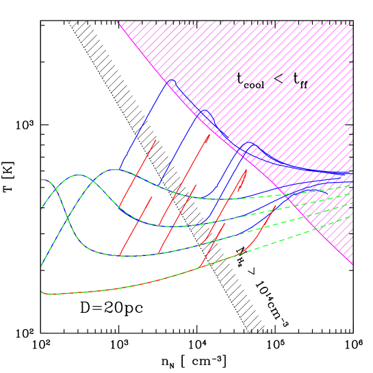
Figure 8: Evolutionary tracks on the central density v.s. temperature plane of the collapsing core are shown. Horizontal axis denotes the density of the core, whereas the vertical axis denotes the temperature. Dashed lines are the results of runs without radiative feedback, staring from four different initial conditions. Solid lines denote the case the results with radiative feedback for various ignition densities $n_{\rm on}$ and $D=20$pc, which in turn collapse successfully or fail to collapse. In the upper right shaded region, the condition $t_{\rm ff}>t_{\rm cool}$ is satisfied, whereas the upper right region bounded by thin dotted line shows the condition where the H$2$ column density of the core is larger than $10^{14}{\rm cm^{-2}}$, assuming equation (11).

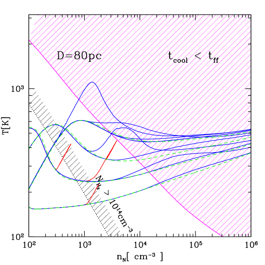
Figure 9: Same as Fig. 8, except that $D=80$pc.

Now the cooling conditions are shown in Figures 8 and 9 for two cases on density-temperature plane. Figure 8 corresponds to the case in which a $120M_{\odot}$ POPIII star is located 20 pc distant from the center of the collapsing core, whereas it is 80 pc in Figure 9. The horizontal axes denote the density at the center of the collapsing core, vertical axes are the temperature. The upper right hatched regions satisfy the cooling condition. The cooling condition $t_{\rm cool}<t_{\rm ff}$ ( corresponds to the hatched region) is obtained by directly solving equation (13). Note that the whole cooling region and its boundary satisfy $N_{\rm H_{2}}>10^{14}{\rm cm^{2}}$, which is required to derive equation (11). Thus, equation (13) based on equation (11) correctly describes cooling condition.

The dashed curves starting from the left side denote the evolutionary tracks on central density-temperature plane, with no feedback effects for various initial temperatures. . The solid lines which depart from the no feedback curves represent the cases where the photodissociation feedback is taken into consideration. In fact, the departing points from the dashed curves correspond to the timing when the nearby POPIII star is ignited.

We have two distinct classes of runs. First one is the case the LW band photons are effectively shielded. Thus, the cloud core is hardly affected by the feedback effect. Most of the runs in Figure 9 correspond to this case.

On the other hand, we also have the runs in which the LW band photons are not shield enough at the onset of the radiative feedback, which is immediately followed by the adiabatic collapse ($n_{\rm N}\propto T^{3/2}$). After this adiabatic phase, we also have two distinct classes of runs, one of which bounces, and the other collapses. The fate of the cloud is obviously determined by the cooling condition which we derived in this section: if the central density and temperature of the collapsing cloud can reach the cooling region, the collapse continues, otherwise it bounces. In other words, in case the cloud can shrink by the inertia until the cloud satisfies the cooling condition, the cloud can keep collapsing. If not, the collapse is stopped by the enhanced thermal pressure during the adiabatic contraction.

This results basically hold for both of the figures 8 and 9, in which different flux is assumed. It is also worth noting that the cooling criteria is independent of the initial cloud density and temperature, since it is written by some combination of various reaction rates and physical constants. In fact, all the calculations starting from different initial conditions evolve following the cooling criteria.

5.5 Comparison with the condition $t_{\rm dis}>t_{\rm ff}$

Now we compare the present results with simple criteria suggested by Glover & Brand (2001), i.e. $t_{\rm dis}>t_{\rm ff}$. However, it is difficult to compare our results directly with theirs since they assume fixed uniform cloud density and H₂ fraction. Therefore, we re-derive the condition for given $n_{\rm on}$ and $D$ which is equivalent to $t_{\rm dis}<t_{\rm ff}$, utilizing the relations found in the previous section.

Critical condition $t_{\rm dis}=t_{\rm ff}$ is obtained from the assumption that H₂ is in equilibrium:

$$k_{\rm 2step}y_{\rm H_{2}}=n_{\rm N}y_{\rm e}k_{\rm H^{-}}$$ (15)

and the dissociation time equals to the free fall time:

$$k_{\rm 2step}^{-1}=\sqrt{\frac{3\pi}{32Gm_{\rm p}n_{\rm N}}}.$$ (16)

Multiplying the two equations (15) (16), and using equation (6), we obtain

$$y_{\rm H_{2}}=\frac{k_{\rm H^{-}}}{k_{\rm rec}}.$$ (17)

Combining equations (17),(9) and (10), critical distance that satisfy $t_{\rm dis}=t_{\rm ff}$ for a given core density $n_{\rm N}$ and temperature $T$ is described as

$$D_{\rm cr}=113{\rm pc}\left(\frac{L_{\rm LW}}{10^{24}{\rm erg/s}}\right)^{-\frac{1}{2}}\left(\frac{n_{\rm N}}{10^{3}{\rm cm^{-3}}}\right)^{-\frac{7}{16}}\left(\frac{T}{600{\rm K}}\right)^{-\frac{3}{4}}.$$ (18)

Here we use the usual relation between the luminosity of the star($L_{\rm LW}$) and unshielded flux ($F_{\rm LW0}$),

$$4\pi F_{\rm LW0}D_{\rm cr}^{2}=L_{\rm LW}$$ (19)

Figure 10 shows the loci on $n_{\rm on}-D$ plane along which $t_{\rm dis}=t_{\rm ff}$ is satisfied (i.e. $D=D_{\rm cr}$) at the ignition time of the source star. Two lines correspond to the core temperatures (in equation 18) equal to $300$K and $400$K. If we consider $T_{\rm ini}=100$K case, the core temperatures at the turn-on time of the source star roughly satisfy $300{\rm K}\lesssim T\lesssim 400$K (see Figure 2). Thus, the actual condition $t_{\rm dis}=t_{\rm ff}$ would be between the two lines. Numerical results with $T_{\rm ini}=100$K are also superimposed on the $n_{\rm on}-D$ plane as the Figure 6.

Comparing the condition $t_{\rm dis}=t_{\rm ff}$ with the numerical results, we find that 1) the simple condition $t_{\rm dis}=t_{\rm ff}$ is not so bad, 2) but it overestimates the critical distance by a factor of 2-3. For comparison, we also plotted the distances that are factor $C$ times smaller than $D_{\rm cr}$ with $T=400$K. Five lines correspond to $C=0.1,0.2,0.3,0.4,0.5$, respectively. We find $C=0.3-0.4$ fit the numerical results better than the original condition $D=D_{\rm cr}$ does.

The disagreements between the condition $t_{\rm dis}=t_{\rm ff}$ and the numerical results basically comes from the dynamical effects of the collapsing gas. As discussed in the previous subsections, H₂ fraction in the collapsing core recovers very rapidly following the equation (11) during the adiabatic compression phase. As a result, dynamically contracting clouds can keep collapsing even if condition $t_{\rm dis}<t_{\rm ff}$ is satisfied when the source star is turned-on.

Figure 11 also shows the comparison of numerical results for $T_{\rm ini}=350$K with the criteria $t_{\rm dis}=t_{\rm ff}$. Since the core temperature at the turn-on time is approximately $100-200$K for this case, we plot the loci $t_{\rm dis}=t_{\rm ff}$ for $T=100$K and $200$K. In this case, we also find qualitatively the same results as above, however, the disagreement is slightly smaller than the previous case. In fact, we also plotted the loci along which $D=CD_{\rm cr}(200{\rm K})$ are satisfied for various $C$. In this case, $C=0.5-0.6$ gives a better fit to the numerical results. The smaller difference is due to the fact that the core temperature is so low at the turn-on time, that the adiabatic collapse is not enough to drive abundant H₂ formation.

In conclusion, $t_{\rm dis}>t_{\rm ff}$(i.e. $D>D_{\rm cr}$) gives a rough estimates, but we cannot neglect the dynamical effects on the H₂ formation.

6 Discussion

Present calculations are based upon the assumption that the collapsing gas is self-gravitating. This assumption would be correct for the prestellar cores formed by some fragmentation process of the shocked gas in large halos with $T_{\rm vir}\gtrsim 10^{4}$K. It is also relevant for the the collapsing dense prestellar cores ($n_{\rm N}\gtrsim 10^{3}{\rm cm^{{}^{-}3}}$) at the center of the very first halos formed directly from CDM density fluctuations. However, it would not be correct for the earlier phase (i.e. low density phase) of such prestellar cores with $n_{\rm N}\lesssim 10^{3}{\rm cm^{-3}}$, since dark matter halos are dominat source of gravity at such early phase. Thus, we have to consider the effect of dark matter for such low density cores. Ahn & Shapiro (2006) have performed one dimensional radiation hydrodynamics simulations on this issue. They take into account the effects by photoionization as well as the LW radiation. They also consider the effects of the age of POPIII stars. As a result, they find that net effect of radiation by a nearby star is approximately even. i.e. negative feedbacks balance with the positive feedbacks. These results could also be checked by our code in future.

LW-band radiation is basically the sum of line emissions, which should be treated carefully. Unfortunately, it is almost impossible to solve line transfer problem directly in huge three dimensional simulations by present computational resources. Therefore, we have employed the self-shielding function introduced by Draine & Bertoldi (1996). However, their formula is basically derived by the calculation for static slab, which might be irrelevant to the present issue. It is obvious that the self-shielding function is inappropriate to represent the absorption of the radiation in case the motion of the fluid element is supersonic. Therefore, the absorption by the gas in the envelope of the collapsing cloud would be over estimated, since the infalling envelope is supersonic(Larson, 1969). However, if the gas motion is not supersonic, the function gives a good estimate for the absorption of LW photons. In fact, in our numerical simulations, most of the absorption takes place in the collapsing core which is subsonic. Thus, we guess that we evaluate the absorption of LW radiation properly.

The effects of ionizing photons are obviously quite important, although it is not included in the present paper. Photoheating effects followed by the photoionization can leads negative feedback effects such as the photoevaporation of the cloud (e.g. Yoshida et al. 2006), creation of shock front (M-type I-front) which blow out the whole cloud(Susa & Umemura, 2006), whereas it also has positive feedback effects such as enhanced H₂ formation(Ahn & Shapiro, 2006), or formation of “H₂ barrier” between the source and the collapsing cloud(Susa & Umemura, 2006). This is a quite complicated problem, however, we also have performed numerical simulations on this issue. The details will be discussed in the forthcoming paper.

7 Summary

We perform radiation hydrodynamics simulations on the radiative feedback of POPIII stars. We obtain the well-understood collapse criteria of the primordial prestellar core both analytically and numerically in the presence of Lyman-Werner band photons from nearby stars. The criteria dictate the importance of self-shielding effects coupled with hydrodynamics. Consequently, the LW radiation from a POPIII star cannot halt the collapse of the dense clump($n_{\rm N}\gtrsim 10^{3}-10^{4}{\rm cm^{-3}}$) even if they are in the same halo. We also evaluate the effects of diffuse LW radiation background, which also is not important for the collapse of dense cores with $n_{\rm N}\gtrsim 10^{3}{\rm cm^{-3}}$.

We thank the anonymous referee for very careful reading and comments. We also thank N. Yoshida and M.Umemura for discussions and careful reading of the manuscript. N. Shibazaki and K. Ohsuga are acknowledged for continuous encouragements. The analysis has been made with computational facilities at Center for Computational Science in University of Tsukuba and Rikkyo University. This work was supported in part by Ministry of Education, Culture, Sports, Science, and Technology (MEXT), Grants-in-Aid, Specially Promoted Research 16002003 and Young Scientists (B) 17740110.

Figure 1: Density distribution of the collapsing cloud without radiative feedback. Two groups of dots represents the runs with $T_{\rm ini}=100$K and $350$K, at the epoch when the central part go below the resolution limit.

Figure 2: Evolution of the central core on density-temperature plane for various initial conditions. In these runs, the radiative feedback effects are not included.

Figure 5: H₂ fraction at the center of the cloud is shown as functions of time. Results from four runs are shown, in which $n_{\rm on}=10^{3}{\rm cm^{-3}},~{}T_{\rm ini}=100{\rm K}$, and $D=40,60,80,100$pc, respectively. The horizontal axis denotes the time after the collapse of the cloud is started. The ignition time of the nearby source star is marked by the arrow. Two solid line represent the case in which the cloud fails to collapse ($D=40$pc) and delayed collapse($D=60$pc), whereas the successful collapse cases are shown by the two dotted lines($D=80,100$pc).

Figure 6: Summary of numerical runs are shown on $n_{\rm on}-D$ plane. Four panels correspond to the runs with $T_{\rm ini}=50$K , 100K, 200K and 350K, respectively. Open circles denote the runs in which the clouds collapse successfully, whereas vertices represents the failed collapse.

Figure 7: Evolutionary tracks of electron fraction $y_{\rm e}$ are plotted against number density of the collapsing cloud. Each curve corresponds to a certain initial condition $(n_{\rm N0},y_{\rm e0})$.

Figure 10: The conditions $t_{\rm dis}=t_{\rm ff}$($D=D_{\rm cr}$) are plotted by solid lines on $n_{\rm on}-D$ plane for $T=300,400$K. Symbols represent the numerical runs. Open circles denote the runs in which the clouds collapse successfully, whereas vertices represents the failed collapse. The dotted lines represents the loci along which $D=CD_{\rm cr}(400K)$ are satisfied. $C=0.1,0.2,0.3,0.4,0.5$ corresponds to each line.

Figure 11: Same as Figure10, except that $T_{\rm ini}=350$K and the assumed core temperatures are $100$K and $200$K. The dotted lines represents the loci along which $D=CD_{\rm cr}(100K)$ are satisfied. $C=0.3,0.4,0.5,0.6,0.7$ corresponds to each line.

References

- Abel, Bryan, Norman (2000) Abel, T., Bryan, G. L., & Norman, M. L. 2000, ApJ, 540, 39
- Ahn & Shapiro (2006) Ahn, K. & Shapiro, P.R. 2006, astro-ph/0607642
- Baraffe, Heger & Woosely (2001) Baraffe, I., Heger, A. & Woosely, S.E. 2001, ApJ, 550, 890
- Barnes & Hut (1986) Barnes, J. & Hut, P., 1986, Nature, 324, 446
- Bromm, Coppi & Larson (2002) Bromm, V., Coppi, P., & Larson, R. 2002, ApJ, 564, 23
- Bromm & Larson (2004) Bromm, V & Larson, R. 2004, ARA&A, 42, 79
- Ciardi, Ferrara & Abel (2000) Ciardi, B., Ferrara, A., & Abel, T. 2000, ApJ, 533, 594
- Draine & Bertoldi (1996) Draine, B. T., & Bertoldi, F. 1996, ApJ, 468, 269
- Dubinski (1996) Dubinski, J. 1996, NewA, 1, 133
- Fukushige, Makino & Kawai (2005) Fukushige, T., Makino, J. & Kawai, A. 2005, astro-ph/0504407
- Galli & Palla (1998) Galli D. & Palla F. 1998, A&A, 335, 403
- Glover & Brand (2001) Glover, S & Brand, P. 2001, MNRAS, 321, 385
- Grief & Bromm (2006) Grief, T. & Bromm, V. 2006, preprint, astro-ph/0604367
- Hiaman, Rees & Loeb (1997) Haiman, Z., Rees, M. & Loeb, A., 1997, ApJ, 476, 458
- Hieneman et al. (2005) Heinemann, T., Dobler, W., Nordlund, A., Brandenburg, A. 2006, å,448, 731
- Iliev et al. (2006) Iliev, I. T., et al. 2006, MNRAS371, 1057
- Jhonson & Bromm (2006) Jhonson, J.L. & Bromm, V. 2006, MNRAS, 366, 247
- Kang & Shapiro (1992) Kang, H., & Shapiro, P., ApJ, 386, 432
- Larson (1969) Larson, R. 1969, MNRAS, 145, 271
- Machacek, Bryan & Abel (2001) Machacek, M.E., Bryan, G. L. & Abel, T. 2001, ApJ, 548, 509
- Meisinger, Bryan, & Haiman (2006) Meisinger,A., Bryan, G., & Haiman, Z. 2006, ApJ, 648, 835
- Nagakura & Omukai (2005) Nagakura, T. & Omukai, K. 2005, MNRAS, 363, 1378
- Nakamoto, Umemura, & Susa (2001) Nakamoto, T., Umemura, M., & Susa, H. 2001, MNRAS, 321, 593
- Nakamura & Umemura (1999) Nakamura F. & Umemura M. 1999, ApJ, 515, 239
- Nakamura & Umemura (2001) Nakamura, F., & Umemura, M. 2001, ApJ, 548, 19
- Oh & Haiman (2002) Oh, P & Haiman, Z. 2002, ApJ, 569, 558
- Omukai & Nishi (1998) Omukai, K. & Nishi, R. 1998, ApJ, 508, 141
- Omukai & Nishi (1999) Omukai, K. & Nishi, R. 1999, ApJ, 518, 64
- O’shea, Abel, Whalen & Norman (2005) O’Shea, B. W., Abel, T., Whalen, D., Norman, M. L. 2005, ApJ, 628, 5L
- O’shea & Norman (2006) O’Shea, B. W. & Norman, M. L. 2006, ApJ, 648, 31
- Penston (1969) Penston, M. V. 1969, MNRAS, 144, 425
- Ricotti, Gnedin, & Shull (2001) Ricotti, M. Gnedin, N. Y., Shull, M. 2001, ApJ, 560, 580
- Shapiro & Kang (1987) Shapiro, P.R., & Kang, H., 1987, ApJ, 318, 32
- Spitzer (1978) Spitzer, L. Jr. 1978, in Physical Processes in the Interstellar Medium (John Wiley & Sons, Inc. 1978)
- Steinmetz & Müller (1993) Steinmetz, M. & Müller, E. 1993, A&A, 268, 391
- Susa (2006) Susa, H. 2006, PASJ, 455, 58
- Susa & Kitayama (2000) Susa, H. & Kitayama, T. 2000, MNRAS, 317, 175
- Susa et al. (1998) Susa, H., Uehara, H., Nishi, R., & Yamada, M. 1998, Prog. Theor. Phys., 100, 63
- Susa & Umemura (2004a) Susa, H. & Umemura, M. 2004, ApJ, 600, 1
- Susa & Umemura (2004b) Susa, H. & Umemura, M. 2004, ApJ, 610, 5L
- Susa & Umemura (2006) Susa, H. & Umemura, M. 2006, ApJ, 645, 93L
- Thacker et al. (2000) Thacker, J., Tittley, R., Pearce, R., Couchman, P. & Thomas, A. 2000, MNRAS319, 619
- Uehara & Inutsuka (2000) Uehara, H. & Inutsuka, S., 2000, ApJ, 531, L91
- Umemura (1993) Umemura, M. 1993, ApJ, 406, 361
- Yoshida et al. (2003) Yoshida, N., Abel, T., Hernquist, L. & Sugiyama, N., 2003, ApJ, 592, 645
- Yoshida et al. (2006) Yoshida, N., Oh, P., Kitayama, T., & Hernquist, L., 2006, preprint, astro-ph/0610819