Particle acceleration at shock waves moving at arbitrary speed:
the case of large scale magnetic field and anisotropic scattering

Abstract

A mathematical approach to investigate particle acceleration at shock waves moving at arbitrary speed in a medium with arbitrary scattering properties was first discussed in Vietri (2003); Blasi $\&$ Vietri (2005). We use this method and somewhat extend it in order to include the effect of a large scale magnetic field in the upstream plasma, with arbitrary orientation with respect to the direction of motion of the shock. We also use this approach to investigate the effects of anisotropic scattering on spectra and anisotropies of the distribution function of the accelerated particles.

1 Introduction

The theory of particle acceleration at shock fronts moving with arbitrary speeds (from newtonian to ultra-relativistic) can be formulated in a simple and exact form Vietri (2003); Freiling, Vietri $\&$ Yurko (2003), at least in the so-called test particle limit, which neglects the dynamical reaction of accelerated particles on the shock. In this framework, all the basic physical ingredients can be taken into account in an exact way, with special reference to the type of scattering that is responsible for the particles to return to the shock front from the upstream and downstream plasmas. The information about scattering is introduced in the problem through a function $w(\mu,\mu^{\prime})$ which expresses the probability per unit length that a particle moving in the direction $\mu^{\prime}$ is scattered to a new direction $\mu$. It is worth stressing that $w$ can have a different functional form in the upstream and downstream plasmas, in particular in the case of relativistic shocks.

The repeated scatterings of the particles lead eventually to return to the shock front, as described in terms of the conditional probability $P_{u}(\mu_{0},\mu)$ ($P_{d}(\mu_{0},\mu)$) that a particle entering the upstream (downstream) plasma in the direction $\mu_{0}$, returns to the shock and crosses it in the direction of the downstream (upstream) plasma in the direction $\mu$. The mathematical method adopted to calculate the two very important functions $P_{u}$ and $P_{d}$ based upon the knowledge of the elementary scattering function $w$ was described in detail in Blasi $\&$ Vietri (2005), and is based on solving two non-linear integral-differential equations in the two independent coordinates $\mu_{0}$ and $\mu$.

Vietri (2003) showed on very general grounds that the spectrum of accelerated particles is a power law for all momenta exceeding the injection momentum. The slope of such power law and the anisotropy pattern of the accelerated particles near the shock front are fully determined by the conditional probabilities $P_{d}$ and $P_{u}$ and by the equation of state of the downstream plasma. Particle acceleration at shock fronts has been previously investigated through different methods, both semi-analytical (see for example Kirk $\&$ Schneider (1987); Gallant $\&$ Achterberg (1999); Kirk et al. (2000); Achterberg et al. (2001)) and numerical, by using Monte Carlo simulations (e.g. Bednard $\&$ Ostrowski (1998); Lemoine $\&$ Pelletier (2003); Niemiec $\&$ Ostrowski (2004); Lemoine $\&$ Revenu (2005)). The theory of particle acceleration developed by Vietri (2003) and Blasi $\&$ Vietri (2005) has been checked versus several of these calculations existing in the literature, both in the case of non relativistic shocks and for relativistic shocks, and assuming small as well as large pitch angle isotropic scattering (see Blasi $\&$ Vietri (2005) for an extensive discussion of these results).

In this paper we extend the application of this new theoretical framework to two new interesting situations: 1) presence of a coherent large scale magnetic field in the upstream fluid; 2) anisotropic scattering. In both cases we calculate the spectrum of accelerated particles and the distribution in pitch angle (upstream and downstream) for shock fronts moving with arbitrary velocity. The results of point 1) are compared with those obtained in Achterberg et al. (2001), carried out for a parallel ultra-relativistic shock.

The paper has been inspired by the need to address several points of phenomenological relevance. As far as relativistic shocks are concerned, it was understood that the return of the particles to the shock surface from the upstream region can be warranted even in the absence of scattering, provided the background magnetic field is at an angle with the shock normal (e.g. Achterberg et al. (2001)). This is due to the fact that the shock and the accelerated particles remain spatially close and regular deflection takes place before particles can experience the complex, possibly turbulent structure of the upstream magnetic field. This implies that the calculation of the spectrum of the accelerated particles cannot be calculated using a formalism based on the assumption of pitch angle diffusion, as in the vast majority of the existing literature.

In the downstream region, the motion of the shock is always quasi-newtonian, even when the shock moves at ultra-relativistic speeds. This implies that the propagation of the particles is generally well described by (small or large) pitch angle scattering. However, the turbulent structure of the magnetic field, responsible for the scattering, is likely to have an anisotropic structure and be therefore responsible for anisotropic scattering. In fact, even in the case of isotropic turbulence, the scattering can determine an anisotropic pattern of particle scattering. It follows that a determination of the spectrum able to take into account these potentially important situations is very important.

The outline of the paper is the following: in §2 we briefly summarize the theoretical framework introduced in Vietri (2003) and Blasi $\&$ Vietri (2005). In §3 we consider in detail the case of a large scale magnetic field in the upstream frame and no scattering of the particles. The scattering is assumed to be isotropic in the downstream plasma. In §4 we introduce the possibility of anisotropic scattering in both upstream and downstream plasmas. We summarize in §5.

2 An exact solution for the accelerated particles in arbitrary conditions: a summary

In this section we summarize the main characteristics of the theory of particle acceleration developed by Vietri (2003) and Blasi $\&$ Vietri (2005). The reader is referred to this previous work for further details. The power of this novel approach is in its generality: it provides an exact solution for the spectrum of the accelerated particles and at the same time the distribution in pitch angle that the particles acquire due to scattering in the upstream and downstream fluids. This mathematical approach is applicable without restrictions on the velocity of the fluid speeds (from newtonian to ultra-relativistic) and irrespective of the scattering properties of the background plasmas (small as well as large angle scattering, isotropic or anisotropic scattering). The only condition which is necessary for the theory to work is common to most if not all other semi-analytical approaches existing in the literature, namely that the acceleration must take place in the test particles regime: no dynamical reaction is currently introduced in the calculations. As a consequence, the shock is assumed to conserve its strength during the acceleration time, and the acceleration is assumed to have reached a stationary regime.

The directions of motion of the particles in the downstream and upstream frames are identified through the cosine of their pitch angles, all evaluated in the comoving frames of the fluids that they refer to. The direction of motion of the shock, identified as the $z$ axis, is assumed to be oriented from upstream to downstream, following the direction of motion of the fluid in the shock frame ($\mu=1$ corresponds to particles moving toward the downstream section).

The transport equation for the particle distribution function $g$, as obtained in Vietri (2003) in a relativistically covariant derivation reads

$$\gamma(u+\mu){\partial g\over\partial z}=\int\!\!\!\int\left[{-W(\mu^{\prime},\mu,\phi^{\prime},\phi)g(\mu,\phi)+W(\mu,\mu^{\prime},\phi,\phi^{\prime})g(\mu^{\prime},\phi^{\prime})}\right]d\mu^{\prime}d\phi^{\prime}+\omega{\partial g\over\partial\tilde{\phi}},$$ (1)

in which both scattering and regular deflection in a large scale magnetic field are taken into account.

Here all quantities are written in the fluid frame, with the exception of the spatial coordinate $z$, the distance from the shock along the shock normal, which is measured in the shock frame. $u$ and $\gamma$ are, respectively, the velocity and the Lorentz factor of the fluid with respect to the shock. $\theta$ and $\phi$ are the polar coordinates of particles in momentum space, measured with respect to the shock normal, while $\tilde{\phi}$ is the longitudinal angle around the magnetic field direction. As usual $\mu=\cos\theta$ and $\omega=eB/E$ is the particle Larmor frequency. $W(\mu,\mu^{\prime},\phi,\phi^{\prime})$ is the scattering probability per unit length, namely the probability that a particle moving in the direction ($\mu^{\prime},\phi^{\prime}$) is scattered to a direction ($\mu,\phi$) after travelling a unit length.

An important simplification of eq. (1) occurs when an axial symmetry is assumed. In this case the scattering probability depends only on $\Delta\equiv\phi-\phi^{\prime}$ and the large scale magnetic field can be either zero or different from zero but parallel to the shock normal. In both cases it is straightforward to integrate eq. (1) over $\phi$: the two-dimensional integral on the right-hand side simplifies to an integral in one dimension, while the term $\omega(\partial g/\partial\tilde{\phi})$ disappears.

These simplifications lead to

$$\gamma(u+\mu){\partial g\over\partial z}=\int\left[{-w(\mu^{\prime},\mu)g(\mu)+w(\mu,\mu^{\prime})g(\mu^{\prime})}\right]d\mu^{\prime},$$ (2)

where

$$w(\mu,\mu^{\prime}) \equiv \int W(\mu,\mu^{\prime},\Delta)\,d\Delta\qquad{\rm and}$$

$$g(\mu) \equiv {1\over 2\pi}\int g(\mu,\phi)\,d\phi\,.$$

The physical ingredients are all contained in the two conditional probabilities $P_{u}(\mu_{\circ},\mu)$ and $P_{d}(\mu_{\circ},\mu)$: these two functions provide respectively the probability that a particle entering the upstream (downstream) plasma along a direction $\mu_{0}$ exits it along a direction $\mu$. In the absence of large scale coherent magnetic fields, the two functions $P_{u}(\mu_{\circ},\mu)$ and $P_{d}(\mu_{\circ},\mu)$ were defined through a set of two integral-differential non linear equations by Blasi $\&$ Vietri (2005). We report these equations here for completeness:

$$P_{u}(\mu_{\circ},\mu)\left(\frac{d(\mu_{\circ})}{u+\mu_{\circ}}-\frac{d(\mu)}{u+\mu}\right)=\frac{w(\mu,\mu_{\circ})}{u+\mu_{\circ}}-\int_{-u}^{1}d\!\mu^{\prime}\frac{w(\mu,\mu^{\prime})P_{u}(\mu_{\circ},\mu^{\prime})}{u+\mu^{\prime}}+$$

$$\int_{-1}^{-u}d\!\mu^{\prime}\frac{w(\mu^{\prime},\mu_{\circ})P_{u}(\mu^{\prime},\mu)}{u+\mu_{\circ}}-\int_{-1}^{-u}d\!\mu^{\prime}P_{u}(\mu^{\prime},\mu)\int_{-u}^{1}d\!\mu^{\prime\prime}\frac{w(\mu^{\prime},\mu^{\prime\prime})P_{u}(\mu_{\circ},\mu^{\prime\prime})}{u+\mu^{\prime\prime}},$$ (3)

$$P_{d}(\mu_{\circ},\mu)\left(\frac{d(\mu_{\circ})}{u+\mu_{\circ}}-\frac{d(\mu)}{u+\mu}\right)=\frac{w(\mu,\mu_{\circ})}{u+\mu_{\circ}}+\int_{-u}^{1}d\!\mu^{\prime}\frac{P_{d}(\mu^{\prime},\mu)w(\mu^{\prime},\mu_{\circ})}{u+\mu_{\circ}}-$$

$$\int_{-1}^{-u}d\!\mu^{\prime}\frac{P_{d}(\mu_{\circ},\mu^{\prime})w(\mu,\mu^{\prime})}{u+\mu^{\prime}}-\int_{-u}^{1}d\!\mu^{\prime}P_{d}(\mu^{\prime},\mu)\int_{-1}^{-u}d\!\mu^{\prime\prime}\frac{w(\mu^{\prime},\mu^{\prime\prime})P_{d}(\mu_{\circ},\mu^{\prime\prime})}{u+\mu^{\prime\prime}}.$$ (4)

In the equations above we used:

$$d(\mu)\equiv\int_{-1}^{+1}w(\mu^{\prime},\mu)d\!\mu^{\prime}\;,$$ (5)

which is unity by definition.

It is worth stressing that Eq. (2) provides automatically the correct normalization for the return probability from upstream: $\int_{-u}^{1}d\mu^{\prime}P_{u}(\mu_{\circ},\mu^{\prime})=1$, independent of the entrance angle $\mu_{\circ}$. In §3 we will generalize the method to include the possibility of deflection by large scale magnetic fields, which is one of the achievements of this work. In that case we will show that the return probability from upstream is no longer bound to be unity, due to the escape of particles from the upstream region.

The procedure for the calculation of the slope of the spectrum of accelerated particles, as found by Vietri (2003) and Blasi $\&$ Vietri (2005), is as follows: for a given Lorentz factor of the shock ($\gamma_{s}$), the velocity of the upstream fluid $u=\beta_{s}$ is calculated. The velocity $u_{d}$ of the downstream fluid is found from the usual jump conditions at the shock and through the adoption of an equation of state for the downstream fluid.

Once the two functions $P_{u}$ and $P_{d}$ have been calculated, the slope of the spectrum, as discussed in Vietri (2003), is given by the solution of the integral equation:

$$(u_{d}+\mu)g(\mu)=\int_{-u_{d}}^{1}d\xi Q^{T}(\xi,\mu)(u_{d}+\xi)g(\xi),$$ (6)

where

$$Q^{T}(\xi,\mu)=\int_{-1}^{-u_{d}}d\nu P_{u}(\nu,\mu)P_{d}(\xi,\nu)\left(\frac{1-u_{rel}\mu}{1-u_{rel}\nu}\right)^{3-s}.$$ (7)

Here $u_{rel}=\frac{u-u_{d}}{1-uu_{d}}$ is the relative velocity between the upstream and downstream fluids and $g(\mu)$ is the angular part of the distribution function of the accelerated particles, which contains all the information about the anisotropy. Note that in Eq. (7) all variables and functions are evaluated in the downstream frame, while the $P_{u}$ calculated through Eq. (3) is in the frame comoving with the (upstream) fluid. The $P_{u}$ that need to be used in Eq. (7) is therefore

$$P_{u}(\nu,\mu)=P_{u}(\tilde{\nu},\tilde{\mu})\frac{d\tilde{\mu}}{d\mu}=P_{u}(\tilde{\nu},\tilde{\mu})\left[\frac{1-u_{rel}^{2}}{(1-u_{rel}\mu)^{2}}\right].$$

The solution for the slope $s$ of the spectrum is found by solving Eq. (6). In general, this equation has no solution but for one value of $s$. Finding this value provides not only the slope of the spectrum but also the angular distribution function $g(\mu)$.

2.1 The special case of isotropic scattering

No assumption has been introduced so far about the scattering processes that determine the motion of the particles in the upstream and downstream plasmas, with the exception of the axial symmetry of the function $W(\mu,\mu^{\prime},\phi,\phi^{\prime})$.

A special case of this symmetric situation is that of isotropic scattering, that takes place when the scattering probability $W$ only depends upon the deflection angle $\Theta$, related to the initial and final directions through

$$\cos\Theta\equiv\mu\mu^{\prime}+\sqrt{1-\mu^{2}}\sqrt{1-\mu^{\prime 2}}\cos(\phi-\phi^{\prime}).$$ (8)

Among the many functional forms that correspond physically to isotropic scattering, the simplest one is

$$W(\mu,\mu^{\prime},\phi,\phi^{\prime})=W(\cos\Theta)={1\over\sigma}e^{-{1-\cos\Theta\over\sigma}}\,,$$ (9)

where $\sigma$ is the mean scattering angle. Integration of eq. (9) over $\phi-\phi^{\prime}$ leads to

$$w(\mu,\mu^{\prime})={1\over\sigma}e^{-{1-\mu\mu^{\prime}\over\sigma}}I_{0}\left({\sqrt{1-\mu^{2}}\sqrt{1-\mu^{\prime 2}}\over\sigma}\right)\,,$$ (10)

with $I_{0}(x)$ the Bessel function of order 0. Eq. (9), first introduced in Blasi $\&$ Vietri (2005), naturally satisfies the requirement of being symmetric under rotations around the normal to the shock surface. In the limit $\sigma\ll 1$ this function becomes a Dirac Delta function, strongly peaked around the forward direction, corresponding to isotropic Small Pitch Angle Scattering (SPAS). For the opposite limit, that is $\sigma\gg 1$, $w$ becomes flat and corresponds to the case of isotropic Large Angle Scattering (LAS). In §4.1 we will modify this functional form to introduce the possibility of anisotropic scattering.

3 Deflection by a regular magnetic field in the upstream region

It is well known that particle acceleration at a shock front with parallel magnetic field without scattering centers does not work. This magnetic scattering may be self-generated by the same particles, but the process of generation depends on the conditions in specific astrophysical environments. The case in which a regular magnetic field not parallel to the shock normal is present in the upstream fluid is quite interesting in that it allows for the return of the particles to the shock front even in the absence of scattering. In this section we investigate in detail the process of acceleration at shocks with arbitrary velocity when only a regular large scale magnetic field is present upstream (no scattering). We assume that enough turbulence is instead present in the downstream plasma to guarantee magnetic scattering of the particles.

There are two main differences introduced by this situation when compared with the standard case considered in the previous section:

• (a) Particle motion in the upstream region is deterministic: the stochasticity introduced by the interaction with scattering centers is assumed to be absent. This requires a new determination of the return probability $P_{u}$ introduced above.

• (b) The presence of regular magnetic field with arbitrary orientation breaks the axial symmetry around the shock normal. This, in principle, would force us to treat the problem in the four angular variables $\mu_{\circ},\phi_{\circ},\mu$ and $\phi$.

In the following we will show how addressing point (a) in fact solves point (b) as well.

3.1 Upstream return probability

Let us Consider a particle entering upstream in the direction identified by the two angles $\mu_{\circ}$ and $\phi_{\circ}$, and returning to the shock along the direction identified by $\mu$ and $\phi$. Since the motion of the particle is deterministic, the return direction is completely defined by the incoming coordinates, and we can write in full generality:

$$P_{u}(\mu_{\circ},\phi_{\circ};\mu,\phi)={(2\pi)}^{-1}\delta\left(\mu-\mu_{1}(\mu_{\circ},\phi_{\circ})\right)\,\delta\left(\phi-\phi_{1}(\mu_{\circ},\phi_{\circ})\right)\,,$$ (11)

where $\mu_{1}$ and $\phi_{1}$ are obtained from the solution of the equation of motion, as discussed below. One can see that $P_{u}$ is effectively a function of only two variables.

In order to apply the same mathematical procedure introduced in §2, we need to write $P_{u}$ as a function of azimuthal angles only. Therefore we use the properties of the delta function in $\delta(\mu-\mu_{1}(\mu_{\circ},\phi_{\circ}))$, to write:

$$P_{u}(\mu_{\circ},\phi_{\circ};\mu,\phi) = {1\over 2\pi}\left|{\partial\phi_{\circ}(\mu_{\circ},\mu)}\over\partial\mu\right|\,\delta\left(\phi_{\circ}-\bar{\phi_{\circ}}\right)\,\delta\left(\phi-\phi_{1}\right)$$ (12)

$$\equiv P_{u}(\mu_{\circ},\mu)\,\delta\left(\phi_{\circ}-\bar{\phi_{\circ}}\right)\,\delta\left(\phi-\phi_{1}\right)\,.$$

We now show that $P_{u}(\mu_{\circ},\mu)$, as defined by Eq. (12), is exactly the function to be used in eq. (7). This is easily shown by writing the fluxes of particles ingoing and outgoing the upstream plasma:

$$J_{+}(\mu,\phi)=\int_{-1}^{-u}d\mu^{\prime}\int_{0}^{2\pi}d\phi^{\prime}\,P_{u}(\mu^{\prime},\phi^{\prime},\mu,\phi)J_{-}(\mu^{\prime},\phi^{\prime})\,,$$ (13)

which, when integrated over $\phi$, yields

$$J_{+}(\mu)\equiv\int d\phi J_{+}(\mu,\phi)=\int_{-1}^{-u}d\mu^{\prime}\,P_{u}(\mu^{\prime},\mu)J_{-}(\mu^{\prime})\,,$$ (14)

where we assumed that $J_{-}$ is independent of $\phi$. This is exactly the same relationship as was used in Vietri (2003), and proves our point that the system may, in the average, still be treated as if it were symmetric about the shock normal.

The key assumption here is that the flux crossing back into the upstream region from the downstream one, $J_{-}$, be independent of the azimuthal angle $\phi$. This is of course true in the Newtonian regime, because there the residence time for all particles diverges, and there is time for deflections to effectively erase anisotropies in the $\phi$ direction. But this must be true a fortiori in the relativistic regime, when one considers that the properties of scattering are of course still the same as in the Newtonian regime, while the surface to be recrossed, i.e., the shock, is running away from the particles at a speed that becomes, asymptotically, a fair fraction of the particles’ speed. So, while not exactly true, the independence of $J_{-}$ from $\phi$ is at least a good approximation.

In order to write $P_{u}(\mu_{\circ},\mu)$ in a more explicit way, we need to solve the equation of motion of the particles, namely find the direction at which the particles re-cross the shock front as a function of the incoming direction. Particles move following a helicoidal trajectory around the magnetic field direction, indicated here as $\tilde{z}$. The problem is simplest if expressed in the frame $\tilde{O}$ comoving with the upstream fluid but with the polar axis coincident with $\tilde{z}$. We mark with a tilde all quantities expressed in this frame. The equations of motion in the frame $\tilde{O}$ are:

$$\tilde{\mu}(t) = \tilde{\mu}_{\circ}\,,$$ (15)

$$\tilde{\phi}(t) = \tilde{\phi}_{\circ}+\omega t\,,$$ (16)

where $t$ is time and $\omega$ is the Larmor frequency. The particles re-cross the shock when $z_{\rm particle}(t)=z_{\rm shock}(t)$. This condition expressed in the frame $\tilde{O}$ reads

$$\sin(\omega\,t+\tilde{\phi}_{\circ})-\sin\tilde{\phi}_{\circ}={\tilde{\mu}_{\circ}\,\cos\alpha+\beta_{s}\over\sin\alpha\>\sin\tilde{\theta}_{\circ}}\>\omega t\,,$$ (17)

where $\alpha$ is the angle between the shock normal $z$ and the magnetic field direction $\tilde{z}$. The solution of Eq. (17) gives the upstream residence time $t^{*}$ of the particles, to be evaluated numerically.

The angles that identify the re-crossing direction, as functions of the residence time, are

$$\tilde{\mu}_{1} = \tilde{\mu}_{\circ}\,,\qquad{\rm and}$$ (18)

$$\tilde{\phi}_{1} = \tilde{\phi}_{\circ}+\omega t^{*}(\tilde{\mu}_{\circ},\tilde{\phi}_{\circ})\,.$$ (19)

A rotation by the angle $\alpha$ provides us with the re-crossing coordinates $\mu_{1}$ and $\phi_{1}$ in the fluid frame. At this point the Jacobian in Eq. (12) can be calculated, although some care is needed because this Jacobian is not a single valued function: for each pair ($\mu_{\circ},\mu$) the Jacobian has two values. This degeneracy arises because of the substitution of $\phi_{\circ}$ with $\mu$, since each $\mu$ corresponds in general to two possible values of $\phi_{\circ}$. This is clear from fig. 1, where we show some examples of solutions: the directions of entrance and escape from the upstream fluid are plotted for different values of the shock speed and for different orientations of the large scale magnetic field.

Figure 1: Location of the particles entering the upstream region (dashed lines) and returning to the downstream region (solid lines) after being deflected by the magnetic field upstream. The directions are plotted in the plane $\Gamma_{s}\beta_{p,x}$ - $\Gamma_{s}\beta_{p,y}$. $\beta_{p,x}$ and $\beta_{p,y}$ are the components of the particle velocity along the $x$ and the $y$ axis respectively. The origin corresponds to particles entering along the shock normal. Circles correspond to particles having constant $\mu_{\circ}$. The upper panels refer to $\Gamma_{s}\beta_{s}=0.04$. The lower panel refer to $\Gamma_{s}\beta_{s}=1.0$. In both cases we show the effects of three different orientations of the magnetic field (from left to right $\cos\alpha=0.0,0.4,0.8$). The presence of an empty region when $\cos\alpha>\beta_{s}$ is due to particle leakage from upstream [Compare with fig.1 in Achterberg et al. (2001).]

Eq. (17) admits a solution $t^{*}>0$ only if the two following conditions are fulfilled:

• the initial velocity of a particle along the shock normal must be larger than the shock speed (otherwise the particle is prevented from crossing the shock to start with). This implies:

  $$\mu_{\circ}<-\beta_{s}\,.$$ (20)

• The particle velocity along the shock normal has to be less than the shock speed, namely

  $$\tilde{\mu}_{\circ}\,\cos\alpha>-\beta_{s}\,.$$ (21)

Particles not satisfying this last condition escape the shock region towards upstream infinity, a situation which is not realized in the case of scattering considered in §2. This escape process occurs only for $\cos\alpha>-\beta_{s}$, and results in the loss of particles having the entrance pitch angles cosine exceeding $\mu_{\rm min}(\mu_{\circ},\phi_{\circ})$. In fact for $\cos\alpha<-\beta_{s}$, $\mu_{\rm min}={\rm const}=-1$ and all particles eventually re-cross the shock.

When the particles are allowed to escape upstream, the acceleration is clearly expected to become less efficient and give rise to softer spectra of the accelerated particles (see §3.2).

Putting together all of the above, we can finally write the upstream conditional probability as

$$P_{u}(\mu_{\circ},\mu)={1\over 2\pi}\sum_{i=1,2}\left|{\partial\phi_{\circ}}\over\partial\mu\right|_{i}\theta(-\mu_{\circ}-\beta_{s})\,\theta(\mu_{\circ}-\mu_{\rm min}(\mu_{\circ},\mu))\,,$$ (22)

where the sum is extended over the two branches of the Jacobian.

For $\cos\alpha<-\beta_{s}$ the particles always return to the shock front and this forces the return probability to be unity when integrated over all outgoing directions:

$$\int_{-u}^{1}d\mu\,P_{u}(\mu_{\circ},\mu)=1\,.$$ (23)

This integral condition is trivially satisfied by Eq. (22) and is used as a check for $P_{u}$ after its numerical computation.

Figs. 2, 3 and 4 show some examples of our calculations of $P_{u}(\mu_{\circ},\mu)$ as a function of $\mu$ for different values of $\mu_{\circ}$, for a Newtonian, a trans-relativistic and a relativistic shock respectively. For each case we show the results for different inclinations of the magnetic field with respect to the shock normal. It is worth noticing that $P_{u}$ does not change significantly when the inclination of the magnetic field varies in the range $0<\cos\alpha<\beta_{s}$, at a given shock speed. Therefore we do not expect a significant variation of the spectral slope in this range. In §3.2 we show that this is in fact the case.

Figure 2: Conditional probability $P_{u}(\mu_{\circ},\mu)$ as a function of the outgoing direction $\mu$, for a fixed value of the shock speed ($\Gamma_{s}\beta_{s}=0.04$) with three different inclinations of the magnetic field ($\cos\alpha=0.0,0.4,0.9$). For each plot the different lines correspond to different values of the ingoing direction $\mu_{\circ}$.

Figure 3: Like fig.2 but for a trans-relativistic shock ($\Gamma_{s}\beta_{s}=1.0;\beta_{s}=0.707$).

Figure 4: Like fig.2 but for a relativistic shock ($\Gamma_{s}\beta_{s}=5.0;\beta_{s}=0.98$). The three plots are very similar to each other because the condition $\cos\alpha>\beta_{s}$ is never reached.

3.2 Spectrum and Anisotropy of the accelerated particles for a large scale magnetic field upstream

In this section we use Eq. (6) and Eq. (7) to calculate the spectrum and angular distribution of the accelerated particles at the shock front. The return probabilities are calculated assuming that in the downstream fluid there is isotropic scattering, so that $P_{d}$ can be calculated from Eq. (2) using Eq. (10) as a scattering function. We assume $\sigma=0.01$ for the SPAS regime and $\sigma=10$ for the LAS regime. In the upstream fluid we assume that particles can only be deflected by a large scale coherent magnetic field with arbitrary orientation with respect to the normal to the shock front. The return probability $P_{u}$ is therefore calculated as discussed in detail in §3.1.

The only information still lacking to proceed further is an equation of state for the medium, that would allow us to compute the velocity of the downstream fluid from the jump conditions at the shock front (see for instance Gallant (2002)). We assume that the gas upstream has zero pressure. Moreover, in the following we assume everywhere that the magnetic field has no dynamical role, so that the standard jump conditions for an unmagnetized shock can be adopted (the role of the magnetic field becomes important when the magnetic energy density becomes comparable with the thermal energy density Kirk $\&$ Duffy (1999)).

Following much of the previous literature, we adopt the Synge equation of state for the downstream gas Synge (1957), assuming that only protons contribute. Although used widely, this assumption may not be well justified in a general case. We will illustrate our conclusions on the role of the equation of state for the spectrum and anisotropy of the accelerated particles in a separate paper.

Within this set of assumptions it is worth reminding that the compression ratio $u_{\rm up}/u_{\rm down}$ tends asymptotically to $4$ for a non relativistic shock (even for shock speeds that are known to give lower compression factors) and to $3$ for ultra-relativistic shocks.

The simplest case to consider is that of a shock in which the large scale coherent magnetic field in the upstream region is parallel to the shock front ($\cos\alpha=0$). This is known as a perpendicular shock. The angular distribution and the slope of the spectrum of the accelerated particles are plotted in Fig. 5 (the LAS (SPAS) case is shown in the left (right) panel) and Fig. 6 respectively, for various shock velocities ranging from newtonian to relativistic.

The angular distribution of the particles in the downstream frame is seen to be rather anisotropic for the SPAS case, even in the newtonian regime. Large angle scattering (LAS) is evidently more efficient in isotropizing the accelerated particles. The anisotropies do not seem to affect the spectrum of the accelerated particles in the case of non relativistic shocks: the slope of the spectrum for both SPAS and LAS is $4.000\pm 0.001$. The effect becomes more prominent for faster shocks and in particular for relativistic shocks. In the SPAS case, for $\Gamma_{s}\beta_{s}=10$, we found $s=4.272\pm 0.001$, compatible with $s=4.28\pm 0.01$, obtained by Achterberg et al. (2001) for $\Gamma_{s}=10$, with a Monte-Carlo simulation.

In Fig. 6, the dotted and dashed lines refer to the SPAS and LAS cases respectively. At first sight it may appear rather surprising that in the limit of relativistic shocks the spectrum of accelerated particles is softer in the LAS regime than it is in the SPAS regime, since LAS is envisioned as more efficient in redirecting the particles to the shock front. This intuitive vision turns out to be incorrect, as also shown in Table 1, where we list the slope, the average energy gain and the return probability from downstream (as defined in Eqs. (26) and (29)) for a relativistic shock with $\Gamma_{s}\beta_{s}=5.0$.

Table 1: Exact spectral slope, mean amplification and downstream return probability (as defined in eq. (26) and (29) respectively) for $\Gamma_{s}\beta_{s}=5.0$.

	slope	$\langle G\rangle$	$\langle P_{\rm ret}^{\rm(down)}\rangle$
SPAS	$4.218\pm 0.001$	2.0387	0.4165
LAS	$4.445\pm 0.001$	2.0753	0.3430

One can see that while the average energy gain is similar in the two cases, the return probability in the case of LAS is 20% lower than for the SPAS case. Qualitatively this can be understood as follows: when the shock velocity increases, particles are caught up by the shock front when they have travelled only a small fraction (of order $1/\Gamma_{s}$) of their gyration. Once downstream, LAS is likely to swing them far from the shock front in a few interactions, while SPAS deflects their trajectories rather slowly yet remaining in the vicinity of the shock surface. This is responsible for the 20% difference in the average return probabilities in the two cases. This is also shown in Fig. 7, where we plot the particles flux, $J(\mu)\equiv|\mu+u_{d}|g(\mu)$ in terms of downstream coordinates: the total flux of particles entering the downstream section ($-u_{d}<\mu<1$) is normalized to unity. It is clear from Fig. 7 that the flux of particles returning to the shock is slightly larger for the case of SPAS (dashed line in the range $-1<\mu<-u_{d}$).

Figure 5: Particle distribution function at the shock front when a large scale coherent magnetic field is present in the upstream region, with a direction parallel to the shock plane. In the downstream region particles are scattered in the LAS (left plot) or in the SPAS regime (right plot) (here the maximum of is arbitrarily set equal to 1). Several values of shock speeds are shown. The particle distribution functions always show a jump at $\mu=-\beta_{s}$. Large angle scattering makes distribution functions flatter compared with the small angle scattering case for $-1<\mu<-u_{d}$.

Figure 6: Spectral index vs. shock speed for the same configuration as in fig.5.

Figure 7: Particle flux $J(\mu)\equiv|\mu+u_{d}|g(\mu)$ across the shock front, as it appears in the downstream frame, when the upstream magnetic field is parallel to the shock ($\cos\alpha=0$) and the downstream fluid is in the LAS regime (solid line) or SPAS regime (dashed line). The shock speed is $\Gamma_{s}\beta_{s}=5.0$. The flux entering downstream (i.e. for $-u_{d}<\mu<1$) is normalised to $1$. In this way we see that downstream return probability, i.e. the integrated flux for $-1<\mu<-u_{d}$, is larger when the downstream region is in the SPAS regime.

A more interesting question concerns the effect of the orientation of the large scale magnetic field with respect to the normal to the shock. We have already emphasized that for any orientation different from that of a perpendicular shock, and in the absence of scattering processes upstream, particles are lost from the upstream region, because the shock cannot catch up with their motion. This happens when $\cos\alpha>-\beta_{s}$, so that the phenomenon is increasingly more important for shocks approaching the parallel configuration. This reflects in increasingly softer spectra. In the limit $\cos\alpha\rightarrow 1$, all particles escape from the upstream region and no acceleration takes place.

The slope of the spectrum as obtained from our calculations is plotted in Fig. 8 (solid lines and symbols) as a function of $\cos\alpha$ for three different shock speeds ($\Gamma_{s}\beta_{s}=0.6,1.0,2.0$): when there is no particle escape, the slope $s$ is actually a constant, while it increases dramatically (and in fact diverges, showing the disappearance of the acceleration process) for values of $\cos\alpha$ larger than $-\beta_{s}$. In the small panel in Fig. 8 we also plot the return probability from upstream: for very inclined shocks the return probability is still very close to unity, as in the case of upstream scattering, but it drops rapidly for increasingly less inclined shocks.

The steepening of the spectrum due to leakage of the particles towards upstream infinity can also be understood in terms of a Bell-like Bell (1978) calculation, when carried out for the case of a large scale coherent magnetic field. The slope of the spectrum is related to the average return probability and to the average energy gain of the particles per cycle back and forth through the shock front through the expression:

$$s=3-{\log\langle P_{\rm ret}\rangle\over\log\langle G\rangle},$$ (24)

where $\langle G\rangle$ is the mean amplification in a single cycle (downstream $\rightarrow$ upstream $\rightarrow$ downstream), and $\langle P_{\rm ret}\rangle$ is the mean probability of returning to the shock. One should keep in mind that Bell’s method, as expressed through the equation above is flawed in that it does not take into proper consideration the correlation between the amplification factor and the return probability. Moreover, Eq. (24) hides the assumption of isotropy of the distribution function of the accelerated particles, since that formula was conceived in a discussion of non relativistic shocks (Peacock (1981) introduced this formalism for particle acceleration at relativistic shock fronts). All these limitations become of particular importance for relativistic shocks. A general expression for the slope was found in Vietri (2003), and reads:

$$\langle P_{\rm ret}\rangle\langle G^{s-3}\rangle=1.$$ (25)

In the following we use Eq. (24), since we only want to provide the reader with an argument of plausibility for the steepening of the spectra in those cases in which particle leakage can take place in the upstream region. In order to account for this leakage, which cannot take place in the standard scenario of diffusive particle acceleration at a shock front, we generalize Eq. (24) in order to include the probability of escape from the acceleration box from upstream. This is easily achieved by replacing $\langle P_{\rm ret}\rangle$ with $\langle P_{\rm ret}^{\rm(up)}\rangle\cdot\langle P_{\rm ret}^{\rm(down)}\rangle$. These mean values expressed in the downstream frame are:

$$\langle P_{\rm ret}^{\rm(down)}\rangle=\frac{\int_{-1}^{-u_{d}}d\mu_{\circ}\,\int_{-u_{d}}^{1}d\mu\,g(\mu)(u_{d}+\mu)P_{d}(\mu,\mu_{\circ})}{\int_{-u_{d}}^{1}d\mu\,g(\mu)(u_{d}+\mu)}$$ (26)

and

$$\langle P_{\rm ret}^{\rm(up)}\rangle=\frac{\int_{-u_{d}}^{1}d\mu\int_{-1}^{-u_{d}}d\mu_{\circ}\,g(\mu_{\circ})(u_{d}+\mu_{\circ})P_{u}(\mu_{\circ},\mu)}{\int_{-1}^{-u_{d}}d\mu_{\circ}\,g(\mu_{\circ})(u_{d}+\mu_{\circ})}\,.$$ (27)

In the last equation $P_{u}$ has also to be computed in terms of quantities evaluated in the downstream frame. Energy amplification for a particle entering the upstream region with direction $\mu_{\circ}$ (as measured downstream) and returning with direction $\mu$, is obtained combining two Lorentz transformations:

$$G(\mu_{\circ},\mu)=\gamma_{\rm rel}^{2}(1-u_{\rm rel}\mu_{\circ})\,\left(1+u_{\rm rel}\bar{\mu}\right)\,,$$ (28)

where $\bar{\mu}=(\mu+u_{\rm rel})/(1+u_{\rm rel}\mu)$ is the returning direction as seen in the upstream frame. Averaging the amplification we have:

$$\langle G\rangle=\frac{\int_{-1}^{-u}d\mu_{\circ}\,g(\mu_{\circ})(u+\mu_{\circ})\int_{-u}^{1}d\mu\,G(\mu_{\circ},\mu)P_{u}(\mu_{\circ},\mu)}{\int_{-1}^{-u}d\mu_{\circ}\,g(\mu_{\circ})(u+\mu_{\circ})\int_{-u}^{1}d\mu\,P_{u}(\mu_{\circ},\mu)}\,.$$ (29)

The spectral slope as computed through Eq. (24) is plotted in Fig. 8 (large box) with dashed lines; the corresponding upstream return probability $\langle P_{\rm ret}^{\rm(up)}\rangle$ is plotted in the small box (dashed lines). The agreement with our exact results is better than $1\%$, proving that the reason for the softening of the spectra of accelerated particles is in the increased probability that the particles leave the acceleration region when only a large scale coherent magnetic field is present upstream.

Figure 8: Large box: spectral slope as a function of $\cos\alpha$ for three different values of the shock speed. The dashed lines show the spectral slope computed with Bell’s method. Small box: the corresponding upstream return probabilities.

The results discussed above apply to situations in which the magnetic field in the upstream region can be considered as coherent on spatial scales exceeding the size of the acceleration box. If the coherence scale of the field is smaller than the size of the accelerator, then the direction of the particles suffer a random wandering motion and one can think of this structured field as the source of diffusion and as a physical mechanism that imposes a maximum energy to the accelerated particles (at least in the absence of radiative energy losses). Particles that escape from the shock region too fast (highest energy ones) have enough time to feel the effect of a coherent scale, while lower energy particles live in the accelerator for longer times and in principle may feel different orientations of the upstream magnetic field. This scenario is basically equivalent to having some degree of scattering upstream, and should be treated with the formalism already discussed in Vietri (2003); Blasi $\&$ Vietri (2005). As soon as a phenomenon equivalent to scattering is present, the probability of escape to upstream infinity vanishes, for all those particles that are confined in the accelerator for sufficiently long times. Moreover, one should keep in mind that even if a large scale coherent magnetic field is present to start with, the propagation of the accelerated (charged) particles in the upstream plasma is very likely to excite fluctuations in the magnetic field structure through streaming instability Bell (1978). These fluctuations act as scattering centers and enhance the probability of returning to the shock front.

4 Anisotropic scattering

In this section we consider again the standard case in which particle motion in both the upstream and downstream fluids is diffusive, due to the presence of scattering agents. However, we include the possibility that the scattering, though spatially constant, may be anisotropic. The physical motivation for this generalization is the following: in a background of Alfvèn waves with a power spectrum $P_{W}(k)$ (such that $P_{W}(k)dk$ is the energy density in the form of waves with wavenumber in the range $dk$ around $k$) the particles suffer angular diffusion with a diffusion coefficient

$$D_{\theta\theta}=\langle\frac{\Delta\theta\Delta\theta}{\Delta t}\rangle\approx\Omega\frac{k_{r}P_{W}(k_{r})}{B_{0}^{2}/8\pi},$$ (30)

where $k_{r}=\Omega/v\mu$ is the resonant wavenumber and $\Omega$ is the gyration frequency of particles with momentum $p$ in the background magnetic field $B_{0}$. One can clearly see from Eq. (30) that the diffusion is anisotropic in general, unless the power spectrum has a specific ad hoc form. One should keep in mind that Eq. (30) is obtained in the context of quasi-linear theory. A full non-linear treatment might show how the turbulence is distributed and which is the resulting particle angular distribution.

In the calculations that follow, we quantify the effects of anisotropic scattering on the spectrum and angular distribution of the accelerated particles. The calculation of specific patterns of anisotropy in the scattering agents is beyond the scopes of this paper, therefore we adopt a few simple but physically meaningful toy models of anisotropic scattering and we carry out the calculations within those models.

4.1 Modelling anisotropy

We parametrize the anisotropy in such a way to reproduce the following four patterns:

• case A: Particles are scattered per unit length more efficiently while they move away from the shock front than they are on their way to the shock front, both upstream and downstream.

• case B (opposite of case A): Particles are scattered per unit length more efficiently on their way to the shock front than they are while they move away from the shock front, both upstream and downstream.

• case C: In the downstream fluid, particles are scattered per unit length more efficiently while they move away from the shock front ($\mu\to 1$) than they are on their way to the shock front ($\mu\to-1$). In the upstream fluid the situation is reversed, and scattering is more efficient for the particles that are moving toward of the shock ($\mu\to 1$).

• case D (opposite of C): Scattering is more effective around $\mu\sim-1$ both upstream and downstream.

A pictorial representation of cases A-D is shown in Fig. 9.

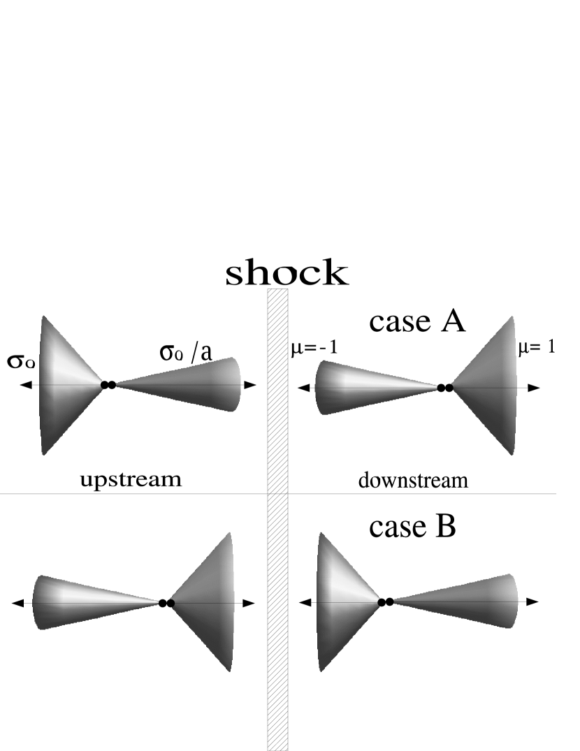
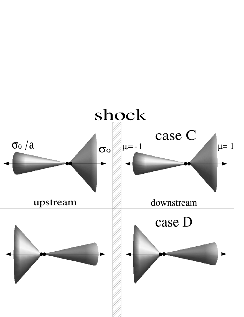
Figure 9: Pictorial representation of the four patterns of anisotropic scattering considered in our calculations.

In order to simulate the cases A-D above, we adopt a scattering function similar to Eq. (10), but modified to introduce anisotropic scattering. In particular, to achieve this goal we allow the width $\sigma$ of the scattering function to depend on both the initial and final directions $\mu^{\prime}$ and $\mu$, so that:

$$w(\mu,\mu^{\prime})={1\over\sigma(\mu,\mu^{\prime})}e^{-{1-\mu\mu^{\prime}\over\sigma(\mu,\mu^{\prime})}}I_{0}\left({\sqrt{1-\mu^{2}}\sqrt{1-\mu^{\prime 2}}\over\sigma(\mu,\mu^{\prime})}\right)\,.$$ (31)

It is worth stressing that the scattering function has to be symmetric if we exchange $\mu$ with $\mu^{\prime}$ as a consequence of Liouville’s theorem, so we are forced to look for a symmetric function $\sigma(\mu,\mu^{\prime})$.

In order to apply the functional form Eq. (31) to the cases A-D, it is sufficient to adopt the following expression for the mean scattering angle $\sigma(\mu,\mu^{\prime})$:

$$\sigma_{\mp}(\mu,\mu^{\prime})=\sigma_{\circ}\cdot\left(1-{(a-1)\over 4a}(\mu\mp 1)(\mu^{\prime}\mp 1)\right)\,.$$ (32)

Both $\sigma_{+}$ and $\sigma_{-}$ have $\sigma_{0}$ as the maximum and $\sigma_{\circ}/a$ as the minimum value. For this reason we will refer to $a$ as the Anisotropy Factor. For $a=1$, isotropic scattering is recovered.

The resulting scattering function $w_{\mp}(\mu,\mu^{\prime})$, obtained substituting Eq. (32) into (31), is plotted in Fig. 10 together with the isotropic scattering function (Eq. (10)), for $\sigma_{\circ}=0.05$ and $a=10$. These plots clarify how $w_{+}$ and $w_{-}$ can simulate a scattering more efficient in the $\mu=+1$ and $\mu=-1$ directions respectively.

Figure 10: The thick lines show the anisotropic scattering functions $w_{+}(\mu,\mu_{\circ})$ (left box) and $w_{-}(\mu,\mu_{\circ})$ (right box), as functions of $\mu$ and for different values of the incoming direction $\mu_{\circ}$. The anisotropy factor is $a=10$ and $\sigma_{\circ}=0.05$. For comparison the isotropic scattering function (Eq. (10)) is shown with thin lines and for the same values of $\mu_{\circ}$.

The condition $\int_{-1}^{1}d\mu\,w(\mu,\mu^{\prime})=1$ that states the probability conservation, is fulfilled by Eq. (31) provided $\sigma_{0}\ll 1$. In the numerical calculations that follow we assume $\sigma_{0}=0.05$.

Using $\sigma_{-}$ and $\sigma_{+}$ in different combinations for the upstream and the downstream fluids, we can reproduce scenarios A, B, C, and D, as summarized in Table 2.

Table 2: Summary of mean scattering angle used in the different scenario of fig.9.

	$A$	$B$	$C$	$D$
upstream	$\sigma_{+}$	$\sigma_{-}$	$\sigma_{-}$	$\sigma_{+}$
downstream	$\sigma_{-}$	$\sigma_{+}$	$\sigma_{-}$	$\sigma_{+}$

4.2 Results: anisotropic scattering for shocks of arbitrary speed and fixed anisotropy factor

Following the procedure outlined in §2 and making use of Eqs. (31) and (32), we compute the spectral index and the angular distribution for the scenarios A, B, C and D, described above. In each case both the parameter $\sigma_{\circ}$ and the anisotropy factor $a$ are fixed ($\sigma_{\circ}=0.05$ and $a=10$), while the shock velocity is allowed to vary within the range $0.04\leqslant\Gamma_{s}\beta_{s}\leqslant 5$.

The angular part of the distribution function is shown in Fig. 11 for the scenarios A (left panel) and B (right panel) and in Fig. 12 for the scenarios C (left panel) and D (right panel). The slope of the spectrum of accelerated particles is plotted in Fig. 13.

Figure 11: Particle distribution function at the shock front for anisotropic scattering of type A (on the left) and B (on the right) both with $a=10$. Each line represents a different shock speed as the labels show.

Figure 12: The same as fig.11 but for anisotropic scattering of type C (on the left) and D (on the right).

Figure 13: Slope vs. shock speed in the four different anisotropic scattering scenarios: A and B in the left box, C and D in the right one. All plots are obtained with $a=10$ and $\sigma_{0}=0.05$. Slope resulting from isotropic scattering (computed with $\sigma=0.01$) is also shown for comparison (solid line).

For relativistic shocks, the spread in the slope of the spectrum of accelerated particles has less spread around $\sim 4$, although in general it remains true that harder spectra are obtained in the scenarios B and D.

A note of caution is necessary to interpret the apparent peak in the slopes at $\Gamma_{s}\beta_{s}\sim 1$ for cases A, and at $\Gamma_{s}\beta_{s}\sim 3$ for cases D. These peaks are completely unrelated to anisotropic scattering and is instead the result of the breaking of the regime of small pitch angle scattering (or SPAS), as was already pointed out in Blasi $\&$ Vietri (2005). The acceleration process does no longer take place in the SPAS regime when $\Gamma_{s}^{2}\gtrsim 1/4\sigma$, which happens at higher Lorentz factor when $\sigma$ is smaller. This is shown in Fig. 14, where we plot the slope for the case of isotropic SPAS for $\sigma=0.1$ (dashed line) and $\sigma=0.01$ (solid line), and the corresponding angular distribution for $\Gamma_{s}\beta_{s}=5$. As already found in Blasi $\&$ Vietri (2005), the transition from SPAS to LAS is generally accompanied by a hardening of the spectra of accelerated particles. The peak seen in Fig. 13 is simply the consequence of an effective value of $\sigma$ in the anisotropic scattering cases A and D. This is also clear comparing angular distributions of Fig. 14 with the angular distribution of cases A and D for $\Gamma_{s}\beta_{s}=4$ and 5: the curves show the same behaviour with a jump at $\mu=-\beta_{\rm down}$ and a peak that moves towards $\mu=1$ as the shock speed increase.

Figure 14: These plots show the breaking of the SPAS approximation. Left box: slope of the spectrum of accelerated particles in the case of isotropic scattering with $\sigma=0.01$ (solid line) and $\sigma=0.1$ (dashed line). Right box: angular distribution for $\Gamma_{s}\beta_{s}=5$ with $\sigma=0.01$ (solid line) and $\sigma=0.1$ (dashed line).

5 Conclusions and Discussion

In this paper we carried out exact calculations of the angular distribution function and spectral slope of the particles accelerated at plane shock fronts moving with arbitrary velocity, generalizing a method previously described in detail in Vietri (2003); Blasi $\&$ Vietri (2005). In particular, we specialized our calculations to two situations: 1) presence of a large scale coherent magnetic field of arbitrary orientation with respect to the shock normal, in the upstream fluid; 2) possibility of anisotropic scattering in the upstream and downstream plasmas.

Our calculations allowed us to describe the importance of the inclination of the magnetic field when this has a large coherence length and there are no scattering agents upstream. For newtonian shocks, only quasi-perpendicular fields (namely perpendicular to the shock normal) are of practical importance, in that the return of particles to the shock from the upstream section is warranted. Quasi-parallel shocks imply a very low probability of return, so that the spectrum of accelerated particles is extremely soft. The process of acceleration eventually shuts off for parallel shocks. For relativistic shocks, the situation is less pessimistic because the accelerated particles and the shock front move with comparable velocities in the upstream frame. In general, the acceleration stops being efficient when the cosine of the inclination angle $\alpha$ of the magnetic field with respect to the shock normal is comparable with the shock speed in units of the speed of light. The slope of the spectrum of accelerated particles for $\cos\alpha=0$ as a function of the shock velocity is plotted in Fig. 6 for the two cases in which SPAS or LAS is operating in the downstream plasma. The slope as a function of $\cos\alpha=0$ for shocks moving at different speeds is shown in Fig. 8. In the same figure we also show the return probability from the upstream section, in order to emphasize that the presence of a large scale magnetic field upstream leads to particle leakage to upstream infinity. This latter phenomenon disappears when scattering is present, in that scattering always allows for the shock to reach the accelerated particles. In this case the probability of returning to the shock at an arbitrary direction is unity. One can ask when and how the transition from a situation in which there is no scattering to one in which scattering is at work takes place. When some scattering is present but the energy density in the scattering agents (e.g. Alfvèn waves) is very low compared with the energy density in the background magnetic field, only very low energy particles are effectively scattered. When their energy becomes large enough, they only feel the presence of the coherent field. Increasing the amount of scattering, this transition energy becomes gradually higher. Particles whose Larmor radius is larger that the coherence scale of the magnetic field can eventually escape the accelerator. In general the level of turbulence (and therefore of scattering) and the number of accelerated particles are not independent since the turbulence may be self-generated through streaming-like instabilities Bell (1978).

In §4 we extended our analysis to the very interesting case of anisotropic scattering in both the upstream (unshocked) and downstream (shocked) medium. The pattern of anisotropy, which clearly depends on the details of the formation and development of the scattering centers, has been parametrized in four different scenarios, and for each one we calculated the angular part of the distribution function and the spectrum of the accelerated particles. Deviations from the predictions obtained in the context of isotropic SPAS and LAS have been quantified: the typical magnitude of these deflections is a few percent, but there are situations in which the deviation is more interesting, in particular because it goes in the direction of making spectra harder.

References

- Achterberg et al. (2001) Achterberg, A., Gallant, Y.A., Kirk, J.G., Guthmann, A.W., 2001, MNRAS, 328, 393.
- (2) Ballard, K.R., Heavens, A.F., 1991, MNRAS, 251, 438.
- Bednard Ostrowski (1998) Bednard, J., Ostrowski, M., 1998, Phys. Rev. Lett., 80, 3911. arXiv:astro-ph/9806181 v1.
- Bell (1978) Bell, A.R., 1978, MNRAS, 182, 147.
- Blasi Vietri (2005) Blasi, P., Vietri, M., 2005, ApJ, 626, 877.
- Freiling, Vietri Yurko (2003) Freiling, G., Vietri, M., Yurko, V., 2003, Letters in math. Phys., 64, 65.
- Gallant (2002) Gallant, Y.A., 2002, Relativistic flow in Astrophysics, Lecture Notes in Physics, 589, pp. 24-40. arXiv:astro-ph/0302231.
- Gallant Achterberg (1999) Gallant, Y.A., Achterberg, A., 1999, MNRAS, 305, L6.
- Kirk et al. (2000) Kirk, J.G., Guthmann, A.W., Gallant, Y.A., Achterberg, A., 2000, arXiv:astro-ph/000522 v2.
- Kirk Duffy (1999) Kirk, J.G., Duffy, P., 1999, J. Phys. G., 25, R163. arXiv:astro-ph/9905069 v1.
- Kirk Schneider (1987) Kirk, J.G., Schneider, P., 1987, ApJ, 315, 425
- Lemoine Pelletier (2003) Lemoine, M., Pelletier, G., 2003, ApJ, 589, L73. arXiv:astro-ph/0304058 v2.
- Lemoine Revenu (2005) Lemoine, M., Revenu, B., 2005, MNRAS, 000, 1. arXiv:astr-ph/0510522 v1.
- Niemiec Ostrowski (2004) Niemiec, J., Ostrowski, M., 2004, ApJ, 610, 851
- Synge (1957) Synge, J.L., 1957, The relativistic gas, North-Holland, Amsterdam.
- Peacock (1981) Peacock,J. A., 1981, MNRAS, 196, 135.
- Vietri (2003) Vietri, M., 2003, ApJ, 591, 954.