Energetics of solar coronal mass ejections

Abstract

Aims. We investigate whether solar coronal mass ejections are driven mainly by coupling to the ambient solar wind or through the release of internal magnetic energy.

Methods. We examine the energetics of 39 flux-rope like coronal mass ejections (CMEs) from the Sun using data in the distance range $\sim$ 2–20 $R_{\odot}$ from the Large Angle Spectroscopic Coronograph (LASCO) aboard the Solar and Heliospheric Observatory (SOHO). This comprises a complete sample of the best examples of flux-rope CMEs observed by LASCO in 1996-2001.

Results. We find that 69% of the CMEs in our sample experience a clearly identifiable driving power in the LASCO field of view. For the CMEs that are driven, we examine if they might be deriving most of their driving power by coupling to the solar wind. We do not find conclusive evidence in favor of this hypothesis. On the other hand, we find that their internal magnetic energy is a viable source of the required driving power. We have estimated upper and lower limits on the power that can possibly be provided by the internal magnetic field of a CME. We find that, on average, the lower limit to the available magnetic power is around 74% of what is required to drive the CMEs, while the upper limit can be as much as an order of magnitude larger.

1 Introduction

The basic energetics of coronal mass ejections (CMEs) from the Sun is a subject of intense research. The amount of energy required to disrupt initially closed magnetic field lines and to lift and accelerate CMEs against the gravitational field of the Sun are key ingredients of CME initiation models (e.g., Amari et al. 2000; Antiochos, DeVore & Klimchuk 1999; Forbes 2000). While the energetics of CMEs in the lower corona is poorly understood, the energetics of CMEs beyond $\sim$ 2R_⊙ is somewhat better understood (Vourlidas et al. 2000; Vourlidas et al. 2002; Lewis & Simnett 2002). Since the advent of the excellent dataset of CMEs provided by the Large Angle Spectroscopic Coronograph (LASCO, Brueckner et al. 1995) aboard the Solar and Heliospheric Observatory (SOHO, Domingo et al. 1995), there have been only a few papers that have examined the energetics of several CMEs. Vourlidas et al. (2000) (Paper 1 from now on) studied the evolution of the potential, kinetic, and magnetic energies of 11 flux-rope CMEs in an attempt to understand the driving mechanism for such CMEs beyond $\sim$ 2R_⊙. They surmised that the energy contained in the magnetic fields advected by the CMEs could be responsible for propelling them. Some recent studies of the initiation of flux-rope CMEs (Amari et al. 2000) suggest that $\sim$ 55% of the available magnetic free energy could be available for propagating the CME through the corona.

On the other hand, Lewis & Simnett (2002) used an ingeneous method to study the weighted average profile of all the CMEs in the LASCO C2 and C3 fields of view from March 1999 to March 2000 to investigate similar questions. They found that the mechanical (i.e., kinetic + potential) energy of a typical CME in this period increased with time at a remarkably constant linear rate as it propagated through the LASCO C2 and C3 fields of view. Based on this constant rate of input power to a typical CME, they concluded that CMEs are likely to be powered by momentum coupling with the solar wind, which is an effectively infinite energy reservoir for most CMEs. It may be noted that they did not measure individual CMEs to arrive at this conclusion, nor did they present adequate calculations to support it. It is therefore an aggregate statement and, as we will see later, an incorrect one. In contrast, our method, which is outlined in § 2, involves detailed measurements of each CME in our sample. Manoharan (2006) has studied the evolution of 30 large Earth-directed CMEs by combining data from LASCO with that from the Ooty Radio Telescope (ORT). His dataset spans distances from $\sim$ 2 $R_{\odot}$–1 AU. He notes that the average CME in his sample arrives at the Earth around 13 hours sooner than a typical parcel of solar wind would, and thereby concludes that CMEs are not simply dragged along by the solar wind; they have to be driven by the expenditure of some kind of internal energy. However, the CMEs in his sample slow down significantly at distances $>$ 80 $R_{\odot}$. This suggests that the solar wind might be influencing CME propagation significantly for $R>80R_{\odot}$.

In this work, we concentrate on flux-rope (FR) CMEs because (i) flux-ropes are commonly invoked by several current theoretical and numerical models of CMEs (e.g., Chen 1996; Kumar & Rust 1996; Gibson & Low 1998; Birn, Forbes & Schindler 2003; Kliem & Török 2006) and (ii) their physical parameters can be derived by in-situ observations (e.g., Burlaga 1988; Lepping et al 1990; Hu and Sonerup 1998; Mulligan and Russel 2001; Lynch et al. 2003; Lepping et al 2003). Generally, LASCO observes many events sufficiently structured to be characterized as FR CMEs under some viewing assumptions (e.g., Cremades and Bothmer 2004). In Paper 1 and here, we have adopted a much stricter definition for a FR CME; namely, the event must exhibit a clear circular structure with visible striations in its core. In other words, the CME must closely resemble the cross section of a theoretical flux-rope (also see § 3.2). Based on this criterion, we study the evolution of potential and kinetic energies of 39 individual FR CMEs between 1997 and 2001. This comprises a complete sample of the best examples of FR CMEs observed by LASCO in 1996-2001 (out of about 4000 events). In doing so, we obtain better statistics than Paper 1 and include a wider variety of events through the rising phase and maximum of cycle 23. We find that the mechanical energy (i.e., kinetic + potential energy) of 69% of the events increases linearly with time. This implies that these events are clearly “driven” by the release of some sort of energy. Based on our examination of these individual events, we investigate if the CMEs could be powered by coupling to the solar wind. We also examine whether the release of the internal magnetic energy of a CME can account for its driving power.

2 Data analysis

2.1 Mass images

We have compiled a complete list of all CMEs that appear like flux ropes in the LASCO data between February 1997 and March 2001 and selected the best cases based on their morphological appearance in coronograph images for this study. The Thomson scattering process by which free electrons in the CME scatter photospheric light and give rise to these intensity images has a rather sharp dependence on the scattering angle. Those CMEs that retain their overall morphology in LASCO images are therefore probably ones that remain in the plane of the sky throughout these fields of view (Cremades and Bothmer 2004; also see § 3.2). Since the calculations of CME mass (see Paper 1) assumed that the CME is in the plane of the sky, this lends credence to our estimates of CME mass and velocity.

We now briefly describe the procedure we followed in order to obtain the evolution of CME energy from a time sequence of these intensity images. The intensity of Thomson-scattered light depends directly on the column density of coronal electrons off of which the scattering takes place. By backtracking through the Thomson scattering calculations, we are thus able to construct mass images from the observed intensity images. Each pixel of the mass image gives the surface density (g cm^-2) of coronal electrons. By subtracting a suitable pre-event (or, in some cases, post-event), mass image from the image containing the CME, we obtain an image that gives the excess mass (over the background corona) carried by the CME. We circumscribe the extent of the flux-rope structure within the CME as evident in the image and get its total mass by simply summing the masses of all the pixels comprising the CME. It is also straightforward to obtain the center of mass for the flux-rope structure of the CME from such a mass image, since we know the mass contained in each pixel and its spatial co-ordinates. A time sequence of these mass images gives the evolution of CME mass and the velocity of the center of mass. The time evolution of kinetic and potential energies of the CME are calculated from these quantities. This part of the data analysis procedure is similar to what is used in Paper 1, and we refer the reader there for further details.

Figure 1: The mechanical (i.e., kinetic + potential) energy for two representative CMEs plotted as a function of time from initiation. The mechanical energy for the CME on 2000/03/22 (upper panel) increases linearly with time, implying that there is a constant driving power on the CME as it propagates outwards. Such CMEs are included in category A (Table 1). The mechanical energy for the CME on 1998/08/13 (lower panel) shows no such trend. Such CMEs are included in category B (Table 2).

2.2 Driving power

Having obtained the time evolution of the kinetic and potential energies of a CME, we add them together to obtain the time evolution of its mechanical (i.e., kinetic + potential) energy. We find that for 27 CMEs, the mechanical energy rises linearly with time (category A, Table 1), whereas 12 CMEs show no such trend (category B, Table 2). In other words, 27 out of 39 CMEs (69%) belong to category A, whereas the remaining 12 (31%) CMEs belong to category B. The upper panel of figure 1 shows an example of a CME in category A (Table 1), where the linear rise of mechanical energy with time is clearly evident. The lower panel of figure 1 shows an example of a CME in category B (Table 2).

Table 1: Category A: CMEs for which Mechanical Energy increases linearly with time

Date	Time	PA	Speed	At Radius	Mass	Eruptive Prominence
		$\degr$	(km/s)	(R⊙)	($\times 10^{15}$ g)
97/11/01	20:11	271	275	20	1	Y
97/11/16	23:27a	85	595	20.5	5	N
98/02/04	17:02	289	425	19.5	5	N
98/02/24	07:28	90	500	19	1	N
98/05/07	11:05	270	450	21	10	N
98/06/02	08:08	245	600	14.5	10	Y
99/07/02	17:30	39	220	16.5	5	Maybe
99/08/02	22:26	271	380	24	2.5	Y
00/03/22	04:06	323	350	14	5	Maybe
00/05/05	07:26	338	260	9	1	N
00/05/29	04:30	278	178	10	1.5	Maybe
00/06/06	04:54	359	400	15	4	Y
00/06/08	17:07	59	310	10.5	2	N
00/07/23	17:30	14	400	9	1	N
00/08/02	17:54	46	700	20	7	Y
00/08/03	08:30	302	620	18	6	Y
00/09/27	00:50	327	455	15	1	N
00/10/26	00:50	99	200	12.5	2	Maybe
00/11/12	09:06	329	282	15	2	N
00/11/14	16:06	258	500	20	2	N
00/11/17	04:06	75	450	18	3	Y
00/11/17	06:30	188	500	18	3	Y
01/01/07	04:06	298	550	17	3	Y
01/01/19	17:06	78	900	18	3	Maybe
01/02/10	23:06a	229	900	23	4	Y
01/03/01	04:06	292	400	20	1	Maybe
01/03/23	12:06	284	400	15	7	N

• The time refers to the previous day.

• Column 1: Date on which a given CME occurred; Column 2: Start time in the C2 field of view; Column 3: central position angle of the CME (CCW from solar north); Column 4: Speed of the CME at the radius quoted in column 5; Column 5: This is the farthest radius until which we have been able to track the CME; Column 6: Mass of the CME at the radius quoted column 5. For instance, the CME on 97/11/01 has a speed of 275 km/s and a mass of $10^{15}$ g at 20 R_⊙; Column 7: Denotes whether or not the CME was associated with a prominence eruption (see § 3.4); ‘Y’ denotes that the CME was associated with a prominence eruption, ‘N’ denotes the converse and ‘Maybe’ denotes a situation where we are not certain that a prominence eruption was associated with the CME.

Table 2: Category B: CMEs for which mechanical energy remains constant with time

Date	Time	PA	Speed	At Radius	Mass	Eruptive Prominence
		($\degr$)	(km/s)	(R⊙)	($\times 10^{15}$ g)
97/02/23	02:55	82	910	15.5	1	Y
97/04/13	16:12	269	510	24	0.8	Y
97/04/30	04:50	84	330	18.5	0.7	N
97/08/13	08:26	273	350	20	1	N
97/10/19	04:42	92	260	11	1	Y
97/10/30a	18:21	88	225	17.5	1	N
97/10/31	09:30	262	410	23	1	N
99/05/23	07:40	288	600	30	1	N
99/07/04	21:54a	89	181	16	2	Maybe
00/11/04	01:50	213	794	29	3	Y
01/01/19	12:06	74	403	17	1	N
01/03/22	05:26	255	377	14.5	2	Y

• The time refers to the previous day.

• Columns same as Table 1.

For the CMEs in category A (Table 1), we fit a straight line to the plot of mechanical energy vs. time. The slope of this straight line gives the driving power. As pointed out in paper 1 (also see Vourlidas 2004, Lugaz et al. 2005) the mass of a given CME can be underestimated by at most a factor of 2. Furthermore, this would be a systematic error in the mass estimate for a given CME. It does not affect the slope of the mechanical energy vs. time curve for a given CME. The errors $\sigma_{D}$ on the values of the driving power thus arise only from the errors in determining the slope of the straight line fit. Column 2 of Table 3 gives the driving power $P_{D}$ determined in this manner and column 3 of Table 3 gives the associated error $\sigma_{D}$ for each CME in category A. Both these quantities are expressed in units of $10^{30}$ erg/hr.

2.3 Estimate of magnetic power

The driving power could be provided by the release of the internal magnetic energy of the FR CMEs. In order to estimate the power that can possibly be released by magnetic fields advected with an expanding CME, we need to know the magnetic field advected with the CME.

2.3.1 Direct estimate of magnetic fields carried by CMEs

Measurements of the coronal magnetic field (much less so for the magnetic field entrained by CMEs) are few and far between. Using radio measurements of what is presumably synchrotron emission from electrons populating the CME structure, Bastian et al. (2001) have estimated the magnetic field in a CME on 1998 April 20 to be $\sim$ 0.1 – 1 G. We adopt the value of 0.1G as a working figure for our purposes.

The magnetic energy contained in the CME can be written as

$$\widetilde{E_{M}}=\frac{B^{2}}{8\,\pi}\,l\,A\,,$$ (1)

where $B$ is the magnetic field, $A$ the cross-sectional area of the CME, and $l$ its length perpendicular to the plane of the sky. We measure $A$ directly for each CME (in each image), and we take $l$ to be equal to the heliocentric distance of the CME center of mass (in each image). The assumption for $l$ implies a reasonable flux rope length of one solar radius at the solar surface. The power ($\widetilde{P_{M}}$) that can possibly be released by the advected magnetic field is

$$\frac{d}{dt}\,\widetilde{E_{M}}=\widetilde{P_{M}}=\frac{B^{2}}{8\,\pi}\,\frac{d}{dt}\,l\,A\,.$$ (2)

Note that we have not accounted for the temporal variation of the magnetic field $B$ in computing $\widetilde{P_{M}}$. We use a conservative value of 0.1 G for the magnetic field $B$ and fit a straight line to the time evolution of $l\,A$ to get the values of $\widetilde{P_{M}}$ shown in column 8 of Table 3. The associated error $\widetilde{\sigma_{M}}$ quoted in column 9 of Table 3 arises only from the error $\sigma_{l\,A}$ in the straight line fit to the time evolution of $l\,A$. The quantity $\widetilde{\sigma_{M}}$ is defined as

$$\widetilde{\sigma_{M}}=\frac{B^{2}}{8\,\pi}\,\sigma_{l\,A}\,.$$ (3)

The quantities $\widetilde{P_{M}}$ and $\widetilde{\sigma_{M}}$ are expressed in units of $10^{30}$ erg/hr in table 3. Since we do not account for the possible decrease in the advected magnetic field as the CME propagates outwards, $\widetilde{P_{M}}$ is an upper limit on the power that can possibly be provided by its dissipation.

2.3.2 Magnetic flux carried by near-Earth magnetic clouds

On the other hand, magnetic clouds observed by near-Earth spacecraft are thought to be near-Earth manifestations of CMEs that are directed towards the Earth (e.g., Webb et al. 2000; Berdichevsky et al. 2002; Manoharan et al. 2004). We envisage a scenario where some of the magnetic flux carried by a CME is expended in driving it; what is left when it arrives at the Earth is detected by in-situ measurements of the corresponding near-Earth magnetic cloud. We can compute the magnetic power by assuming that the CME carried the same amount of magnetic flux near the Sun as what is observed in the near-Earth magnetic cloud. Such a calculation will necessarily yield a lower limit on the power that can be expended by the advected magnetic field in driving the CME.

Since the CMEs in our sample propagate primarily along the plane of the sky, they will not be detected as near-Earth magnetic clouds. However, Lepping et al. (1997) estimate the average magnetic flux carried by 30 well observed magnetic clouds to be $\overline{B.A}=10.8\times 10^{20}$ Mx, with a standard deviation error of $\sigma_{BA}=8\times 10^{20}$ Mx. The value of $\sigma_{BA}$ they quote is representative of the range of fluxes carried by different magnetic clouds and not of the errors in individual measurements. The actual fit error for $B$ and $A$ is approximately $6-7\%$ (Lepping et al. 2003); it is insignificant in comparison to the overall flux variation, $\sigma_{BA}$. If we assume that $\overline{B.A}$ is representative of the magnetic flux carried by the CMEs in our sample, we can write the following expression for the CME magnetic energy:

$$E_{M}=\frac{1}{8\,\pi}\,\frac{l}{A}\,(\overline{B.A})^{2}\,,$$ (4)

where $l$ and $A$ are the length and cross-sectional area of the flux rope, respectively. We take $l$ equal to the heliocentric distance of the CME as we did in (1). Consequently, a lower limit on the power derived from the decrease in magnetic energy as the flux rope expands outwards is given by

$$P_{M}=\frac{d}{dt}\,E_{M}=\frac{1}{8\,\pi}\,(\overline{B.A})^{2}\,\frac{d}{dt}\,\frac{l}{A}\,.$$ (5)

We have information about the time derivative of the quantity $l/A$ for each of the CMEs in our sample. The values of $P_{M}$ are quoted in column 4 of Table 3 in units of $10^{30}$ erg/hr for the CMEs in category A; i.e., the ones that show clear evidence of a driving power. The quantity $\sigma_{M}$ quoted in column 5 of Table 3 is the error in the value of the magnetic power, expressed in units of $10^{30}$ erg/hr. The error $\sigma_{M}$ in the value of the magnetic power arises from the error $\sigma_{BA}$ in the average magnetic flux and the error $\sigma_{l/A}$ in fitting a straight line to the time evolution of $l/A$. The error in the value of $\overline{B.A}^{2}$ is related to $\sigma_{BA}$ by $\sigma_{BA^{2}}=2\,\,\overline{B.A}\,\,\sigma_{BA}$. The value of $\sigma_{M}$ is defined by

$$\sigma_{M}=P_{M}\sqrt{\biggl{(}\frac{\sigma_{BA^{2}}}{(\overline{B.A})^{2}}\biggr{)}^{2}+\biggl{(}\frac{\sigma_{l/A}}{\frac{d}{dt}\frac{l}{A}}\biggr{)}^{2}}\,$$ (6)

3 Results and Interpretation

As mentioned earlier, the mechanical energies of the 27 CMEs in category A (Table 1) increase linearly with time, implying a constant driving power for these CMEs. The mechanical energies for the 12 CMEs in category B (Table 2), on the other hand, show no such trend. Figure 1 shows an example from each category; the upper panel shows an example of a CME for which the mechanical energy increases linearly with time, implying a constant driving power, while the lower panel shows an example where there is no evidence for a linear increase of mechanical energy with time.

3.1 Source of driving power for CMEs from $\sim$ 2–20 $R_{\odot}$: solar wind or advected magnetic field?

Based on the constancy of power required to drive a typical CME, Lewis & Simnett (2002) surmise that CMEs could be driven via momentum coupling with the solar wind, which is an effectively infinite energy reservoir for the CMEs. However, they did not measure individual CMEs to arrive at this conclusion, but instead employed a weighted average method that gave this result for a typical CME between March 1999 and March 2000.

CMEs could be driven by the ambient solar wind via the hydromagnetic buoyancy force $F_{\rm solwind}$. We write the following expression for this force following eq (22) of Yeh (1995):

$$F_{\rm solwind}=\pi\,Q^{2}\,(-\,\nabla\,p_{\infty})\,,$$ (7)

where $\pi\,Q^{2}$ represents the cross-sectional area presented by the CME, and the term inside the brackets is the gradient in the ambient pressure that drives the solar wind. Evidently, if the driving force on a CME is predominantly due to coupling with the solar wind, it should be proportional to its cross-sectional area. We now take a closer look at the CMEs in category A (Table 1). Figure 2 is a scatterplot of the mechanical driving force versus mean CME size (measured in number of pixels) for these CMEs.

Figure 2: The mean size (in number of pixels) for the CMEs in category A (Table 1) plotted as a function of their driving force. The low correlation coefficient suggests that there is no evidence to claim that larger CMEs have greater driving forces (see § 3.1).

We calculate the driving force by dividing the driving power for a CME (§ 2.2) by the velocity of its center of mass. The correlation between the driving force and CME size is evidently poor, and there is little evidence to suggest that larger CMEs experience a greater driving force. This casts doubt on the hypothesis that the CMEs in category A (Table 1) (which are clearly “driven”) are powered by coupling with the ambient solar wind.

On the other hand, several researchers have suggested that a combination of different kinds of Lorentz forces can drive the CME outward (e.g., Chen 1996; Kumar & Rust 1996). Most recently, Kliem & Török (2006), have investigated the interesting possibility of the so-called torus instability being responsible for driving the CME. This instability relies on the interplay between the Lorentz self-force in the torus-like CME structure and the opposing Lorentz force due to the ambient magnetic field.

We therefore turn our attention to the CME magnetic field to see if it can act as a driver. In view of the considerable uncertainties in determining coronal magnetic fields, we computed upper and lower limits on the rate of energy released by the magnetic field advected by each CME. The procedures we adopted are explained in § 2.3.1 and § 2.3.2. We computed the magnetic powers only for the CMEs in category A (Table 1), which are evidently driven.

Table 3: Driving power and magnetic power for Category A

Date	$P_{D}$	$\sigma_{D}$	$P_{M}$	$\sigma_{M}$	$P_{M}$/$P_{D}$	$\sigma_{P_{M}/P_{D}}$	$\widetilde{P_{M}}$	$\widetilde{\sigma_{M}}$	$\widetilde{P_{M}}$/$P_{D}$	$\sigma_{\widetilde{P_{M}}/P_{D}}$
97/11/01	0.229	0.022	0.620	0.925	2.708	4.032	5.872	0.667	25.583	2.904
97/11/16	2.426	0.198	0.287	0.431	0.118	0.712	24.548	2.595	10.117	1.069
98/02/04	1.477	0.158	0.336	0.505	0.228	0.583	10.945	0.132	7.410	0.897
98/02/24	0.306	0.077	0.511	0.758	1.668	2.480	6.642	0.808	21.686	2.639
98/05/07	3.295	0.355	0.494	0.739	0.150	0.751	8.145	1.554	2.471	0.473
98/06/02	7.274	0.656	0.718	1.086	0.098	0.926	23.054	3.809	3.169	0.524
99/07/02	0.835	0.127	0.187	0.278	0.224	0.757	18.826	3.061	22.550	3.667
99/08/02	0.478	0.023	0.324	0.481	0.678	1.009	7.200	0.682	15.053	1.425
00/03/22	1.060	0.017	0.312	0.463	0.295	0.441	3.147	0.409	2.975	0.387
00/05/05	0.358	0.038	1.120	1.665	3.122	4.646	1.324	0.160	3.693	0.447
00/05/29	0.488	0.052	0.528	0.783	1.082	1.608	2.311	0.274	4.733	0.562
00/06/06	1.153	0.031	0.659	0.979	0.572	0.851	4.750	0.622	4.121	0.539
00/06/08	0.705	0.095	0.840	1.269	1.190	1.802	9.941	1.364	14.088	1.933
00/07/23	0.747	0.208	0.740	1.106	0.989	1.505	3.566	0.581	4.770	0.780
00/08/02	3.557	0.099	0.562	0.843	0.158	0.295	28.542	3.970	8.025	1.115
00/08/03	3.789	0.200	0.839	1.271	0.221	0.411	30.443	4.224	8.035	1.115
00/09/27	0.805	0.100	0.433	0.654	0.540	0.844	17.342	2.020	21.550	2.510
00/10/26	0.224	0.020	0.196	0.291	0.874	1.301	1.771	0.246	7.890	1.095
00/11/12	1.187	0.041	0.410	0.611	0.346	0.525	8.740	0.804	7.361	0.678
00/11/14	0.630	0.075	0.890	1.348	1.408	2.140	20.874	2.654	33.104	4.210
00/11/17	1.120	0.029	0.747	1.117	0.668	1.001	9.486	1.241	8.487	1.110
00/11/17	0.826	0.050	0.695	1.031	0.841	1.251	8.843	1.806	10.710	2.188
01/01/07	1.372	0.089	0.633	0.960	0.461	0.714	22.125	3.517	16.124	2.563
01/01/19	2.630	0.256	0.792	1.182	0.301	0.554	15.580	2.970	5.930	1.130
01/02/10	2.744	0.380	0.103	0.154	0.037	3.685	68.621	8.920	25.007	3.250
01/03/01	0.481	0.048	0.381	0.569	0.792	1.190	22.470	2.450	46.700	5.086
01/03/23	1.766	0.063	0.577	0.859	0.326	0.498	11.900	1.660	6.740	0.941
Averages	1.554	0.130	0.553	0.828	0.744	1.352	14.704	1.970	12.819	1.677

• The numbers in columns $2-5$ and $8-9$ are expressed in units of $10^{30}$ erg/hr. Column 1: Date on which the CME occurred; Column 2: Driving power $P_{D}$ associated with a CME; Column 3: Error $\sigma_{D}$ associated with the driving power (§ 2.2); Column 4: Estimate of the magnetic power $P_{M}$ that could be released by the CME using an estimate of the magnetic field carried by near-Earth magnetic clouds; Column 5: Error $\sigma_{M}$ associated with this estimate (§ 2.3.1); Column 6: Ratio of $P_{M}$ to $P_{D}$; Column 7: Error associated with the quantity $P_{M}/P_{D}$; Column 8: Estimate of the magnetic power $\widetilde{P_{M}}$ that could be released by the CME using an estimate of the magnetic field entrained in the CME; Column 9: Error $\widetilde{\sigma_{M}}$ associated with this estimate (§ 2.3.2); Column 10: Ratio of $\widetilde{P_{M}}$ to $P_{D}$; Column 11: Error associated with the quantity $\widetilde{P_{M}}/P_{D}$.

The quantity $\widetilde{P_{M}}$ is an upper limit on the available magnetic power, and $\widetilde{\sigma_{M}}$ is the associated error(§ 2.3.1). These are listed in columns 8 and 9 of Table 3. Column 10 of Table 3 gives the ratio of $\widetilde{P_{M}}$ to the required driving power $P_{D}$ and column 11 gives the error associated with this quantity. The average of the numbers in column 10 is $12.819\pm 1.677$. We thus find that the upper limit on the available magnetic power could be as much as an order of magnitude greater than what is required to drive the CME. While this discrepancy might seem rather large, it may be noted that, besides driving the CME, part of the internal magnetic energy could also be expended in heating the plasma entrained in the CME (e.g., Kumar & Rust 1996) and in overcoming the “frictional drag” with the solar wind (e.g., Vrsnak et al. 2004; Cargill 2004). In-situ measurements of near-Earth magnetic clouds (Burlaga 1988; Lepping et al 1990; Hu and Sonerup 1998; Mulligan and Russel 2001; Lynch et al. 2003; Lepping et al 2003) reveal that there is an appreciable amount of magnetic flux left over after dissipation by these means.

The quantity $P_{M}$ is the lower limit on the available magnetic power and $\sigma_{M}$ is the associated error(§ 2.3.2). These are listed in columns 4 and 5 respectively of Table 3. Column 6 of Table 3 gives the ratio of $P_{M}$ to the required driving power $P_{D}$ and column 7 gives the error associated with $P_{M}/P_{D}$. The average of the numbers in column 7 is $0.74\pm 1.35$. We thus find that the lower limit on the available magnetic power is an appreciable fraction of what is needed to drive a representative CME in our sample. The lower limit on the available magnetic power is computed on the basis of the magnetic flux detected near the Earth. This magnetic flux represents the amount that is left over after driving the CME, heating it and overcoming the solar wind frictional drag. It is therefore significant that the driving power computed on the basis of this residual flux can still account for an appreciable fraction of what is needed to drive the CME.

3.2 Propagation effects and evolution of the white-light flux-rope structure

So far, we have been using the generic term “CME” to describe the properties of the flux-rope-like feature that is only a part of the overall CME phenomenon. It is implicit in our discussion that this feature comprises a well-defined structure, a system that could correspond to the flux-rope predicted/invoked in several CME models. In Paper 1, we suggested that the flux-rope CME propagates as an isolated system based on our findings of constant total energy for those events. This result supports the idea that the white-light signature of a flux-rope CME is indeed a flux-rope.

Perhaps we could get more clues to the nature of the flux-rope signature by looking into its dynamical evolution. If it is a flux-rope, we could expect small or no distortion of its shape as it propagates in the coronagraph field of view. We would also expect small correlation with the evolution of the other ejecta in the CME. The evolution of the flux-rope CME can be followed through the evolution of its center-of-mass. Figure 3 shows the front and center-of-mass height-time plots for four representative flux-rope CMEs in our sample. For about half of the events (18/39), the center-of-mass seems to closely track the evolution of the front. The events of 1997/04/13 and 1998/05/07 shown in Fig 3 are examples of such CMEs.

Figure 3: Representative front (stars) and center-of-mass (crosses) height-time plots for flux-rope CMEs. The event date is shown on each plot. The left side panels show events where the front and center-of-mass propagate with similar speeds and/or accelerations. The right side panels show events where the center-of-mass appears to decelerate relative to the CME front. See § 3.4 for further discussion.

For such CMEs, the flux-rope and the CME front propagate with similar velocities and no distortion of the flux-rope is observed. This result supports the idea that the white-light feature is indeed an isolated magnetic structure.

The events of 2000/03/22 and 2001/03/23 shown in Fig 3 are representative of the other half of our CME sample (19/39). For these CMEs, the center-of-mass seems to decelerate relative to the CME front as is evident from the diverging height-time curves. This is caused by a progressive center-of-mass shift towards the back of the flux-rope. The location of the center-of-mass is biased towards the location of the brightest pixels within the flux-rope structure. Thus, the shift of the center-of-mass is due to a brightness increase at the back of the flux-rope, which is equivalent to mass accumulation at that location. An inspection of the LASCO mass images supports our conclusion. It appears that the flux-rope structure of the CME propagates at a slower speed than the other ejecta coming behind the main CME structure (the post-CME coronal outflow) which results in the accumulation of mass at the back of the flux-rope. This is exactly what one would expect if the CME core is a low beta structure, a flux-rope, propagating in the solar wind flow. The same behavior has also been seen in 3D MHD models of erupting fluxropes (Lynch et al 2004). We believe that these observations strongly indicate that the white light “flux-rope”-like feature is indeed a magnetically closed structure; a flux-rope. We also suggest that the same effect is responsible for the so-called “disconnection” or “V-shaped” features mentioned often in the literature. In that case, only the back of the flux-rope is visible either because of the sensitivity of the instrument or because of the low density of the white-light flux-rope.

3.3 Association with prominences

In theories of filament formation (Karpen et al. 2003 and references therein), flux-rope structures are commonly associated with either the filament itself or with large-scale structures within which the filament lies. Most flux-rope models of CMEs also assume that prominence material is contained inside the flux-rope. It is therefore tempting to take the observations of flux-rope-like structures in white-light coronagraphs as evidence of the existence of flux ropes in the solar atmosphere, and look for the association of filament/prominence eruptions with these events. However, the relationship between pre-existing flux ropes and white-light CMEs is still unclear from an observational point of view. To see if our particular sample of CMEs can shed some light on this issue, we searched for evidence of eruptive prominence/filament associated with the CMEs we studied. We mainly used the EIT 195Å images because it is easier to correlate the LASCO/EIT databases. We also used the NOAA lists of active prominences/filaments, the Nobeyama radioheliograph database of limb events, and Big Bear H$\alpha$ movies where available. Our results are shown in column 7 of Table 1 and column 7 of Table 2. It was generally easy to discern whether a given event involved a prominence/filament eruption. For the events labeled “maybe”, we could see some filament motion or sprays of possibly cool material (the material appeared dark in the EUV images) but no clear evidence of large-scale filament/prominence ejection.

We find that 38% or 15/39 events have a clear association with an eruptive prominence/filament. A small number of the events (18% or 7/39) have some indication that chromospheric material was involved, but we cannot conclusively say whether a large-scale filament was indeed ejected. Almost half of the events (44% or 17/39) appear to have no association with a filament/prominence. This is a somewhat unexpected result. Given the close morphological resemblance of these white-light CMEs to flux-ropes, one would expect a closer correlation between filament eruption and flux-rope-like CMEs. There is always the possibility that filaments on the far side of the Sun could have been involved in the events for which we found no filament association on the visible side or that a filament channel did exist but without sufficient amounts of cold material to be detected in the images. Since we do not have any information on the conditions on the far side of the Sun, we relied solely on the available observations for the statistics. It might also be possible that these events are associated with active-region filaments that are generally harder to detect. To the extent we can tell from our current observations, we conclude that the flux-rope CMEs in our sample are not strongly correlated with filament eruptions. Our findings can be contrasted to those of Subramanian et al. (2001), who found that 59% of CMEs with signatures on the solar disk were associated with prominence eruptions.

3.4 Statistical properties of flux-rope CMEs

Finally, we can use our relatively large sample of events to derive statistical properties for the flux rope CMEs. We summarize these statistics in Fig 4. The distributions of mass and kinetic energies of the sample are shown in the top panels of Fig 4.

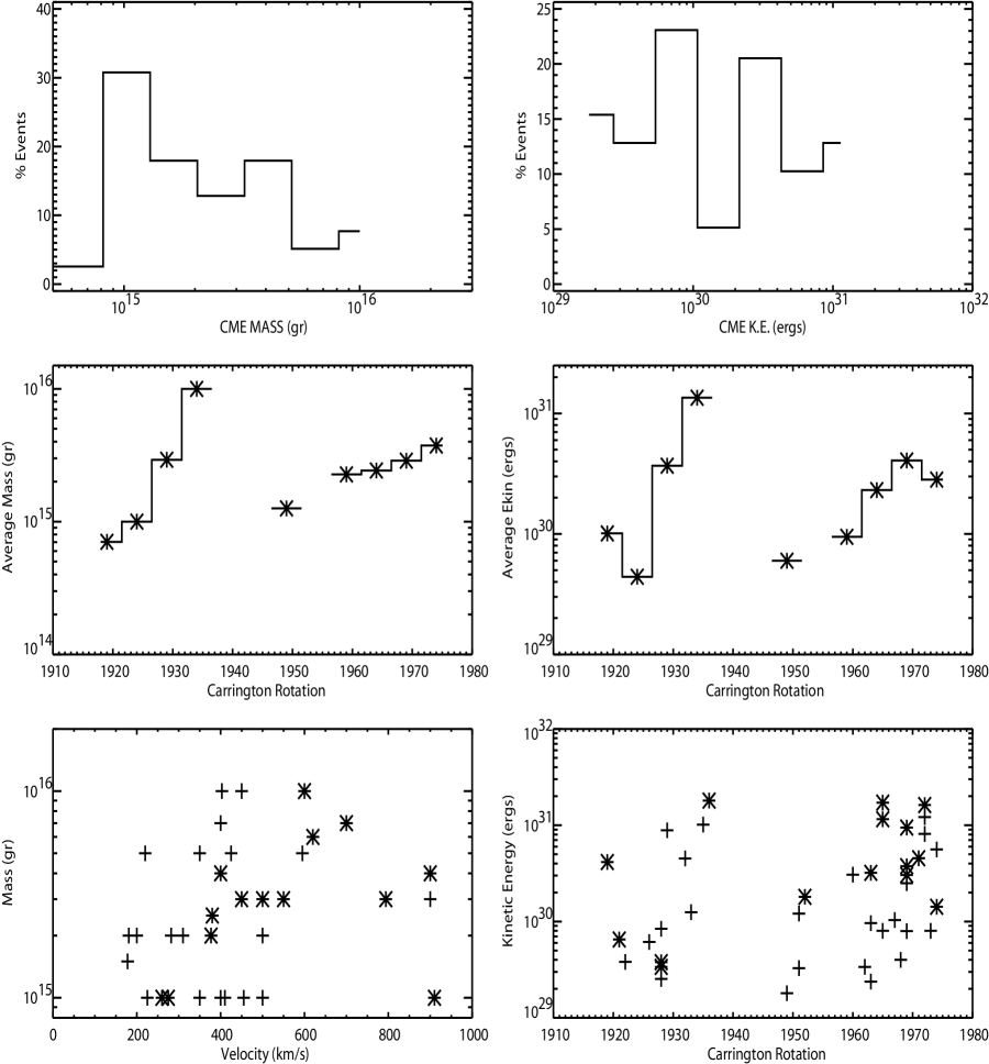
Figure 4: Statistics for our flux-rope CME sample. Top left: Histogram of CME masses. Top right: Histogram of CME kinetic energies. CME mass as a function of Carrington rotation (middle left) and CME kinetic energy as a function of Carrington rotation(middle right). The bins are averages over 5 rotations. Scattterplot of CME mass versus front speed (bottom left) and CME kinetic energy versus Carrington rotation (bottom right). The stars correspond to the events associated with eruptive prominences.

Flux-rope CMEs have an average mass of $3.1\times 10^{15}$ gr and an average kinetic energy of $4.1\times 10^{30}$ ergs. These numbers can be compared to $1.7\times 10^{15}$ gr and $4.3\times 10^{30}$ ergs for the average mass and kinetic energy for the whole sample of LASCO CMEs between 1996-2002 (Vourlidas et al. 2002). The middle panels of Fig 4 show the temporal variation of the mass and kinetic energy of flux-rope CMEs as a function of Carrington rotation. These numbers were calculated by averaging the measurements over 5 rotations. A sharp rise in mass and kinetic energy in 1998 (Carrington numbers 1935-1940) is evident despite the rather small number of events. A similar rise in the occurrence rate (Gopalswamy et al. 2003) and the average mass per event (Vourlidas et al. 2002) has been seen in the full sample of LASCO CMEs. Thus, the rise appears to be a real CME characteristic for this solar cycle. It is to be noted, however, that LASCO observations were severely disrupted in the last half of 1998 and early 1999 and that our statistics have not been corrected for duty cycle. On the other hand, a slower increase in the flux-rope CME properties since 1999 is also seen in larger CME samples (Vourlidas et al. 2002; Gopalswamy et al. 2003) and is probably real. Finally, we look at the properties of the flux-rope CMEs that are associated with filaments/prominences. The bottom panels of Fig 4 show the scatterplots of the mass and kinetic energy of the filament-associated CMEs (stars) and the rest of the sample (crosses). It is evident that filament-associated CMEs are slightly more energetic than the average CME event. Their average kinetic energy is $6.4\times 10^{30}$ ergs, almost 3 times higher than the average kinetic energy ($2.8\times 10^{30}$ ergs) of the total CME sample. The results are summarized in Table 4.

Table 4: Statistical properties of flux-rope CMEs

Sample	Average Width	Average Speed	Average Mass	Average Kinetic Energy
	(deg)	(km/s)	($10^{15}$ gr)	($10^{30}$ ergs)
Flux-rope CMEs	90	490	3.1	4.1
All LASCO CMEs	75a	417a	1.7b	4.3b

• For all CMEs in 1996-2001 (Yashiro et al. 2004)

• For all CMEs in 1996-2001 (Vourlidas et al. 2002)

4 Discussion and conclusions

We have examined the complete archive of LASCO observations between 1996-2001 and selected the best examples of CMES with a clear flux-rope structure (39 events). Our measurements suggest that the “flux-rope”-like structure in the core of these events does indeed behave as an isolated system, as one would expect from a magnetic structure (§ 3.4). Overall, we find that only 38% of these flux rope CMEs are unambiguously correlated to prominence eruptions (§ 3.3) which is somewhat suprising given the widely-held notion that the flux-rope appearance originates from the filament or the cavity above it. This observation does not preclude the possibility that a filament channel existed without detectable amounts of prominence material.

We studied the evolution and energetics of the flux rope structure for these 39 FR CMEs at heights $\sim 2$ R_⊙–20 R_⊙. We find that 69% of the CMEs in our sample experience a clear driving power in the LASCO field of view (§ 2.2). We find no evidence to suggest that these CMEs derive their driving power primarily via coupling with the solar wind in the range 2–20 R_⊙. If this was so, the driving force on the CME would be directly proportional to its cross sectional area (Eq 4). However, a scatterplot of driving force on a CME versus its mean cross sectional area reveals no such trend (Fig 2). On the other hand, several models for CME propagation rely on different kinds of Lorentz forces, which ultimately result in the dissipation of its internal magnetic energy. To investigate whether the release of the internal magnetic energy in the CME can possibly provide this driving power, we adopted two methods. We first used magnetic field measurements obtained from radio observations of a CME at around 2 R_⊙. In computing the available magnetic power using this method, we do not account for the possible decrease of this magnetic field as the CME propagates outwards (Eq 2). It therefore yields an upper limit on the available magnetic power arising from dissipation of the fields entrained by the driven CMEs. The upper limit on the available magnetic power turns out to be an order of magnitude greater than what is required. We next computed the available magnetic power on the basis of the flux that is left over in an average near-Earth magnetic cloud (Eq 5). Since this is the flux that is left over after accounting for dissipation in driving the CME from the Sun to the Earth, heating the CME plasma, and overcoming frictional drag forces, this method necessarily yields a lower limit on the available magnetic power. This lower limit is around $0.74\pm 1.35$ of what is required to drive the CME. Taken together, our results thus indicate that the internal magnetic energy of a flux-rope CME is certainly a viable candidate for propelling it.

- (1) Amari, T., Luciani, J. F.; Mikic, Z.; Linker, J. 2000, ApJ, 529, L49
- (2) Antiochos, S. K.; Devore, C. R.; Klimchuk, J. A. 1999, ApJ, 510, 485
- (3) Bastian, T. S., Pick, M., Kerdraon, A., Maia, D., Vourlidas, A. 2001, ApJ, 558, L65
- (4) Berdichevsky, D. B., Farrugia, C. J., Thompson, B. J., Lepping, R. P., Reames, D. V., Kaiser, M. L., Steinberg, J. T., Plunkett, S. P., Michels, D. J., 2002, Annales Geophysicale, 20, 891
- (5) Birn, J., Forbes, T., Schindler, K. 2003, ApJ, 588, 578
- (6) Brueckner, G.E. et al. 1995, Sol. Phys., 162, 291
- (7) Burlaga, L. F. 1988, J. Geophys. Res., 93, A7, 7217
- (8) Cargill, P. J., 2004, Sol. Phys., 221, 135
- (9) Chen, J. 1996, J. Geophys. Res., 101, 27499
- (10) Cremades, H., & Bothmer, V., 2004, A&A, 422, 307
- (11) Domingo, V., Fleck, B., & Poland, A. I. 1995, Sol. Phys., 162, 1
- (12) Forbes, T. G. 2000, J. Geophys. Res., 105, 23153
- (13) Gibson, S. E., Low, B. C. 1998, ApJ, 493, 460
- (14) Gopalswamy, N. et al. 2003, in Proc. of ISCS Symp. on Solar Variability as an Input to the Earth’s Enviroment, Wilson, A. (ed), ESA SP, in press
- (15) Hu, Q., and Sonnerup. B. U. Ö. 1998, Geophys. Res. Lett., 25, 3465
- (16) Karpen, J. T. et al. 2003, ApJ, 593, 1187
- (17) Kliem, B., & Török, T., 2006, Phys. Rev. Lett., 96, 255002
- (18) Kumar, A., Rust, D. M. 1996, J. Geophys. Res., 101, 15667
- (19) Lepping, R. P., Jones, J. A., and Burlaga, L. F. 1990, J. Geophys. Res., 95, A8, 11957
- (20) Lepping, R. P., Szabo, A., DeForest, C. E., Thompson, B. J. 1997, Proc. 31st ESLAB Symp., ‘Correlated Phenomena at the Sun, in the Heliosphere and in Geospace, ESTEC, Noordwijk, The Netherlands, 22-25 September 1997 (ESA SP-415, December 1997)
- (21) Lepping, R. P., Berdichevsky, D. B., & Ferguson, T. J. 2003, J. Geophys. Res., 108, 1356, 10.1029/2002JA009657
- (22) Lewis, D. J., Simnett, G. M., 2002, Mon. Not. R. Astron. Soc., 333, 969
- (23) Lugaz, N., Manchester, W. B., IV, and Gombosi, T. I. 2005, ApJ, 627, 1019
- (24) Lynch, B. J., Zurhuchen, T. H., Fisk, L. A., and Antiochos, S. K. 2003, J. Geophys. Res., 108, A6, 1239, 2003
- (25) Lynch, B. J., Antiochos, S. K., MacNeice, P. J., Zurhuchen, T. H., and Fisk, L. A. Astrophys. J., 617, 589, 2004
- (26) Manoharan, P. K., Gopalswamy, N., Yashiro, S., Lara, A., Michalek, G., Howard, R. A. 2004, J. Geophys. Res., 109, A06109, 10.1029/2003JA010300
- (27) Manoharan, P. K., 2006, Solar Physics, 235, 345
- (28) Mulligan, T., and Russel, C. T. 2001, J. Geophys. Res., 106, 10581, 2001
- (29) Subramanian, P., Dere. K. P. 2001, ApJ, 561, 372
- (30) Vourlidas, A., Subramanian, P., Dere, K. P., Howard, R. A., 2000, ApJ, 534, 456 (Paper 1)
- (31) Vourlidas, A. et al 2002, in Proc. of the 10th Europ. Sol. Phys. Meet. ’Solar Variability: From Core to Outer Frontiers’, Prague, Czech Rep., Wilson, A. (ed), ESA SP-506, Dec. 2002, p. 91
- (32) Vourlidas, A. 2004, proceedings of IAU Symposium 226, “Coronal and Stellar Mass Ejections”, Beijing, China, Sept 13 - 17, 2004
- (33) Vrsnak, B., Ru djak, D., Sudar, D., Gopalswamy, N. 2004, A&A, 423, 717
- (34) Webb, D. F., Cliver, E. W., Crooker, N. U., Cyr, O. C. St., Thompson, B. J., 2000, J. Geophys. Res., 105, 7491
- (35) Yashiro, S. et al. 2004, J. Geophys. Res., 109, A07105, 10.1029/2003JA010282
- (36) Yeh, T., 1995, ApJ, 438, 975