Spectroscopic Studies of Extremely Metal-Poor Stars with the Subaru High Dispersion Spectrograph. IV. The $\alpha$-Element-Enhanced Metal-Poor Star BS 16934–002

Abstract

A detailed elemental abundance analysis has been carried out for the very metal-poor ([Fe/H] $=-2.7$) star BS 16934–002, which was identified in our previous work as a star exhibiting large overabundances of Mg and Sc. A comparison of the abundance pattern of this star with that of the well-studied metal-poor star HD 122563 indicates excesses of O, Na, Mg, Al, and Sc in BS 16934–002. Of particular interest, no excess of C or N is found in this object, in contrast to CS 22949–037 and CS 29498–043, two previously known carbon-rich, extremely metal-poor stars with excesses of the $\alpha$ elements. No established nucleosynthesis model exists that explains the observed abundance pattern of BS 16934–002. A supernova model, including mixing and fallback, assuming severe mass loss before explosion, is discussed as a candidate progenitor of BS 16934–002.

1 Introduction

Observational studies of stellar chemical compositions over the past few decades have revealed the presence of moderate overabundances in $\alpha$ elements (e.g., O, Mg, Ca) in the majority of metal-deficient stars in the halo of the Galaxy (e.g. McWilliam, 1997, and references therein). This observation is usually interpreted as arising from the expected dominant contribution of the yields of core-collapse supernovae in the early Galaxy, as compared to the yields of Type-Ia supernovae, which provide significant amount of iron, but at later times.

Recently, however, a handful of metal-poor stars have been identified with [$\alpha$/Fe] abundance ratios that are quite different from the general trend. A few stars are known to exhibit quite low [$\alpha$/Fe] ratios (e.g. Ivans et al., 2003), while another small set of stars is known to exhibit significantly high ratios (e.g., [Mg/Fe]$\sim$+1.8, see McWilliam et al. 1995; Norris et al. 2001; Depagne et al. 2002; Aoki et al. 2002, 2004). Although the number of these anomalous stars remains small, their presence indicates that their nucleosynthesis histories apparently differ from the great majority of halo stars.

Our previous study (Aoki et al., 2005) identified a new $\alpha$-enhanced, very metal-poor star, BS 16934–002, with [Mg/Fe] = +1.25. A clear difference between this star and the previously known $\alpha$-rich, metal-poor stars (CS 22949–037 and CS 29498–043) is that no excess of C is found in BS 16934–002; we suggest that such a star be referred to as an Alpha-Enhanced Metal-Poor (AEMP) star. In order to investigate the astrophysical origin of the $\alpha$-enhancement in this so-far unique object, we obtained a higher-quality spectrum of BS 16934–002, and perform a more detailed elemental-abundance analysis. One important result of this study is the measurement of O and Na abundances for BS 16934–002, which are also clearly higher than the typical values found in other very metal-poor halo stars. So as to avoid uncertainties arising from systematic errors in the abundance analyses and evolutionary effects on the surface chemical composition, the abundance ratios of each element are obtained with respect to the well-studied metal-deficient star HD 122563, which has similar atmospheric parameters to those of BS 16934–002. Details of our observations and abundance analyses are reported in § 2 and § 3, respectively. We discuss implications of the observed excesses of the $\alpha$ elements in this star, and offer possible interpretations in § 4.

2 Observations

High-resolution spectroscopy was obtained for BS 16934–002 with the High Dispersion Spectrograph (HDS; Noguchi et al., 2002) of the Subaru Telescope (Table 1). A blue spectrum was obtained in our previous study (Aoki et al., 2005). The new spectrum covers the wavelength range from 4030 to 6800 Å, with an absence of data from 5350 to 5450 Å due to the physical gap between the two CCDs. The resolving power is $R=60,000$, which is slightly higher than that of the previous observation for the blue range (Aoki et al., 2005). For comparison purposes, the bright metal-poor giant HD 122563, which has quite similar atmospheric parameters to those of BS 16934–002, was also observed with the same spectrograph setup. Rapidly rotating, early-type stars were observed in each run to divide out telluric absorption features.

Standard data reduction procedures (bias subtraction, flat-fielding, background subtraction, extraction, and wavelength calibration) are carried out with the IRAF echelle package as described by Aoki et al. (2005). Telluric absorption features are corrected using the spectra of standard stars (see §3.1). The signal-to-noise (S/N) ratios achieved are provided in Table 1, as estimated from the peak counts of the spectra at $\sim 4500$ Å.

Equivalent widths for prominent absorption lines are measured by fitting gaussian profiles. Since the spectral resolution is slightly different between the present work and that of Aoki et al. (2005), we did not combine the spectra from these two studies. Instead, we adopt the means of the equivalent widths for the lines in common, as measured from the individual spectra. Figure 1 shows comparisons of the equivalent widths measured from these two studies. Since the agreement is quite good, we apply no corrections to the measured values. The equivalent widths finally adopted for the abundance analysis are listed in Table 2. The root-mean-square (rms) of the difference of the two measurements is 4 mÅ.

Radial velocities are measured using clean Fe I lines; the results are provided in Table 1. No significant change of heliocentric radial velocity was found for BS 16934–002 between the four observations from April 2001 to May 2004 (see Aoki et al., 2005). Hence, there exists no evidence of binarity for BS 16934–002, nor for HD 122563, based on the data obtained thus far.

The equivalent widths of the interstellar Na I D1 and D2 lines for BS 16934–002 are 114.4 and 159.6 mÅ, respectively. The empirical relations between the strength of the interstellar absorption of Na I D2 and interstellar reddening by Munari & Zwitter (1997) provide an estimate of $E(B-V)$ = 0.050. This value supports the independent estimate for reddening obtained from the dust maps of Schlegel, Finkbeiner, & Davis (1998) ($E(B-V)$ = 0.032), which was adopted by Aoki et al. (2005) in the determination of the effective temperature for this star.

3 Abundance Analyses and Results

As in our previous work, a standard analysis using the model atmospheres of Kurucz (1993) is performed for the measured equivalent widths for most elements, while a spectrum synthesis technique is applied to the molecular bands of CH and CN, and some additional weak atomic lines. We adopt the atmospheric parameters determined by Aoki et al. (2005); these are listed in Table 3. An exception is the microturbulent velocity ($v_{\rm micro}$), which is re-determined from the Fe I lines by demanding no dependence of the derived abundance on equivalent widths. The $v_{\rm micro}$ values agree well with the result of the previous analysis (the difference is 0.1 km s^-1). The abundance results are presented in Table 4.

3.1 Carbon, Nitrogen, and Oxygen

The carbon abundance is re-determined from the CH 4322 Å band, as in our previous analysis, for the new spectrum of BS 16934–002 (Figure  2). The agreement with the previous result is fairly good. The nitrogen abundance is determined from the CN 3883 Å band in the blue spectrum of Aoki et al. (2005), which was not analyzed in our previous work (Figure 3). The absorption features of CH and CN are quite similar for BS 16934–002 and HD 122563. The [C/Fe] in both objects is underabundant with respect to the solar ratio ([C/Fe] $\simeq-0.3$), while [N/Fe] is moderately overabundant ([N/Fe] $\simeq+0.6$, see §4).

The oxygen abundances are determined from the [O I] 6300 and 6363 Å lines through a standard analysis. The stellar absorption lines of the [O I] in BS 16934–002 are well separated from sky emission lines due to its large doppler shift. The telluric absorption lines are corrected using the spectra of standard stars. While significant contamination of Ni I, Ca I, and CN lines is reported for the solar spectrum (e.g. Asplund et al., 2004), that is negligible in extremely metal-poor giants studied here. Comparisons of synthetic spectra for the [O I] 6300 Å feature with the observed spectra, assuming three different O abundances, are shown in Figure 4 for BS 16934–002 and HD 122563, where the positions of telluric absorption features appearing in the original spectra are indicated. A comparison of the [O I] absorption in these two stars clearly shows the excess of oxygen in BS 16934–002 with respect to HD 122563. We note that the abundance analysis for carbon and nitrogen are made including the oxygen overabundance. The effect of the oxygen excess on the derived carbon and nitrogen abundance is about 0.1 dex or smaller.

The oxygen abundance of HD 122563 was studied by Barbuy et al. (2003), who used three abundance indicators (the [O I] 6300 Å line, the near-infrared O I triplet, and the OH molecular lines at 1.5–1.7 $\mu$m). Our result ([O/Fe]$=+0.7$) agrees well with the value ([O/Fe]$=+0.6$) they obtained from the [O I] 6300 Å line. Although there exists some discrepancy in oxygen abundances determined from different indicators, the excess of BS 16934–002 estimated from the [O I] feature, compared with that of HD 122563, is robust.

3.2 Elements from Na to Zn

Standard analyses are applied to the equivalent widths listed in Table 2. The effects of hyperfine splitting on the Mn lines (McWilliam et al., 1995) are included in the analysis.

The Na abundances are determined from the weak Na I lines at 5682 and 5688 Å. While the Na I D lines are measurable in the spectrum of BS 16934–002, those in our spectrum of HD 122563 severely blend with interstellar absorption, and could not be used for abundance analysis. The Na abundance of BS 16934–002, derived from the D lines, is about 0.5 dex higher than that obtained from the two weak lines mentioned above. This discrepancy is well explained by NLTE effects studied by Takeda et al. (2003), who predicted the effect to be approximately 0.4 dex for cool giants with an equivalent width of 200 mÅ for the $\lambda$5895 Å line.

We exclude the lines of the Mg triplet at 5170 Å (b lines) and at 3820 Å, because these very strong lines are inappropriate for precision abundance determinations. The Mg abundances determined from the 5528 and 5711 Å lines, which are detected in our new spectrum, agree very well with the results from the other four lines.

The Si abundances are determined from the four Si I lines at 4103, 5772, 5948, and 6155 Å. The very strong Si I 3905 Å line is excluded from the present analysis. Although the three lines in the red region are very weak ($W_{\lambda}=3$–5 mÅ in BS 16934–002), the agreement of the Si abundances from the individual lines is fairly good. In contrast to the Na, Mg, and Al abundance ratios relative to Fe, the [Si/Fe] ratio of BS 16934–002 agrees very well with that of HD 122563.

While the abundance ratios of the iron-peak elements (Mn, Co, Ni) are very similar between the two stars, significant excesses of the elements from Na to Ti, with an exception of Si, are found in BS 16934–002, as compared with HD 122563.

3.3 Neutron-Capture Elements

Both the light neutron-capture element Sr and the heavy neutron-capture element Ba are detected in our spectra of BS 16934–002. In the abundance measurement for Ba the effects of hyperfine splitting are included, using the line list of McWilliam (1998), and assuming the isotope ratios found in the r-process component in solar-system material (Arlandini et al., 1999). The heavy neutron-capture element ratio [Ba/Fe] of BS 16934–002, as well as that of HD 122563, is significantly underabundant relative to solar, as is usually found in very metal-poor stars. This implies no significant nucleosynthesis contribution from the s-process, although the complete abundance pattern of the heavy neutron-capture elements is not available for BS 16934–002.

The [Sr/Fe] abundance ratio of BS 16934–002 is more than 1 dex lower than that of HD 122563. However, given the large scatter of Sr abundances found in very metal-poor stars, the values of both stars are within the range of the Sr abundance distribution of previous observations. It should be noted that HD 122563 is a star that exhibits relatively large excesses of the light neutron-capture elements (Honda et al., 2006), while the Sr-abundance ratio, as well as the Ba one, of BS 16934–002 are relatively low among stars with similar metallicity (Aoki et al., 2005). This suggests that BS 16934–002 formed from material that is not well mixed in the early Galaxy, and might support our interpretation that the chemical composition of this object was basically determined by a single supernova event (§4).

3.4 Uncertainties

Random abundance errors in the standard analysis are estimated from the standard errors of the abundances derived from individual lines for each species. However, these values are sometimes unrealistically small when only a few lines are detected. For this reason, we adopt the larger of (a) the value for the listed species and (b) the standard error derived using the standard deviation of the abundance from individual Fe I lines and the number of lines used for the species as estimates of the random errors. Typical random errors are on the order of 0.1 dex.

We also tried another estimate of random errors using the standard deviation of the difference of the two equivalent width ($W$) measurements (4 mÅ) in §2. We selected several Fe I lines around 4000 Å having $W$ of 20 to 150 mÅ, and made abundance calculations changing the $W$ by 4 mÅ. The effect on the derived Fe abundance distributes 0.07 to 0.11 dex, depending on the $W$. This would support the above estimate of random errors from the standard errors of abundances derived from individual lines.

The random errors of carbon and nitrogen abundances are estimated by the fitting uncertainties for the CH and CN absorption bands including the uncertainties of continuum placements. We adopted 0.1 dex and 0.2 dex as these errors for carbon and nitrogen abundances. We also re-estimate the random errors for oxygen and sodium abundances, which are determined from weak absorption features and might be significantly affected by the uncertainty of the continuum level. We adopt the fitting uncertainties of 0.15 and 0.10 dex for the [O I] and Na I lines, respectively.

We adopt estimates of errors arising from uncertainties of the atmospheric parameters from Aoki et al. (2005) for HD 122563, which were evaluated for $\sigma(T_{\rm eff})=100$ K, $\sigma(\log g)=0.3$ dex, and $\sigma(v_{\rm micro})=0.3$ km s^-1. Finally, we derive the total uncertainty by adding, in quadrature, the individual errors, and list them in Table 4.

4 Discussion and Concluding Remarks

4.1 Abundance Pattern of BS 16934–002

Abundance measurements of individual elements in metal-poor stars contain a variety of uncertainties, in addition to random measurement errors, due to errors in the adopted transition probabilities of spectral lines, errors in the adopted atmospheric parameters, and from uncertain NLTE effects. In order to avoid the influence of such uncertainties for the chemical abundances of BS 16934–002, we consider instead the abundance ratios (logarithmic differences) between BS 16934–002 and HD 122563. Although the uncertainty in the absolute abundances (e.g., [Fe/H]) remains, the difference of the abundance patterns between these two stars should be little affected by NLTE effects and errors in the atmospheric parameters.

Figure 5 shows the difference in the abundance ratios between BS 16934–002 and HD 122563, on a logarithmic scale (i.e., $\log\epsilon$${}_{\rm BS~{}16934-002}-$$\log\epsilon$${}_{\rm HD~{}122563}$), as a function of atomic number. The abundance patterns of iron-peak elements in these two stars exhibit excellent agreement. One exception might be Cr – the [Cr/Fe] value of BS 16934–002 is 0.2 dex higher than that of HD 122563.

By way of contrast, the abundance ratios of the elements from O to Ti in BS 16934–002, exhibit significant excesses with respect to Fe. The elements O, Na, Mg, Al, and Sc exhibit enhancements larger than +0.4 dex, while the excesses of Ca and Ti are smaller. An exception is Si – the Si abundance ratio of BS 16934–002 is almost identical to that of HD 122563. We note that the Ti abundances derived from Ti I and Ti II yield similar differences between BS 16934–002 and HD 122563, suggesting that the difference is real. The enhancement of Na, an element having odd atomic number, is more significant than that of Mg. Another element with odd atomic number, Sc, also exhibits a larger excess than those of Ca and Ti.

The $\alpha$ elements in metal-deficient stars are believed to be produced primarily by core-collapse supernovae. The observed excesses of $\alpha$ elements in BS 16934–002 suggests the possible contribution of “special” core-collapse supernovae, which yield high $\alpha$-to-iron abundance ratios. There are two extremely metal-poor (EMP) CEMP-$\alpha$ stars known, CS 22949–037 and CS 29498–043, which exhibit large enhancements of the $\alpha$ elements (Norris et al., 2001; Aoki et al., 2002; Depagne et al., 2002). Umeda & Nomoto (2003, 2005) interpreted the excesses of the $\alpha$ elements, as well as of C and N, in these objects as arising from so-called “faint supernovae”, for which they modeled the mixing after explosive nucleosynthesis and subsequent fallback onto the collapsed remnant (see also Tsujimoto & Shigeyama, 2003). However, the C abundance of BS 16934–002 is not enhanced, in contrast to that of CS 22949–037 and CS 29498–043. Moreover, the total abundance of C and N in this star exhibits no significant excess ([(C+N) /Fe] = +0.14). The normal C and N abundances, along with excesses of O and Mg, are unique characteristics of BS 16934–002, the first known AEMP star.

4.2 A Possible Interpretation of the Peculiar Composition of BS 16934–002

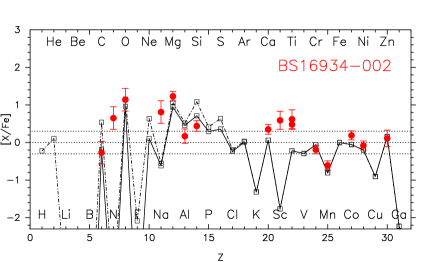
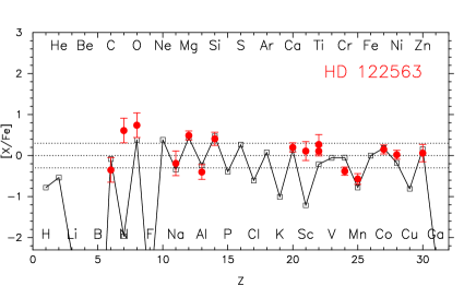
Figure 6: Comparison of the observed abundance patterns with predicted supernova yields. The upper panel shows the abundance pattern in BS 16934–002 compared with the predicted yield of 40 $M_{\odot}$, Population III supernova with explosion energy of 30 $\times 10^{51}$ ergs. The abundance patterns of the explosive yields, with and without undergoing significant mass ejection up to the CO-rich layer, are shown by the solid and dot-dashed lines, respectively. The lower panel shows a comparison of the abundance pattern observed in HD 122563 with that of predicted Population III supernova yields integrated over a Salpeter Initial Mass Function with a mass range of 11-50 $M_{\odot}$.

We have carried out a nucleosynthesis calculation for a supernova whose progenitor is a 40 $M_{\odot}$, zero-metallicity (Population III) star exploded with an explosion energy of $3\times 10^{52}$erg (a hypernova whose explosion energy is larger than $1\times 10^{52}$ erg, e.g., Umeda & Nomoto 2005; Tominaga et al. 2006a). The high explosion energy is adopted to explain the large enhancement of Co observed in BS 16934–002 (Umeda & Nomoto 2002). We assume the mixing-fallback model, where the explosively burned materials are mixed into the region of $M_{r}=$ 2.67–8.06 $M_{\odot}$, and only a fraction, $f=0.025$, of the mixed materials is ejected (the ejected Fe mass being 0.04 $M_{\odot}$), in order to approximately reproduce the overall abundance pattern of BS 16934–002 (dot-dashed line in the upper panel of Figure 6). Such large scale mixing and small amount of Fe ejection in the hypernova explosion can be realized in a jet-like explosion (Maeda & Nomoto 2003; Tominaga et al. 2007). In this model, the electron fraction, $Y_{e}$, in the explosive Si-burning layer is modified to $Y_{e}=$0.5001 and 0.4997 in the complete and incomplete Si-burning layers, respectively. This alteration of $Y_{e}$ in the inner region can be realized by the interaction of inner materials with neutrinos emitted from the collapsed remnant (Fröhlich et al. 2006; Iwamoto et al. 2006, in preparation). However, note that Figure  6 (dot-dashed line) shows that our calculation predicts a large overabundance of carbon, which is not observed for BS 16934–002.

The observed ratios of [C/O] $\sim-1.4$ and [C/Mg] $\sim-1.5$ in BS 16934–002 are extremely low among known extremely metal-poor stars. We find that both ratios are $-0.8$ or higher in our Population III supernova yields in the mass range 13-50 $M_{\odot}$. Carbon is mainly produced by triple-$\alpha$ reactions, and is located above the O and Mg-rich layers. Thus, one possible modification of the above model that might explain the lack of observed C-enhancement in BS 16934–002 is to consider the effects of significant mass loss from layers containing C-rich material from its massive progenitor during its evolution. This is an extension of the models of SN Ib and SN Ic, where the H and He envelopes, respectively, have been removed, possibly through transfer across a binary. Binary-modulated stripping is suggested for the SN IIb SN2001ig (Ryder et al. 2004, MNRAS, 349, 1093) and has been given additional credibility up by their subsequent discovery of a stellar-like object outliving the SN, which they believe to be the WR companion of the SN Ib/c (Ryder et al. 2006, MNRAS, 369, 32).

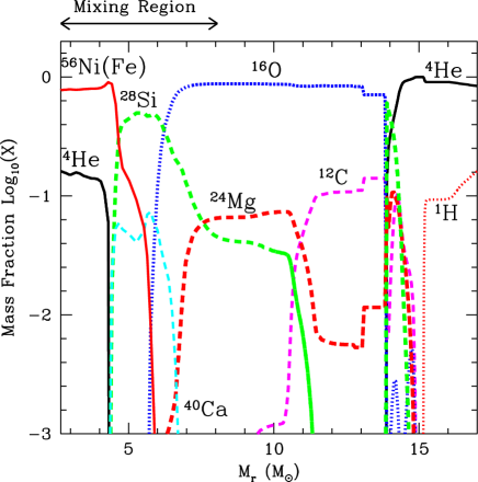
Figure 7: Internal abundance distribution of a 40 $M_{\odot}$, Population III hypernova model. Extensive mixing is assumed in the range $M_{r}=2.67$-8.06 $M_{\odot}$, and the ejection fraction from the mixing region is taken to be $f=0.025$. The ejecta have an Fe mass of 0.04 $M_{\odot}$. The region lost by an assumed significant mass ejection during the evolution of the massive progenitor is taken to be $M_{r}>11.65~{}M_{\odot}$.

We calculated the internal abundance distribution of the 40 $M_{\odot}$, Population III hypernova model, and show the results in Figure 7. The loss of H, He, and CO-rich outer layers could be explained by common-envelope evolution in a close binary system, and later by wind-mass loss during the He and CO star phases of the progenitor evolution. The solid line in the upper panel of Figure 6 shows the abundance pattern calculated assuming significant mass ejection prior to explosion. We note here that the ejection of He and C-rich layers may slightly affect the internal abundance distribution even if the H-envelope is lost during or after the core He burning phase. However, such effect is not included in the model calculation here. The observed abundance ratios of [C/Mg] and [C/Fe] in BS 16934–002 are reproduced by this model. Here, one important concern is that the C ejected before the explosion might be swept up by the shock wave, and then possibly mixed with the supernova ejecta. The mixing process between the circumstellar matter (CSM) and supernova ejecta is still uncertain, and we here assume that the mixing with the nearby CSM is inefficient.

The observed excesses of elements with odd atomic numbers (N, Na, and Sc) are not explained by the above models. The excess of N ([N/Fe] = +0.65) could be a result of internal processes (e.g., the first dredge-up) during the evolution of BS 16934–002 itself. Indeed, a similar overabundance of N is also found in HD 122563, which has similar atmospheric parameters, and is likely to be in a similar evolutionary stage. The underproduction of Sc in our supernova model is a problem in explaining the abundances of both BS 16934–002 and HD 122563 (see below for the latter object). This may be improved by using yields of nucleosynthesis in the explosion under low-density conditions (Umeda & Nomoto, 2005), and/or a neutrino-driven nucleosynthesis (Fröhlich et al., 2006). Neutrino-driven nucleosynthesis may also account for the overproduction of Ti isotopes observed in BS 16934–002 (Pruet et al., 2005; Fröhlich et al., 2006). The overabundance of Na in BS 16934–002 is possibly explained by overshooting in the convective C burning shell during the evolution of the massive-star progenitor, as suggested by Iwamoto et al. (2005). The Na abundance ejected by a supernova is determined by the extents of mixing and fallback regions. This is a possible reason for the fact that the Na overabundance is found in BS 16934–002 but is not seen in other objects.

Another important difference between BS 16934–002 and the two CEMP-$\alpha$ stars CS 22949–037 and CS 29498–043 might be their iron abundances. BS 16934–002 has a significantly higher iron abundance ([Fe/H] $=-2.8$) than the other two stars (both of which have [Fe/H] $\leq-3.5$). The EMP stars are considered to be formed from the ejecta of a single Population III or Population II supernova by supernova shock compression. The metallicities of EMP stars are determined by the ejected Fe mass, $M$(Fe), and the explosion energy $E$ ($E_{51}$: in units of $10^{51}$ ergs) of the parent supernova as follows (a supernova-induced star formation model, see Cioffi, McKee, & Bertschinger 1988; Ryan, Norris, & Beers 1996; Shigeyama & Tsujimoto 1998; Umeda & Nomoto 2005; Tominaga et al. 2006):

$${\rm[Fe/H]} = \log_{10}(M{\rm(Fe)}/M{\rm(H)})-\log_{10}{(X{\rm(Fe)}/X{\rm(H)})_{\odot}}$$ (1)

$$\simeq \log_{10}\left({M({\rm Fe})/{M_{\odot}}\over{E_{51}}}\right)-C.$$

where $M$(H) is the swept-up H mass, being roughly proportional to the explosion energy $E$, and $C$ is a “constant” value as a function of the density and sound speed of the CSM.

In the context of a supernova-induced star formation model, CS 29498–043 ([Fe/H]$=-3.75$, Aoki et al. 2004) can be reproduced with “constant” $C=0.8$ (a model with $M{\rm(Fe)}=0.0011M_{\odot}$ and $E_{51}=1$, as shown in Figure 9a of Umeda & Nomoto 2005). If the same constant $C$ is applied to BS 16934–002, the predicted [Fe/H] of BS 16934–002 would be [Fe/H]$=-3.7$, similar to CS 29498–043, because of the large explosion energy ($E_{51}=30$), in spite of the large amount of Fe ejection ($M{\rm(Fe)}=0.04M_{\odot}$). Therefore, BS 16934–002 might have been formed from the ejecta of a Population II supernova that already had a higher metallicity, e.g., [Fe/H]$\sim-3$. However, the star-formation process is affected by the uncertain distribution of the surrounding gas in the early Galaxy. Thus, there remains the possibility that Population III hypernovae form a portion of the [Fe/H] $\sim-3$ stars.

On the other hand, HD 122563 has a metallicity [Fe/H] $=-2.6$, thus is a likely second- or later-generation star (e.g., Tumlinson, 2006). Therefore, we model the abundance pattern of HD 122563 using the yields integrated over a mass range of 11-50 $M_{\odot}$ with a Salpeter Initial Mass Function, as shown in the lower panel of Figure 6. The Population III supernova models employed are ($M_{\rm MS}$, $E_{51}$) = (13,1), (15,1), (18,1), (20,10), (25,10), (30,20), (40,30), and (50,40) (Kobayashi et al. 2006; Nomoto et al. 2006; Tominaga et al. 2006), where $M_{\rm MS}$ is the main-sequence mass of the progenitor in solar masses. These models, with $M_{\rm MS}>20M_{\odot}$, are assumed to explode as hypernovae and undergo mixing-fallback. Small variations of $Y_{e}$ are assumed, as in the model for BS 16934–002 discussed above. We note that the yields of Population III supernovae can be used even if HD 122563 is actually formed from the ejecta of Population II supernovae, because the explosive yield of a Population III model is not so different from that of a model with [Fe/H] $=-3$ (Tominaga et al. 2006).

We have considered supernova explosions in an interacting binary system to explain the significant mass loss from the massive progenitor of BS 16934–002. Our interpretation, however, raises important questions as to why BS 16934–002 has such a peculiar composition, and why it alone BS 16934–002 might require binarity in order to explain the observed abundance pattern. More investigations are clearly necessary to resolve these questions.

4.3 The Spread of Mg/Fe in Extremely Metal-Poor Stars

The small spread of the observed abundance ratios of the $\alpha$ elements (e.g., [Mg/Fe]) in very metal-poor stars has been emphasized by recent work (e.g. Cayrel et al., 2004; Arnone et al., 2005). The bulk of halo stars exhibit moderate overabundances of Mg, with star-to-star scatter as small as 0.1 dex, while much larger scatter is found for other elements, such as the neutron-capture elements. One possible interpretation for the small spread of the [Mg/Fe] ratios is that the Galactic halo was well mixed even in the earliest phases of its evolution (François et al., 2004). The Mg abundance of BS 16934–002 clearly deviates from the trend found in halo stars, suggesting that this star has a rather different nucleosynthesis history than the majority of halo objects. Other stars that exhibit departures from the abundance trend of the $\alpha$ elements are the ADMP stars, with large underabundances of Mg (e.g. Ivans et al., 2003); these abundance patterns are not simply explained by any combination of the yields of Type Ia and II supernovae. Understanding the abundance patterns of AEMP stars, as well as those of ADMP stars, remains a challenge for studies of the nucleosynthesis processes that pertain to low-mass stars in the very early Galaxy.

Although recent studies based on high-resolution spectroscopy have revealed the chemical compositions of a significant number of EMP stars, much larger studies are required in order to better understand the observed abundance trends, and the scatter about these trends, in halo stars. In particular, for the lowest metallicity range ($-4.0\lesssim$ [Fe/H] $\lesssim-3.5$), at least two Mg-enhanced objects are known among the relatively small number of stars (10–20 objects) investigated do date, suggesting that a large scatter of the Mg abundance ratios may exist in this metallicity regime. The AEMP star BS 16934–002 might provide the first clues for developing an understanding of the relationship between the abundance scatter of $\alpha$ elements in the lowest metallicity range and the clear trend found at relatively higher metallicity.

Table 1: PROGRAM STARS AND OBSERVATIONS

Star	Wavelength	Exp.	S/N	Obs. date (JD)	Radial velocity
	( Å)	(minutes)			(km s-1)
BS 16934–002	4030–6800	60 (2)	100/1	31 May, 2004 (2453158)	$82.5\pm 0.3$
HD 122563	4030–6800	2 (2)	300/1	19 June, 2005 (2453541)	$-26.0\pm 0.2$

Table 2: EQUIVALENT WIDTHS

Species	wavelength	$\log gf$	L.E.P.	HD 122563	BS 16934–002	Remarks
O I	6300.300	-9.820	0.000	7.2	14.3
O I	6363.776	-10.303	0.020	2.2	5.0
Na I	5682.633	-0.700	2.102	1.3	8.7
Na I	5688.204	-0.412	2.104	2.8	17.7
Na I	5889.951	0.101	0.000	…	225.6
Na I	5895.924	-0.197	0.000	…	212.0
Mg I	3829.355	-0.210	2.709	182.1	…
Mg I	3986.753	-1.030	4.346	35.4	…
Mg I	4057.505	-0.890	4.346	…	72.8
Mg I	4167.271	-0.770	4.346	54.4	84.6
Mg I	4571.096	-5.688	0.000	84.8	113.3
Mg I	4702.991	-0.520	4.346	73.8	106.8
Mg I	5172.685	-0.380	2.712	201.7	…
Mg I	5183.604	-0.160	2.717	221.8	…
Mg I	5528.404	-0.490	4.346	77.6	112.9
Mg I	5711.088	-1.720	4.346	11.7	31.7
Al I	3944.006	-0.644	0.000	163.0	…
Al I	3961.520	-0.340	0.014	139.0	153.3
Si I	3905.523	-0.980	1.909	196.6	…
Si I	4102.936	-2.910	1.909	88.8	78.5
Ca I	4226.728	0.244	0.000	…	201.5
Ca I	4283.010	-0.220	1.886	62.7	68.3
Ca I	4318.652	-0.210	1.899	53.7	52.7
Ca I	4425.441	-0.360	1.879	49.1	45.9
Ca I	4435.688	-0.520	1.886	41.5	38.2
Ca I	4454.781	0.260	1.899	…	83.3
Ca I	4455.887	-0.530	1.899	39.8	43.9
Ca I	5262.244	-0.471	2.521	34.2	44.6
Ca I	5581.971	-0.555	2.523	13.1	12.0
Ca I	5588.757	0.358	2.526	49.6	49.4
Ca I	5590.120	-0.571	2.521	12.3	12.0
Ca I	5594.468	0.097	2.523	36.7	36.2
Ca I	5598.487	-0.087	2.521	29.9	28.6
Ca I	5601.285	-0.523	2.526	13.1	10.7
Ca I	5857.452	0.240	2.933	24.3	25.5
Ca I	6102.722	-0.770	1.879	36.8	39.4
Ca I	6122.219	-0.320	1.886	68.5	64.4
Ca I	6169.055	-0.797	2.523	9.4	10.3
Ca I	6169.559	-0.478	2.526	16.3	14.5
Ca I	6439.073	0.390	2.526	58.8	61.4
Ca I	6449.810	-0.502	2.521	16.5	16.0
Ca I	6499.649	-0.818	2.523	9.4	10.7
Ca I	6717.685	-0.524	2.709	11.1	13.0
Sc I	4995.002	-0.880	2.111	1.0	…
Ti I	3904.784	0.030	0.900	29.6	35.3
Ti I	3924.526	-0.881	0.021	35.1	48.0
Ti I	3989.759	-0.142	0.021	71.7	86.5
Ti I	3998.637	0.000	0.048	71.5	84.2
Ti I	4008.928	-1.016	0.021	29.5	41.4
Ti I	4512.733	-0.424	0.836	14.1	27.4
Ti I	4533.239	0.532	0.848	52.9	67.4
Ti I	4534.775	0.336	0.836	42.2	57.2
Ti I	4535.567	0.120	0.826	36.2	50.1
Ti I	4544.687	-0.520	0.818	14.9	22.3
Ti I	4548.763	-0.298	0.826	17.9	28.0
Ti I	4681.908	-1.015	0.048	29.5	48.2
Ti I	4981.730	0.560	0.848	62.2	…
Ti I	4991.066	0.436	0.836	58.1	73.2
Ti I	4999.501	0.306	0.826	50.2	66.6
Ti I	5007.206	0.168	0.818	52.2	64.0
Ti I	5009.645	-2.203	0.021	…	5.7
Ti I	5016.160	-0.516	0.848	12.7	23.7
Ti I	5020.024	-0.358	0.836	18.3	30.1
Ti I	5024.843	-0.546	0.818	13.6	21.5
Ti I	5035.902	0.260	1.460	16.4	26.3
Ti I	5036.463	0.186	1.443	11.2	19.9
Ti I	5038.396	0.069	1.430	…	18.7
Ti I	5039.960	-1.130	0.020	29.9	51.0
Ti I	5064.651	-0.935	0.048	35.4	53.1
Ti I	5173.740	-1.062	0.000	33.4	50.3
Ti I	5192.969	-0.948	0.021	38.3	55.1
Ti I	5210.384	-0.828	0.048	42.6	62.6
Ti I	6258.099	-0.299	1.443	5.4	8.6
V I	4379.230	0.550	0.301	30.6	48.6
V I	4786.499	0.110	2.074	16.0	9.8
V I	5195.395	-0.120	2.278	11.8	7.2
V I	6008.648	-2.340	1.183	6.1	4.0
Cr I	3908.762	-1.000	1.004	21.6	…
Cr I	4254.332	-0.114	0.000	113.1	118.6
Cr I	4274.796	-0.231	0.000	112.9	109.3
Cr I	4337.566	-1.112	0.968	19.3	26.4
Cr I	4558.650	-0.660	4.070	19.0	21.8
Cr I	4580.056	-1.650	0.941	16.7	16.2
Cr I	4588.200	-0.630	4.070	12.7	15.0
Cr I	4600.752	-1.260	1.004	16.6	19.4
Cr I	4616.137	-1.190	0.983	19.9	22.1
Cr I	4626.188	-1.320	0.968	16.8	15.6
Cr I	4646.174	-0.700	1.030	35.6	…
Cr I	4651.285	-1.460	0.983	11.8	13.4
Cr I	4652.158	-1.030	1.004	24.6	29.3
Cr I	5206.039	0.019	0.941	85.8	91.3
Cr I	5247.564	-1.640	0.961	9.8	13.6
Mn I	3823.508	0.058	2.143	16.6	…
Mn I	4030.753	-0.470	0.000	138.4	122.9
Mn I	4033.062	-0.618	0.000	125.6	116.6
Mn I	4034.483	-0.811	0.000	117.4	112.3
Mn I	4041.357	0.285	2.114	45.3	27.4
Mn I	4754.048	-0.086	2.282	19.2	13.9
Mn I	4783.432	0.042	2.298	23.6	16.1
Mn I	4823.528	0.144	2.319	25.9	16.1
Fe I	3787.880	-0.859	1.011	144.9	134.0
Fe I	3805.342	0.310	3.301	66.2	54.8
Fe I	3815.840	0.226	1.485	174.2	161.7
Fe I	3827.823	0.062	1.557	159.9	152.4
Fe I	3839.256	-0.330	3.047	50.4	55.0
Fe I	3840.437	-0.506	0.990	165.4	146.4
Fe I	3841.048	-0.065	1.608	144.1	134.3
Fe I	3845.169	-1.390	2.424	44.7	35.6
Fe I	3846.800	-0.020	3.251	55.0	51.0
Fe I	3849.980	-0.863	1.010	149.5	131.7
Fe I	3850.818	-1.745	0.990	…	117.6
Fe I	3852.573	-1.180	2.176	71.5	63.6
Fe I	3856.372	-1.286	0.052	182.2	178.9
Fe I	3863.741	-1.430	2.692	39.8	31.4
Fe I	3865.523	-0.982	1.011	149.0	141.0
Fe I	3867.216	-0.450	3.017	46.7	41.6
Fe I	3885.510	-1.090	2.424	58.6	42.5
Fe I	3899.707	-1.531	0.087	172.1	156.8
Fe I	3902.946	-0.466	1.557	136.8	118.9
Fe I	3917.181	-2.155	0.990	108.4	…
Fe I	3920.258	-1.746	0.121	161.9	156.0
Fe I	3922.912	-1.651	0.052	172.7	163.6
Fe I	3940.878	-2.600	0.958	83.5	84.1
Fe I	3949.953	-1.250	2.176	67.1	73.5
Fe I	3977.741	-1.120	2.198	74.8	71.5
Fe I	4001.661	-1.900	2.176	37.7	…
Fe I	4005.242	-0.610	1.557	132.2	119.5
Fe I	4007.272	-1.280	2.759	28.6	31.3
Fe I	4014.531	-0.590	3.047	71.8	…
Fe I	4021.866	-0.730	2.759	54.2	…
Fe I	4032.627	-2.380	1.485	54.0	45.3
Fe I	4044.609	-1.220	2.832	32.3	…
Fe I	4058.217	-1.110	3.211	30.7	26.4
Fe I	4062.441	-0.860	2.845	45.7	43.9
Fe I	4063.594	0.060	1.557	166.0	151.8
Fe I	4067.271	-1.419	2.559	41.4	32.5
Fe I	4067.978	-0.470	3.211	43.4	35.3
Fe I	4070.769	-0.790	3.241	27.1	22.4
Fe I	4071.738	-0.022	1.608	156.2	144.1
Fe I	4073.763	-0.900	3.266	22.2	…
Fe I	4079.838	-1.360	2.858	22.7	18.7
Fe I	4095.970	-1.480	2.588	…	27.4
Fe I	4098.176	-0.880	3.241	25.5	…
Fe I	4109.057	-1.560	3.292	11.7	15.3
Fe I	4109.802	-0.940	2.845	45.0	44.9
Fe I	4114.445	-1.300	2.832	30.1	26.5
Fe I	4120.207	-1.270	2.990	24.3	16.7
Fe I	4121.802	-1.450	2.832	24.4	20.9
Fe I	4132.899	-1.010	2.845	43.3	38.9
Fe I	4136.998	-0.450	3.415	26.7	25.1
Fe I	4139.927	-3.629	0.990	…	28.9
Fe I	4143.414	-0.200	3.047	67.1	58.4
Fe I	4143.868	-0.510	1.557	135.2	123.9
Fe I	4147.669	-2.104	1.485	80.4	74.2
Fe I	4152.169	-3.232	0.958	60.8	49.9
Fe I	4153.899	-0.320	3.397	40.7	32.8
Fe I	4154.499	-0.690	2.832	54.0	43.7
Fe I	4154.805	-0.400	3.368	39.8	32.9
Fe I	4156.799	-0.810	2.832	59.3	51.6
Fe I	4157.779	-0.400	3.417	37.3	38.0
Fe I	4158.793	-0.670	3.430	22.4	17.4
Fe I	4175.636	-0.830	2.845	52.1	47.5
Fe I	4181.755	-0.370	2.832	75.4	68.8
Fe I	4182.382	-1.180	3.017	24.5	16.6
Fe I	4184.892	-0.870	2.832	45.2	39.4
Fe I	4187.039	-0.548	2.450	89.5	80.7
Fe I	4191.430	-0.670	2.469	84.9	…
Fe I	4195.329	-0.490	3.332	44.2	39.0
Fe I	4196.208	-0.700	3.397	23.1	19.8
Fe I	4199.095	0.160	3.047	80.0	75.6
Fe I	4216.184	-3.356	0.000	115.3	108.5
Fe I	4222.213	-0.967	2.450	…	69.8
Fe I	4227.426	0.270	3.332	91.9	…
Fe I	4233.603	-0.604	2.482	85.3	80.6
Fe I	4238.810	-0.230	3.397	44.2	39.8
Fe I	4247.426	-0.240	3.368	50.6	44.6
Fe I	4250.119	-0.405	2.469	94.4	81.0
Fe I	4250.787	-0.710	1.557	129.1	…
Fe I	4260.474	0.080	2.399	119.4	111.7
Fe I	4271.153	-0.349	2.450	103.8	96.4
Fe I	4271.761	-0.164	1.485	163.7	152.4
Fe I	4282.403	-0.780	2.176	92.1	84.4
Fe I	4325.762	0.010	1.608	162.0	150.4
Fe I	4337.046	-1.695	1.557	94.5	…
Fe I	4352.735	-1.290	2.223	77.7	72.1
Fe I	4375.930	-3.031	0.000	124.8	122.2
Fe I	4407.709	-1.970	2.176	59.0	…
Fe I	4422.568	-1.110	2.845	45.6	…
Fe I	4430.614	-1.659	2.223	54.6	46.2
Fe I	4442.339	-1.255	2.198	78.7	75.3
Fe I	4443.194	-1.040	2.858	38.1	31.7
Fe I	4447.717	-1.342	2.223	73.8	65.1
Fe I	4454.381	-1.300	2.832	…	29.6
Fe I	4459.118	-1.279	2.176	92.3	76.4
Fe I	4461.653	-3.210	0.087	119.0	112.4
Fe I	4466.552	-0.600	2.832	86.3	77.0
Fe I	4476.019	-0.820	2.845	67.6	57.3
Fe I	4484.220	-0.860	3.603	17.2	16.6
Fe I	4489.739	-3.966	0.121	87.4	80.6
Fe I	4490.083	-1.580	3.017	9.6	6.6
Fe I	4494.563	-1.136	2.198	84.6	77.9
Fe I	4528.614	-0.822	2.176	102.8	96.4
Fe I	4531.148	-2.155	1.485	84.9	74.8
Fe I	4592.651	-2.449	1.557	68.3	63.0
Fe I	4602.941	-2.210	1.485	82.5	78.1
Fe I	4611.185	-2.720	2.851	15.3	…
Fe I	4632.912	-2.913	1.608	34.4	28.0
Fe I	4647.435	-1.350	2.949	24.3	21.1
Fe I	4678.846	-0.830	3.603	17.9	16.4
Fe I	4691.411	-1.520	2.990	20.1	20.5
Fe I	4707.274	-1.080	3.241	28.5	…
Fe I	4710.283	-1.610	3.018	15.6	14.8
Fe I	4733.591	-2.990	1.485	40.3	35.3
Fe I	4736.772	-0.750	3.211	44.1	36.0
Fe I	4786.807	-1.610	3.017	15.6	…
Fe I	4789.650	-0.960	3.547	12.1	8.7
Fe I	4859.741	-0.760	2.876	…	53.2
Fe I	4871.318	-0.360	2.865	79.4	73.2
Fe I	4872.138	-0.570	2.882	68.1	59.7
Fe I	4890.755	-0.390	2.876	80.2	70.6
Fe I	4891.492	-0.110	2.851	93.5	84.7
Fe I	4903.310	-0.930	2.882	50.7	45.3
Fe I	4918.994	-0.340	2.865	81.4	75.8
Fe I	4920.502	0.070	2.833	104.1	96.6
Fe I	4924.770	-2.256	2.279	30.3	22.6
Fe I	4938.814	-1.080	2.876	42.3	35.0
Fe I	4939.687	-3.340	0.859	71.1	61.9
Fe I	4946.388	-1.170	3.368	15.9	…
Fe I	4966.088	-0.870	3.332	31.3	26.6
Fe I	4973.102	-0.950	3.960	8.8	…
Fe I	4994.130	-2.956	0.915	82.2	74.5
Fe I	5001.870	0.050	3.880	31.6	25.0
Fe I	5006.119	-0.610	2.833	71.6	66.2
Fe I	5012.068	-2.642	0.859	110.5	105.3
Fe I	5014.942	-0.300	3.943	23.3	18.0
Fe I	5022.236	-0.530	3.984	13.8	12.6
Fe I	5027.225	-1.890	3.640	9.9	…
Fe I	5028.127	-1.120	3.573	9.5	4.2
Fe I	5041.072	-3.090	0.958	86.1	81.0
Fe I	5041.756	-2.200	1.485	94.3	87.3
Fe I	5044.210	-2.040	2.850	9.6	…
Fe I	5049.820	-1.344	2.279	74.4	66.5
Fe I	5051.635	-2.795	0.915	100.5	92.5
Fe I	5060.080	-5.460	0.000	19.4	16.2
Fe I	5068.766	-1.040	2.940	39.7	31.8
Fe I	5074.749	-0.200	4.220	17.5	14.7
Fe I	5079.224	-2.067	2.198	43.3	36.9
Fe I	5079.740	-3.220	0.990	70.0	…
Fe I	5080.950	-3.090	3.267	17.1	…
Fe I	5083.339	-2.958	0.958	86.6	79.3
Fe I	5090.770	-0.360	4.260	7.1	4.8
Fe I	5098.697	-2.030	2.176	54.7	47.8
Fe I	5123.720	-3.068	1.011	76.8	…
Fe I	5125.117	-0.140	4.220	17.5	14.0
Fe I	5127.359	-3.307	0.915	70.4	65.8
Fe I	5131.468	-2.510	2.223	20.6	16.2
Fe I	5133.689	0.140	4.178	31.0	26.8
Fe I	5137.382	-0.400	4.178	14.4	11.5
Fe I	5141.739	-1.964	2.424	19.3	18.1
Fe I	5142.929	-3.080	0.958	82.5	73.1
Fe I	5150.839	-3.003	0.990	73.4	61.6
Fe I	5151.911	-3.322	1.011	61.7	54.0
Fe I	5162.273	0.020	4.178	26.2	19.5
Fe I	5166.282	-4.195	0.000	92.2	85.4
Fe I	5171.597	-1.793	1.485	108.3	104.3
Fe I	5191.455	-0.550	3.038	60.4	51.0
Fe I	5192.344	-0.420	2.998	69.8	61.4
Fe I	5194.942	-2.090	1.557	89.9	85.2
Fe I	5198.711	-2.135	2.223	37.1	31.4
Fe I	5202.336	-1.838	2.176	59.2	48.8
Fe I	5204.583	-4.332	0.087	128.3	…
Fe I	5216.274	-2.150	1.608	82.8	78.5
Fe I	5217.390	-1.070	3.211	22.7	19.7
Fe I	5225.525	-4.789	0.110	44.8	39.1
Fe I	5232.940	-0.060	2.940	92.2	85.3
Fe I	5242.491	-0.970	3.634	11.7	9.9
Fe I	5247.050	-4.946	0.087	36.7	33.2
Fe I	5250.210	-4.938	0.121	35.4	28.5
Fe I	5250.646	-2.180	2.198	40.9	33.2
Fe I	5254.956	-4.764	0.110	…	42.2
Fe I	5263.305	-0.879	3.266	27.8	19.9
Fe I	5269.537	-1.321	0.859	165.8	156.2
Fe I	5281.790	-0.830	3.038	44.8	42.3
Fe I	5283.621	-0.432	3.241	52.1	45.9
Fe I	5302.300	-0.720	3.283	…	28.2
Fe I	5307.361	-2.987	1.608	33.7	28.8
Fe I	5324.179	-0.103	3.211	72.4	65.0
Fe I	5328.039	-1.466	0.915	159.7	149.9
Fe I	5328.531	-1.850	1.557	107.1	96.6
Fe I	5332.900	-2.780	1.557	44.6	38.5
Fe I	5501.465	-3.050	0.958	87.7	79.9
Fe I	5506.778	-2.797	0.990	99.8	91.4
Fe I	5569.618	-0.540	3.417	37.5	31.1
Fe I	5572.842	-0.275	3.397	50.8	44.6
Fe I	5576.088	-1.000	3.430	22.4	18.3
Fe I	5586.755	-0.096	3.368	61.3	57.8
Fe I	5615.644	0.050	3.332	72.2	67.6
Fe I	5624.542	-0.755	3.417	26.9	22.5
Fe I	5658.816	-0.793	3.397	26.8	22.6
Fe I	5686.529	-0.450	4.549	3.0	…
Fe I	5701.543	-2.216	2.559	14.8	12.2
Fe I	6065.481	-1.530	2.609	43.3	39.4
Fe I	6136.614	-1.400	2.453	66.1	58.3
Fe I	6137.691	-1.403	2.588	56.5	48.4
Fe I	6191.558	-1.420	2.433	64.0	56.9
Fe I	6200.312	-2.437	2.609	9.4	8.1
Fe I	6213.429	-2.480	2.223	20.7	16.7
Fe I	6219.280	-2.433	2.198	26.8	23.6
Fe I	6230.723	-1.281	2.559	67.9	60.8
Fe I	6246.318	-0.733	3.603	…	16.0
Fe I	6252.555	-1.687	2.404	53.8	48.6
Fe I	6254.257	-2.443	2.279	24.4	21.7
Fe I	6265.134	-2.550	2.176	24.9	20.1
Fe I	6301.499	-0.718	3.654	17.5	14.2
Fe I	6322.685	-2.426	2.588	11.2	7.8
Fe I	6335.330	-2.180	2.198	37.7	34.9
Fe I	6336.835	-1.050	3.686	12.9	10.5
Fe I	6393.601	-1.432	2.433	61.0	53.2
Fe I	6400.000	-0.290	3.603	39.5	33.6
Fe I	6411.649	-0.595	3.654	23.1	20.0
Fe I	6421.350	-2.027	2.279	46.3	39.6
Fe I	6430.845	-2.006	2.176	55.6	50.2
Fe I	6498.940	-4.699	0.958	9.7	…
Fe I	6592.913	-1.470	2.728	…	33.2
Fe I	6593.868	-2.422	2.433	15.9	13.7
Fe I	6663.440	-2.479	2.424	15.9	12.9
Fe I	6677.986	-1.420	2.692	50.7	44.5
Fe I	6750.151	-2.621	2.424	12.2	14.0
Co I	3842.047	-0.770	0.923	56.7	54.7
Co I	3845.468	0.010	0.923	93.6	86.9
Co I	3873.120	-0.660	0.432	129.9	121.4
Co I	3881.869	-1.130	0.582	78.0	75.8
Co I	3995.306	-0.220	0.923	82.7	…
Co I	4020.898	-2.070	0.432	40.6	34.2
Co I	4110.532	-1.080	1.049	39.0	31.7
Co I	4121.318	-0.320	0.923	91.4	88.6
Ni I	3807.144	-1.220	0.423	115.4	107.4
Ni I	3858.301	-0.951	0.423	126.6	114.3
Ni I	4648.659	-0.160	3.420	16.2	11.2
Ni I	4714.421	0.230	3.380	31.6	22.8
Ni I	4855.414	0.000	3.542	…	10.0
Ni I	4980.161	-0.110	3.606	15.6	10.3
Ni I	5017.591	-0.080	3.539	14.5	8.3
Ni I	5035.374	0.290	3.635	21.7	16.4
Ni I	5080.523	0.130	3.655	21.8	17.1
Ni I	5084.081	0.030	3.678	12.4	7.3
Ni I	5137.075	-1.990	1.676	35.5	26.1
Ni I	5578.734	-2.640	1.676	6.4	4.1
Ni I	5754.675	-2.330	1.935	11.8	9.6
Ni I	6108.121	-2.450	1.676	10.9	7.3
Ni I	6643.641	-2.300	1.676	25.1	19.6
Ni I	6767.778	-2.170	1.826	23.4	14.5
Zn I	4722.150	-0.390	4.030	14.2	11.1
Zn II	4810.530	-0.170	4.080	18.8	16.4
Sc II	4246.820	0.240	0.315	133.0	152.4
Sc II	4324.998	-0.440	0.595	96.7	109.7
Sc II	4415.544	-0.670	0.595	74.2	89.6
Sc II	5031.010	-0.400	1.357	41.9	63.9
Sc II	5239.811	-0.770	1.455	20.3	34.3
Sc II	5318.374	-2.010	1.357	2.9	6.3
Sc II	5526.785	0.020	1.768	41.4	63.8
Sc II	5641.000	-1.130	1.500	13.3	26.4
Sc II	5657.907	-0.600	1.507	32.1	52.0
Sc II	5658.362	-1.210	1.497	10.6	21.1
Sc II	5667.164	-1.310	1.500	8.3	19.3
Sc II	5669.055	-1.200	1.500	10.1	21.4
Sc II	5684.214	-1.070	1.507	11.8	25.6
Sc II	6604.578	-1.310	1.357	8.7	20.9
Ti II	3813.394	-2.020	0.607	97.0	…
Ti II	3882.291	-1.710	1.116	…	79.3
Ti II	4012.396	-1.750	0.574	104.8	113.5
Ti II	4025.120	-1.980	0.607	86.1	93.7
Ti II	4028.355	-1.000	1.892	55.4	68.7
Ti II	4053.829	-1.210	1.893	42.6	52.7
Ti II	4161.527	-2.160	1.084	53.3	63.1
Ti II	4163.634	-0.400	2.590	45.0	55.6
Ti II	4184.309	-2.510	1.080	30.7	42.8
Ti II	4330.723	-2.060	1.180	46.9	63.1
Ti II	4337.876	-1.130	1.080	101.4	112.9
Ti II	4395.833	-1.970	1.243	49.4	57.5
Ti II	4399.786	-1.270	1.237	97.1	102.2
Ti II	4417.715	-1.430	1.165	99.6	107.2
Ti II	4418.306	-1.990	1.237	53.2	60.0
Ti II	4441.731	-2.410	1.180	39.7	56.0
Ti II	4443.775	-0.700	1.080	119.9	128.3
Ti II	4444.536	-2.210	1.116	48.1	60.7
Ti II	4450.503	-1.510	1.084	88.5	92.1
Ti II	4464.461	-2.080	1.161	68.0	79.3
Ti II	4468.517	-0.600	1.131	121.7	132.5
Ti II	4470.835	-2.280	1.165	48.3	59.7
Ti II	4488.342	-0.820	3.124	7.7	16.1
Ti II	4501.269	-0.760	1.116	117.4	121.1
Ti II	4529.480	-2.030	1.572	44.0	56.7
Ti II	4533.972	-0.770	1.237	122.3	130.9
Ti II	4545.144	-1.810	1.131	32.3	44.8
Ti II	4563.770	-0.960	1.221	109.9	121.0
Ti II	4571.957	-0.530	1.572	110.8	123.6
Ti II	4583.408	-2.870	1.165	17.7	23.9
Ti II	4589.915	-1.790	1.237	73.9	86.2
Ti II	4657.212	-2.320	1.243	37.3	49.6
Ti II	4708.651	-2.370	1.237	33.8	47.7
Ti II	4779.979	-1.370	2.048	32.4	44.0
Ti II	4798.507	-2.670	1.080	31.9	43.7
Ti II	4805.089	-1.100	2.061	46.2	56.7
Ti II	4865.610	-2.810	1.116	25.6	35.1
Ti II	4911.175	-0.340	3.124	8.1	14.0
Ti II	5005.159	-2.730	1.566	7.9	12.6
Ti II	5129.155	-1.390	1.892	43.9	57.1
Ti II	5185.902	-1.350	1.893	36.7	50.3
Ti II	5188.691	-1.210	1.582	91.1	100.1
Ti II	5268.607	-1.620	2.598	3.8	9.4
Ti II	5336.778	-1.630	1.582	53.2	64.5
V II	3916.411	-1.053	1.428	34.6	45.6
V II	3951.960	-0.784	1.476	40.8	47.7
V II	4005.710	-0.522	1.820	32.4	42.4
V II	4023.378	-0.689	1.805	32.1	45.3
V II	4035.622	-0.767	1.793	48.9	52.4
Fe II	4178.855	-2.480	2.583	56.7	47.2
Fe II	4233.167	-2.000	2.583	…	77.2
Fe II	4416.817	-2.600	2.778	46.6	34.7
Fe II	4489.185	-2.970	2.828	24.1	21.8
Fe II	4491.401	-2.700	2.856	33.1	25.1
Fe II	4508.283	-2.580	2.856	51.5	43.6
Fe II	4515.337	-2.480	2.844	45.0	35.7
Fe II	4541.523	-3.050	2.856	22.0	15.5
Fe II	4555.890	-2.290	2.828	54.1	43.8
Fe II	4576.331	-2.940	2.844	22.1	18.2
Fe II	4583.829	-2.020	2.807	83.4	72.7
Fe II	4731.439	-3.360	2.891	17.7	10.2
Fe II	4923.930	-1.320	2.891	104.7	93.2
Fe II	4993.350	-3.670	2.810	7.3	…
Fe II	5018.450	-1.220	2.891	115.1	106.6
Fe II	5197.559	-2.100	3.230	38.7	30.1
Fe II	5234.619	-2.270	3.221	43.6	33.7
Fe II	5275.999	-1.940	3.199	50.8	40.2
Fe II	5284.080	-3.190	2.891	17.1	13.9
Fe II	5534.834	-2.930	3.245	15.4	12.9
Fe II	6247.545	-2.510	3.892	8.6	4.7
Sr II	4077.714	0.150	0.000	162.6	106.4
Sr II	4215.524	-0.180	0.000	151.1	95.3
Ba II	4554.033	0.163	0.000	100.3	58.0
Ba II	4934.086	-0.160	0.000	91.4	51.2
Ba II	6496.896	-0.369	0.604	…	12.1

Table 3: ATMOSPHERIC PARAMETERS

Star	$T_{\rm eff}$	$\log g$	[Fe/H]	$v_{\rm micro}$
BS 16934–002	4500	1.0	$-2.8$	2.1
HD 122563	4600	1.1	$-2.6$	2.2

Table 4: ABUNDANCE RESULTS

Element	Species	Solar Abundance	BS 16934–002					HD 122563
		$\log\epsilon$	$\log\epsilon$	[X/Fe]	$N$	$\sigma$		$\log\epsilon$	[X/Fe]	$N$	$\sigma$
C	CH	8.39	5.35	$-$0.27	$\cdots$	0.17		5.45	$-$0.35	$\cdots$	0.17
N	CN	7.78	5.65	+0.65	$\cdots$	0.29		5.80	+0.61	$\cdots$	0.29
O	O I	8.66	7.03	+1.14	2	0.19		6.81	+0.74	2	0.19
Na	Na I	6.17	4.20	+0.81	2	0.13		3.39	$-$0.19	2	0.13
Mg	Mg I	7.53	5.98	+1.23	6	0.13		5.44	+0.49	6	0.11
Al	Al I	6.37	3.76	+0.17	1	0.19		3.38	$-$0.40	1	0.18
Si	Si I	7.51	5.17	+0.44	4	0.14		5.34	+0.41	4	0.16
Ca	Ca I	6.31	3.89	+0.35	22	0.13		3.93	+0.20	20	0.11
Sc	Sc II	3.05	0.87	+0.59	14	0.24		0.57	+0.11	14	0.23
Ti	Ti I	4.90	2.61	+0.48	28	0.13		2.42	+0.11	27	0.12
Ti	Ti II	4.90	2.74	+0.62	42	0.25		2.58	+0.27	41	0.24
Cr	Cr I	5.64	2.67	$-$0.19	11	0.11		2.57	$-$0.38	13	0.10
Mn	Mn I	5.39	2.01	$-$0.61	6	0.12		2.23	$-$0.57	8	0.13
Fe	Fe I	7.45	4.68	$-$2.78	130	0.20		4.86	$-$2.59	214	0.20
Fe	Fe II	7.45	4.67	$-$2.79	20	0.19		4.87	$-$2.58	20	0.19
Co	Co I	4.92	2.34	+0.19	6	0.12		2.48	+0.15	7	0.11
Ni	Ni I	6.23	3.38	$-$0.08	16	0.12		3.66	+0.02	15	0.11
Zn	Zn I	4.60	1.94	+0.11	2	0.22		2.08	+0.06	2	0.21
Sr	Sr II	2.92	$-$1.22	$-$1.36	2	0.25		0.08	$-$0.30	2	0.15
Ba	Ba II	2.17	$-$2.29	$-$1.69	2	0.24		$-$1.69	$-$1.28	2	0.23

Figure 1: Comparison of the equivalent widths measured by Aoki et al. (2005) with those in the present work. The solid line indicates the result of a least-square fit, while the dotted line shows a line with a slope of unity.

Figure 2: Comparison of synthetic spectra for the CH band in BS 16934–002 with the observed one. The assumed abundances are [C/Fe]$=-0.27\pm 0.20$.

Figure 3: Same as Fig. 2, but for the CN band. The assumed abundances are [N/Fe]$=0.65\pm 0.30$.

Figure 4: Same as Fig. 2, but for the [O I] 6300 Å line for BS 16934–002 (upper panel) and HD 122563 (lower panel). The assumed abundances are [O/Fe]$=+1.14\pm 0.20$, and $+0.74\pm 0.20$ for BS 16934–002 and HD 122563, respectively. The positions of telluric lines, which are corrected using spectra of standard stars, are shown by the arrows.

Figure 5: Logarithmic abundance differences between BS 16934–002 and HD 122563 as a function of atomic number.

References

- (1)
- Aoki et al. (2005) Aoki, W., Honda, S., Beers, T. C., Kajino, T., Ando, H., Norris, J. E., Ryan, S. G., Izumiura, H., Sadakane, K., & Takada-Hidai, M. 2005, ApJ, 632, 611
- Aoki et al. (2002) Aoki, W., Norris, J. E., Ryan, S. G., Beers, T. C., & Ando, H. 2002, ApJ, 576, L141
- Aoki et al. (2004) Aoki, W., Norris, J. E., Ryan, S. G., Beers, T. C., Christlieb, N., Tsangarides, S., & Ando, H. 2004, ApJ, 608, 971
- Arlandini et al. (1999) Arlandini, C., Käppeler, F., Wisshak, K., Gallino, R., Lugaro, M., Busso, M., & Straniero, O. 1999, ApJ, 525, 886
- Arnone et al. (2005) Arnone, E., Ryan, S. G., Argast, D., Norris, J. E., & Beers, T. C. 2005, A&A, 430, 507
- Asplund et al. (2005) Asplund, M., Grevesse, N., & Sauval, A. J. 2005, ASP Conf. Ser. 336: Cosmic Abundances as Records of Stellar Evolution and Nucleosynthesis, 336, 25
- Asplund et al. (2004) Asplund, M., Grevesse, N., Sauval, A. J., Allende Prieto, C., & Kiselman, D. 2004, A&A, 417, 751
- Barbuy et al. (2003) Barbuy, B., Meléndez, J., Spite, M., Spite, F., Depagne, E., Hill, V., Cayrel, R., Bonifacio, P., Damineli, A., & Torres, C. A. O. 2003, ApJ, 588, 1072
- Beers & Christlieb (2005) Beers, T. C., & Christlieb, N. 2005, ARAA, 43, 531
- Cayrel et al. (2004) Cayrel, R., Depagne, E., Spite, M., Hill, V., Spite, F., Francois, P., Beers, T., Primas, F., Andersen, J., Barbuy, B., Bonifacio, P., Molaro, P., & Nordström, B. 2004, A&A, 416, 1117
- Cioffi, McKee, & Bertschinger (1988) Cioffi, D. F., McKee, C. F., Bertschinger, E. 1988, ApJ, 334, 252
- Depagne et al. (2002) Depagne, E., Hill, V., Spite, M., Spite, F., Plez, B., Beers, T., Barbuy, B., Cayrel, R., Andersen, J., Bonifacio, P., François, P., Nordström, B., & Primas, F. 2002, A&A, 390, 187
- François et al. (2004) François, P., Matteucci, F., Cayrel, R., Spite, M., Spite, F., & Chiappini, C. 2004, A&A, 421, 613
- Fröhlich et al. (2006) Fröhlich, C., et al. 2006, ApJ, 637, 415
- Honda et al. (2006) Honda, S., Aoki, W., Wanajo, S., Ishimaru, Y., & Ryan, S. G. 2006, ApJ, 643, 1180
- Ivans et al. (2003) Ivans, I. I., Sneden, C., James, C. R., Preston, G. W., Fulbright, J. P., Höflich, P. A., Carney, B. W., & Wheeler, J. C. 2003, ApJ, 592, 906
- Iwamoto et al. (2005) Iwamoto, N., Umeda, H., Tominaga, N., Nomoto, K., & Maeda, K. 2005, Science, 309, 451
- Kobayashi et al. (2006) Kobayashi, C., Umeda, H., Nomoto, K., Tominaga, N., & Ohkubo, T. 2006, ApJ, in press (astroph/0608688)
- Kurucz (1993) Kurucz, R. L. 1993, CD-ROM 13, ATLAS9 Stellar Atmospheres Programs and 2 km/s Grid (Cambridge: Smithsonian Astrophys. Obs.)
- Maeda & Nomoto (2003) Maeda, K., & Nomoto, K. 2003, ApJ, 598, 1163
- McWilliam (1997) McWilliam, A. 1997, ARA&A, 35, 503
- McWilliam (1998) —. 1998, AJ, 115, 1640
- McWilliam et al. (1995) McWilliam, A., Preston, G., Sneden, C., & Searle, L. 1995, AJ, 109, 2757
- Munari & Zwitter (1997) Munari, U., & Zwitter, T. 1997, A&A, 318, 269
- Noguchi et al. (2002) Noguchi, K. et al. 2002, PASJ, 54, 855
- Nomoto et al. (2006) Nomoto, K., Tominaga, N., Umeda, H., Kobayashi, C., & Maeda, K. 2006, Nucl. Phys. A, in press (astro-ph/0605725)
- Norris et al. (2001) Norris, J. E., Ryan, S. G., & Beers, T. C. 2001, ApJ, 561, 1034
- Pruet et al. (2005) Pruet, J., Woosley, S. E., Buras, R., Janka, H.-T., & Hoffman, R. D. 2005, ApJ, 623, 325
- Ryan, Norris, & Beers (1996) Ryan, S. G., Norris, J. E., & Beers, T. C. 1996, ApJ, 471, 254
- Ryder et al. (2006) Ryder, S. D., Murrowood, C. E., & Stathakis, R. A. 2006, MNRAS, 369, L32
- Ryder et al. (2004) Ryder, S. D., Sadler, E. M., Subrahmanyan, R., Weiler, K. W., Panagia, N., & Stockdale, C. 2004, MNRAS, 349, 1093
- Schlegel et al. (1998) Schlegel, D., Finkbeiner, D., & Davis, M. 1998, ApJ, 500, 525
- Shigeyama & Tsujimoto (1998) Shigeyama, T., & Tsujimoto, T. 1998, ApJ, 507, L135
- Takeda et al. (2003) Takeda, Y., Zhao, G., Takada-Hidai, M., Chen, Y.-Q., Saito, Y.-J., & Zhang, H.-W. 2003, ChJAA, 3, 316
- Tominaga et al. (2007) Tominaga, N., Maeda, K., Umeda, H., Nomoto, K., Tanaka, M., Iwamoto, N., & Mazzali, P. A. 2007, ApJ, submitted
- Tominaga et al. (2006) Tominaga, N., Umeda, H., & Nomoto, K. 2006, ApJ, submitted
- Tsujimoto & Shigeyama (2003) Tsujimoto, T., & Shigeyama, T. 2003, ApJ, 584, L87
- Tumlinson (2006) Tumlinson, J. 2006, ApJ, 641, 1
- Umeda & Nomoto (2002) Umeda, H., & Nomoto, K. 2002, ApJ, 565, 385
- Umeda & Nomoto (2003) Umeda, H., & Nomoto, K. 2003, Nature, 422, 871
- Umeda & Nomoto (2005) Umeda, H., & Nomoto, K. 2005, ApJ, 619, 427