Compactified pulsar wind nebula model of $\gamma$-ray-loud binary LSI +61^∘ 303.

Abstract

We show that radio-to-TeV properties of the binary system LSI +61^∘ 303 can be explained by interaction of the compact object (a young pulsar) with the inhomogeneities of the wind from companion Be star. We develop a model scenario of ”compactified” pulsar wind nebula formed in result of such interaction. To test the model assumptions about geometry of the system we re-analyze the available X-ray observations to study in more details the variations of the hydrogen column density on long (orbital) and short (several kilosecond) time scales.

1 Introduction

The Be star binary LSI +61^∘ 303 is one of the three currently known $\gamma$-ray-loud X-ray binaries. The spectrum of high-energy emission from the system extends up to TeV energies (Albert et al., 2006) and the power output of the source is dominated by emission in the $\gamma$-ray energy band.

The origin of the high-energy activity of the source is not completely clear. The problem is that most of the ”prototypical” accretion-powered X-ray binaries do not reveal significant $\gamma$-ray activity. It is possible that the ”$\gamma$-ray-loudness” of an X-ray binary can be related to its special orientation with respect to the line of sight (by analogy with the case of $\gamma$-ray-loudness of active galactic nuclei) (Mirabel & Rodriguez, 1999). Otherwise, it is possible that the three X-ray binaries detected in $\gamma$-ray band so far are fundamentally different from the conventional X-ray binaries. For example, the $\gamma$-ray-loud binaries can be powered by a different mechanism, than the conventional X-ray binaries. In fact, one of the three $\gamma$-ray-loud binaries, PSR B1259-63, is known to be powered by the rotation energy of a young pulsar, rather than by accretion onto a black hole or a neutron star (Johnston et al., 1992). In two other $\gamma$-ray-loud X-ray binaries, namely LS 5039 and LSI +61^∘ 303, the pulsed emission from the pulsar was not detected, so there is no direct evidence for the pulsar powering the activity of these sources. However, similarity of the spectral energy distributions of the three systems enables to make a conjecture about similar mechanism of their activity.

If the activity of LSI +61^∘ 303 is powered by a young pulsar, the radio-to-$\gamma$-ray emission is generated in the course of collision of relativistic pulsar wind with the wind from companion star. Interaction of the pulsar and stellar winds leads to formation of a ”scaled down” analog of the pulsar wind nebulae (PWN) in which the energy of the pulsar wind is released at the astronomical unit, rather than on parsec, distance scale (Neronov & Chernyakova, 2006).

In this paper we explore the structure of compactified PWN of LSI +61^∘ 303. We show that different physical processes determine cooling of high-energy particles at different distances from Be star. This leads to an ”onion-like” structure in which the region of dominance of Coulomb losses is embedded into the region of dominance of inverse Compton (IC) losses which is, in turn, situated inside the region of dominant synchrotron loss. The density and inhomogeneity of the stellar wind determine the speed of escape of the high-energy particles injected in the region of pulsar/stellar wind interaction. Anisotropy of the stellar wind leads to the dependence of the escape speed on the orbital phase and, as a consequence, to the variations of the relative importance of Coulomb, IC, and synchrotron losses along the orbit. We show that such model explains the puzzling behaviour of radio, X-ray and $\gamma$-ray lightcurves of the system (shifts of the maxima from the periastron, shifts between the maxima of X-ray and radio lightcurves, shifts of the maxima from orbit to orbit).

In order to better constrain our model we re-analyze the existing X-ray observations of LSI +61^∘ 303 and find a marginally detected variations of the hydrogen column density on long (orbital) and short (kilosecond) time scales. The short time scale variations reveal the small-scale inhomogeneities of the stellar wind which lead to the macroscopic mixing of pulsar and stellar winds. If confirmed with more X-ray observations at the orbital phases close to the periastron, the detected orbital modulation of the hydrogen column density constrains the geometry of the system.

2 Interaction of the pulsar wind with a clumpy wind from companion star.

2.1 Basic properties of LSI +61^∘ 303.

Radio emission from the system is known to be periodic with the period of $T=26.4960$ d which is associated with the binary orbital period (Gregory et al., 2002). Optical data allow to constrain the orbital parameters of the system revealing the eccentricity of the orbit, $e\simeq 0.55$ (Grundstrom et al., 2006). The binary orbit of LSI +61^∘ 303 turns out to be very compact, with the periastron at just $1.3$ radii of Be star (see Fig. 1).

The existing measurements are not sufficient to determine the nature of the compact object (neutron star or black hole), because the inclination of the orbit is poorly constrained. This uncertainty allows to discuss two possible models for the origin of the LSI +61^∘ 303 activity. Models of the first type, first introduced by Taylor & Gregory (1984) (see Bosch-Ramon et al. (2006) for a recent reference), assume that activity of the source is powered by accretion onto the compact object. In the second class of models, first proposed by Maraschi & Treves (1981), the activity of the source is explained by interactions of a young rotation powered pulsar with the wind from the companion Be star. The fact that no pulsations from the system has been found can be explained by the absorption of the pulsed radio emission in the Be star wind. The absence of the break up to the 100 keV in the X-ray spectrum and similarity of the radio-to-TeV $\gamma$-ray spectral energy distribution of the source to the one of PSR B1259-63 favor the ”hidden pulsar” model (Chernyakova et al., 2006). The ”hidden pulsar” model is also favored by the recent VLBA monitoring of the LSI +61^∘ 303  which reveals an extended source whose irregular morphology varies on the orbital time scale (Dhawan et al., 2006).

2.2 Basic model of pulsar/stellar wind interaction.

In the most simple version, the model of interaction of the pulsar wind with the wind from companion Be star assumes that an isotropic relativistic outflow from the pulsar hits a homogeneous (but anisotropic, in the case of Be star companion) outflow from the star along a regular bow-shaped surface. Such a model was developed in details e.g. in relation with the PSR B1259-63 by Tavani & Arons (1997) and applied to the case of LSI +61^∘ 303 by Dubus (2006). Geometry of the interaction surface is determined by the pressure balance between the pulsar and stellar winds. In the settings of ”homogeneous stellar wind” scenario, the pulsar and stellar wind do not mix macroscopically, which allows the shocked pulsar wind to escape from the system with the speed $\sim 10^{10}$ cm/s, much higher than escape velocity of the shocked stellar wind.

The assumption of homogeneity of the stellar wind is initially adopted for the sake of simplicity of the model, rather than by physical motivations. At the same time, it is known that intrinsic instabilities of the winds from massive stars lead to formation of large inhomogeneity of the winds, observationally seen in X-ray emission from massive stars and in line-profile variability (see e.g. Puls et al. (2006)). Significant inhomogeneity of the stellar wind leads, in general, to disappearance of the regular bow-shaped contact surface of the pulsar and stellar winds and to a macroscopic mixing of the two winds inside an irregularly shaped interaction region, as it is shown in Fig. 1. The macroscopic mixing of the pulsar and stellar winds slows down the escape of the shocked pulsar wind.

Different regimes of escape of the high-energy particles injected into the region of interaction of pulsar and stellar winds lead to significantly different predictions about the spatial structure of the compactified PWN in the ”homogeneous stellar wind” and ”clumpy stellar wind” scenaria. The reason for this is the strong radial gradient of the densities of matter and soft photons around the system. Depending on the velocity of escape, high-energy electrons can loose different fraction of their energy onto Coulomb, IC and synchrotron loss. Below we explore in details the relative importance of different cooling mechanisms and propose a model of the compact PWN of LSI +61^∘ 303.

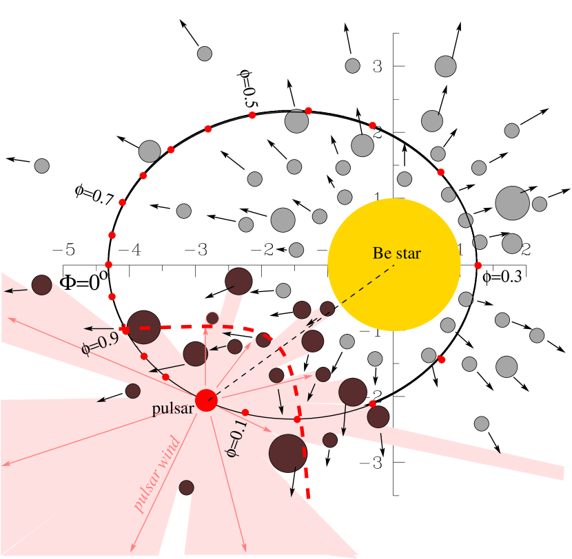
Figure 1: Schematic representation of interaction of the pulsar wind with a clumpy wind from companion Be star. Relativistic pulsar wind hits the nearest clumps of the stellar wind. Instead of a smooth bow-shaped contact surface (red dashed line) the interaction region (the set of the dark shaded clumps) is irregularly shaped. Ellipse represents correctly scaled pulsar binary orbit around the companion star. $x$ and $y$ axes are in units of the radius of companion star. Red dots along the orbit mark intervals regularly spaced in phase, $\Delta\phi=0.05$. The periastron corresponds to $\phi=0.3$ (Grundstrom et al., 2006).

2.3 Inhomogeneity of the stellar wind and short time scale variability of the source.

Long XMM-Newton observation of LSI +61^∘ 303 in 2005 has revealed variability of the system at $\Delta t\simeq(several)$ ks time scale, which is much shorter than the orbital period (Sidoli et al., 2006). Variability at a similar time scale is observed also in radio energy band (Peracaula et al., 1997). The observed variability indicates that the characteristics of interaction of the pulsar and stellar winds change at distance scales which are smaller than the size of the binary orbit. Distance scale relevant for the fast variability can be estimated as

$$R_{w}\sim v\Delta t\sim 10^{11}\left[\frac{v}{10^{7}\mbox{ cm/s}}\right]\left[\frac{\Delta t}{10\mbox{ ks}}\right]\mbox{ cm}$$ (1)

where $v$ is typical velocity scale (e.g. the orbital velocity of the pulsar, or the speed of the stellar wind).

If one assumes that the power output in the pulsar wind is constant, the distance scale related to the fast variability has to be associated with the pulsar wind interactions with inhomogeneities (clumps) of the stellar wind. Changes in the X-ray luminosity can be caused by the variaitons of the number of inhomogeneities exposed to the pulsar wind and/or variations of characteristics (density, size, magnetic field strength) of inhomogeneities.

As it is explained above, the inhomogeneity of the stellar wind leads the disappearence of a regular bow-shaped surface of pulsar/stellar wind interaction. The irregularity of the contact surface of wind interaction leads to a change in the regime of escape of high-energy particles from the vicinity of Be star. Namely, contrary to the the ”homogeneous wind” scenario, in which the shocked pulsar wind escapes along the bow-shaped contact surface in a time $t_{esc}\sim 3D/c\sim 30\left[10^{12}\mbox{ cm}/D\right]$ s (which depends on the distance $D$), the escape of the pulsar wind mixed with the stellar wind can slow down to

$$t_{esc}\sim D/v_{w}\sim 10^{5}\left[\frac{10^{12}\mbox{ cm}}{D}\right]\left[\frac{10^{7}\mbox{ cm/s}}{v_{wind}}\right]\mbox{ s}$$ (2)

The wind from the Be star is known to have anisotropic structure with a dense and ”slow” wind ($v_{w}\sim 10^{6}\div 10^{7}$ cm/s) in the equatorial region and rarefied ”fast” wind ($v_{wind}\sim(several)\times 10^{8}$ cm/s) from the polar regions. The difference in the escape time changes the balance between the synchrotron, IC and Coulomb energy losses of high-energy electrons injected in the region of interaction of pulsar and stellar winds.

2.4 Cooling of high-energy electrons in the clumps.

Following Maraschi & Treves (1981) and Chernyakova et al. (2006) we assume that X-ray emission from the system at energies $\epsilon_{IC}\sim 1-10$ keV is dominated by the IC scattering of optical photons from the Be star by electrons of energies about

$$E_{e,IC}\simeq 10\left[\frac{2\times 10^{4}\mbox{ K}}{T_{*}}\right]^{1/2}\left[\frac{\epsilon_{IC}}{4\mbox{ keV}}\right]^{1/2}\mbox{ MeV}$$ (3)

($T$ is the temperature of the Be star). Radio flux at the frequency $\nu_{synch}$ is produced via synchrotron emission from electrons with roughly the same energies,

$$E_{e,synch}\simeq 10\left[\frac{1\mbox{ G}}{B}\right]^{1/2}\left[\frac{\nu_{synch}}{7\mbox{ GHz}}\right]^{1/2}\mbox{ MeV}$$ (4)

($B$ is the magnetic field strength).

10 MeV electrons are injected in the inhomogeneities of the stellar wind irradiated by the relativistic pulsar wind. Such injection can be either the result of shock acceleration of electrons from the stellar wind or the result of cooling of higher energy electrons from the pulsar wind.

The high-energy particles can be retained in inhomogeneities with strong enough magnetic field. Assuming that electrons diffuse in disordered magnetic field, one can estimate the escape time (in the Bohm diffusion regime) as

$$t_{diff}\simeq 3\times 10^{6}\left[\frac{R_{w}}{10^{11}\mbox{ cm}}\right]^{2}\left[\frac{B}{1\mbox{ G}}\right]\left[\frac{10\mbox{ MeV}}{E_{e}}\right]\mbox{ s}$$ (5)

Comparing the escape time with the inverse Compton cooling time

$$t_{IC}(D,E_{e})\simeq 10^{4}\left[\frac{L_{*}}{10^{38}\mbox{ erg/s}}\right]\left[\frac{D}{10^{12}\mbox{ cm}}\right]^{2}\left[\frac{10\mbox{ MeV}}{E_{e}}\right]\mbox{ s}$$ (6)

($L_{*}$ is the luminosity of Be star) and/or synchrotron cooling time,

$$t_{synch}\simeq 3\times 10^{5}\left[\frac{1\mbox{ G}}{B}\right]^{2}\left[\frac{10\mbox{ MeV}}{E_{e}}\right]\mbox{ s}$$ (7)

one finds that if the magnetic field in the clump is $B_{clump}\sim 1$ G, then electrons captured in the clumps can efficiently cool before they escape.

The binary orbit of LSI +61^∘ 303 is very compact, so that at periastron the pulsar approaches the Be star as close as 1.3 stellar radii, $D\simeq 5\times 10^{11}$ cm (Grundstrom et al., 2006). Close to the surface of the star, not only the density of photon background is high, but also the density of the stellar wind, $n$. In this case 10 MeV electrons suffer from the strong Coulomb energy loss. The Coulomb loss time,

$$t_{Coul}\simeq 2\times 10^{3}\left[\frac{10^{10}\mbox{ cm}^{-3}}{n}\right]\left[\frac{E_{e}}{10\mbox{ MeV}}\right]\mbox{ s}$$ (8)

becomes shorter than the IC cooling time (6) below the ”Coulomb break” energy

$$E_{e,Coul}\simeq 20\left[\frac{L_{*}}{10^{38}\mbox{ erg/s}}\right]^{1/2}\left[\frac{D}{10^{12}\mbox{ cm}}\right]\left[\frac{n}{10^{10}\mbox{ cm}^{-3}}\right]^{1/2}\mbox{ MeV}$$ (9)

Most of the power injected in the form of electrons with energies below $E_{e,Coul}$ goes into heating of the stellar wind, rather than into the synchrotron and IC emission. If the density of the wind is

$$n>10^{10}\left[\frac{10^{12}\mbox{ cm}}{D}\right]^{2}\mbox{ cm}^{-3}$$ (10)

both the X-ray emission in the energy band $\epsilon_{IC}<10$ keV and radio emission below $\nu_{synch}\sim 10$ GHz (corresponding to $E_{e}\simeq 20$ MeV) are suppressed. In other words, the innermost part of the stellar wind is ”X-ray/radio dim”.

Radial gradients of the densities of the stellar wind and of the soft photon background lead to significant variations of the relative importance of Coulomb, IC and synchrotron energy losses with distance. This, in turn, leads to a complicated radial structure of the compact PWN.

2.5 Structure of the compactified pulsar wind nebula.

Recent VLBA monitoring of the source over an entire orbital cycle (Dhawan et al., 2006) reveals an extended radio source of a variable morphology with the overall size of $D_{PWN}\sim(several)\times 10^{14}$ cm which can be identified with a ”compactified” PWN, similar to the compactified PWN of PSR B1259-63 (Neronov & Chernyakova, 2006). The radio emission at 3-13 cm wavelengths (synchrotron photon energies $\epsilon_{synch}\sim(1\div 3)\times 10^{-5}$ eV) peaks outside the binary orbit, at the distance $D_{r}\sim(several)\times 10^{13}$ cm. The position of the peak moves around the central Be star on the orbital time scales.

The variability of morphology of the source on the orbital time scale shows that the cooling time of 10 MeV electrons responsible for the radio synchrotron emission is $t_{PWN}\leq 10^{6}$ s. Comparing this time with synchrotron and inverse Compton cooling times in the region of the size $D_{PWN}$ one can find that $t_{PWN}$ is shorter than the inverse Compton cooling time, $t_{IC}(D_{PWN},10\mbox{ MeV})$ (6). Equating $t_{PWN}\simeq t_{synch}$ (7) one can find the magnetic field strength in the compactified PWN, $B_{PWN}\simeq 1\mbox{~{}G}$.

Suppression of the radio synchrotron emission from the region $D<D_{r}$ can be explained by the fact that in the inner part of the PWN the inverse Compton energy loss dominates over the synchrotron loss. Indeed, from (6), (7) one can find that if the magnetic field in the nebula does not rise significantly toward the center, $t_{IC}<t_{synch}$ for the distances $D<10^{13}$ cm. Thus, the inverse Compton emission comes predominantly from the inner part of the nebula, while the synchrotron emission mostly comes from its outskirts.

High-energy electrons responsible for the radio and X-ray emission are initially injected in the region of interaction of the pulsar and stellar wind. Taking into account that the binary orbit of LSI +61^∘ 303 is very compact, $D_{orb}\sim(several)\times 10^{12}$ cm, one finds that the high-energy electrons can fill the entire compactified nebula before they loose all their energy on synchrotron emission only if they spread from the compact injection region with the speed $v\geq D_{PWN}/t_{synch}\simeq 10^{8}\mbox{ cm/s}$. There are two possibilities for such ”fast” escape. Either electrons travel with the nearly relativistic speed in the shocked pulsar wind, so that $v\sim 10^{10}$ cm/s, or they are injected into the nebula during the periods when the pulsar interacts with the clumps of the fast polar wind from Be star, which has the velocity $v_{wind}\geq 10^{8}$ cm/s.

In the former case it would be difficult to explain why the IC luminosity of the system is much higher than the synchrotron luminosity. Indeed, electrons would leave the compact region of the size $D<10^{13}$ cm in less than one kilosecond. This time is shorter than the IC cooling time and in such scenario most of the power of high energy electrons would be released via synchrotron, rather than via IC emission.

To the contrary, if electrons escape with the speed of the stellar wind, the periods of fast escape in the polar wind are intermittent with the periods of slow escape in equatorial wind. The velocity of the equatorial wind is $v_{wind}\sim 10^{6}\div 10^{7}$ cm/s. It takes electrons some $10^{6}$ s to escape to the distances beyond $10^{13}$ cm during the pulsar propagation through the equatorial wind. Since the escape time is larger than the IC cooling time in this case, most of the power is released via IC X-ray emission.

It is clear from the above discussion that the X-ray IC emission from the system is produced in the compact region, $D\leq 10^{13}$ cm, in the direct vicinity of the Be star. However, close to the stellar surface, electrons can suffer from the severe Coulomb loss. Since the radial profile of the density of the stellar wind in the equatorial disk, $n\sim D^{(-2)\div(-4)}$ (e.g. Waters et al. (1988)), is steeper than the soft photon density profile, $n_{ph}\sim D^{-2}$, the Coulomb loss can dominate over the IC loss in the innermost part of the compactified PWN. The X-ray IC emission from this innermost part is suppressed and most of the energy of 10 MeV electrons goes into heating of the stellar wind via Coulomb collisions.

Thus, the entire compactified PWN has the ”onion-like” structure shown in Fig. 2: in the innermost region of the nebula the dominant Coulomb loss suppresses both the IC and synchrotron luminosity, in the intermediate region $10^{12}$ cm$<D<10^{13}$ cm the IC energy loss dominates while in the outer part of the nebula $10^{13}$ cm$<D<(several)\times 10^{14}$ cm the synchrotron loss dominates.

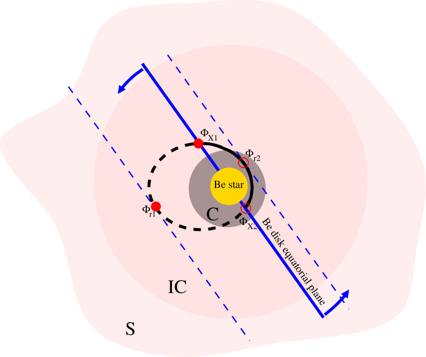
Figure 2: Onion-like structure of the compactified pulsar wind nebula of LSI +61^∘ 303. The Coulomb losses dominate in the innermost region marked as ”C”. The inverse Compton loss dominates in the region marked ”IC”. The synchrotron loss dominates in the outer region marked as ”S”. The ellipse shows the binary orbit. The suggested orientation of the equatorial plane of the geometrically thick Be star disk at the moment of 1996 RXTE observations is shown by the thick solid blue line. The part of the binary orbit behind the equatorial plane of Be star disk is shown by the dashed line. $\Phi_{X1}$ and $\Phi_{r1}$ mark the phases of maxima of X-ray and radio lightcurves (see text).

2.6 X-ray and radio lightcurves of the source.

X-ray (and radio) lightcurve of the system exhibit a single maximum per orbit, see Fig. 3. In this figure we plot the X-ray flux as a function of the ”angular” orbital phase, $\Phi$, defined in such a way that the apastron is at $\Phi=0^{\circ}$, while the periastron is at $\Phi=180^{\circ}$. The phase of the maximal X-ray flux is known to be shifted with respect to the maximum in radio band. Besides, the phases of X-ray and radio maxima shift from orbit to orbit. The overall variation of the X-ray flux from the system is by a factor of 2-3. The radio flux shows larger variations, by a factor of 10. The onion-like structure of the compactified PWN discussed in the previous subsection gives a clue to understand the behaviour of the X-ray and radio lightcurves.

The X-ray flux increases when the pulsar moves deeper into the slow equatorial wind of Be star. During these periods the high-energy electrons responsible for the X-ray emission are retained for a longer time in the vicinity of Be star where they efficiently loose energy via IC scattering. In such a model the maximum of the X-ray lightcurve at the phase $\Phi_{X1}\simeq 300^{\circ}$, observed with RXTE, has to be identified with the moment of the pulsar passage through the equatorial plane of the Be star disk (in 1996). This fixes the orientation of the disk is fixed as it is shown in Fig. 2.

Orbit-to-orbit fluctuations/shifts of the position of X-ray maximum are expected because the pulsar passes through the innermost part of the disk and the pulsar wind is injected into several individual clumps in the disk, rather than into the ”average” equatorial wind of Be star. Drift of the phase of X-ray maximum, $\Phi_{X1}$ on 4.6 yr year time scale of variability of Be star disk (Zamanov & Marti, 2000) is expected if e.g. the disk precesses or a significant asimutal inhomogeneity of the disk changes its orientation.

By analogy with the case of PSR B1259-63, one expects to find a second maximum of the X-ray lightcurve at the phase $(\Phi_{X2}=\Phi_{X1}-180^{\circ}\simeq 120^{\circ}$ (assuming the 1996 disk position), during the pre-periastron passage of the pulsar through the equatorial plane of Be star disk. However, during the second disk passage the pulsar is much closer to the surface of Be star, where the Coulomb loss can dominate over the IC loss. In this case most of the illuminated clumps of Be star wind are ”X-ray dim”, as it is explained in the previous sub-section. The decrease of amount of the X-ray bright clumps leads to the suppression of the second maximum of the X-ray lightcurve.

It is clear from the previous subsection that 10 MeV electrons can fill the entire compact PWN and efficiently emit synchrotron radiation in radio band only if they escape from the compact injection region with the speed $v\geq 10^{8}$ cm/s, much larger than the velocity of the equatorial wind. This leads to a suggestion that the radio luminosity of the system peaks during the period when the pulsar wind can be efficiently injected into the clumps of the polar wind of Be star. These period(s) correspond to the orbital phase when the pulsar moves to its highest position above or below the equatorial plane. (If the binary orbit would be circular, the phase of the radio maximum would be $\Phi_{r1}\simeq\Phi_{X1}+90^{\circ}$. The eccentricity of the orbit shifts the highest elevation above the disk to earlier or later phase. The phase of the radio maximum is found by drawing a tangent to the ellipse parallel to the assumed line of intersection of the orbital plane with the equatorial plane of Be star disk (the dashed lines in Fig. 2). Similarly to the case of X-ray lightcurve, the second maximum of the radio lightcurve, naively expected at $\Phi_{r2}$ (see Fig. 2), is missing because of the close approach of the binary orbit to the surface of Be star.

The phase of the maximum of the radio lightcurve is known to exhibit a periodic drift on the 4.6 yr timescale (Gregory et al., 2002). Within the proposed model, the drift of the radio maximum is associated to the drift of the phase of the highest elevation of the binary orbit above the equatorial plane of the Be star disk or, equivalently, of the orientation of the line of intersection of the equatorial plane of the Be star disk with the orbital plane. Such drift of the orientation of the line of intersection can be e.g. due to the precession of the disk with the period of 4.6 yr.

It is interesting to note that the pattern of the systematic 4.6 yr drift of the phase of the radio maximum agrees well with the assumption of the change of the mutual orientation of the orbital plane and the equatorial plane of Be star disk. Suppose that the line of intersection of the binary orbit with the equatorial plane of Be star disk rotates with a period of $P\simeq 2\times 4.6$ yr$\simeq 9.2$ yr. Suppose that at an initial moment the line of intersection of equatorial plane of Be star disk coincides with the major axis of the binary orbit. At this moment the phase of the maximal elevation of the binary orbit above the disk is roughly equal to $\Phi_{r1}\sim 290^{\circ}$ or $\Phi_{r1}\simeq 70^{\circ}$ (for the particular case of the binary orbit of LSI +61^∘ 303, see Fig. 1 and 2. If the line of intersection of the orbital plane with the equatorial plane of Be star disk precesses in the counter-clockwise direction, the phase of the highest elevation of the orbit above the equatorial plane of the disk grows from $\sim 290^{\circ}$ to $360^{\circ}$ and then further from $0^{\circ}$ to $\simeq 70^{\circ}$. In terms of the orbital phase, the phase of radio maximum changes from 0.45 to 1. and then from 0. to 0.1. At the moment when the line of intersection of orbital and equatorial plane again coincides with the major axis of the orbit, the phase of the radio maximum should make a “flip” from $\Phi_{r2}\simeq 70^{\circ}$ to $\Phi_{r1}\simeq 290^{\circ}$ (from $\phi\simeq 0.1$ to $\phi\simeq 0.45$). Since the line of intersection of orbital and equatorial planes coincides with the major axis twice per period, the “flips” of the phase of radio maximum are expected to happen with a period of $P/2\simeq 4.6$ yr. Long term radio monitoring of the system (Gregory et al., 2002) shows that indeed the phase of the radio maximum drifts from $\phi\simeq 0.45$ to $\phi\simeq 1.$ and subsequently flips from $\phi\simeq 0.1$ to $\phi\simeq 0.45$ with periodicity of $4.6$ yr. The radio maximum never appears within $0.1<\phi<0.4$, in good agreement with the proposed explanation in terms of the phase of the highest elevation of the binary orbit above the equatorial plane of Be star disk.

2.7 $\gamma$-ray lightcurve.

Electrons responsible for the TeV $\gamma$-ray emission from the system are not able to fill the whole volume of the compactified PWN because of the very short cooling time. The shortest cooling time is achieved at electron energies $E_{e}\sim 10-100$ GeV, $t_{IC}(10^{12}\mbox{ cm},10\mbox{ GeV})\simeq 10$ s (see Eq. (6)). The IC scattering on 100 GeV – TeV electrons proceeds in the Klein-Nishina regime. In this regime the electron cooling time grows with energy

$$t_{IC(KN)}\simeq 10^{2}\left[\frac{L_{*}}{10^{38}\mbox{ erg/s}}\right]\left[\frac{\epsilon_{IC}}{1\mbox{ TeV}}\right]^{0.7}\left[\frac{D}{10^{12}\mbox{ cm}}\right]^{2}\mbox{ s}$$ (11)

Propagation of electrons with the energy about 100 GeV is affected by development of the pair production cascade in the field of soft photons from Be star (with typical energy $\epsilon_{*}\sim 1-10$ eV). The density of such photons is

$$n_{ph}\sim 10^{13}\left[\frac{L_{*}}{10^{38}\mbox{ erg/s}}\right]\left[\frac{10^{12}\mbox{ cm}}{D}\right]^{2}\mbox{ cm}^{-3}$$ (12)

Taking into account that the pair production cross-section peak at the value $\sigma_{\gamma\gamma}\simeq 10^{-25}$ cm² for $\gamma$-rays of energy $E_{\gamma}\simeq\left[10\mbox{ eV}/\epsilon_{*}\right]100\mbox{ GeV}$, one can estimate the optical depth for the 100 GeV – 1 TeV $\gamma$-rays as

$$\tau_{\gamma\gamma}\simeq 1\left[\frac{L_{*}}{10^{38}\mbox{ erg/s}}\right]\left[\frac{10^{12}\mbox{ cm}}{D}\right]$$ (13)

The life time of both 100 GeV-TeV and 10 GeV electrons is much shorter than the escape time to the region of dominance of synchrotron loss, $D\geq 10^{13}$ cm. The cascade electrons and positrons loose energy mostly via IC (rather than via synchrotron) emission. This means that development of electromagnetic cascade efficiently channels the power initially injected into 100 GeV – TeV energy band to the energy band around $\sim 10$ GeV.

Since the optical depth with respect to the pair production is highest near the periastron, one expects to observe a ”deep” in the 100 GeV – TeV lightcurve of the source around the phases $\Phi\sim 180^{\circ}$ ($\phi\sim 0.3$) in agreement with MAGIC observations (Albert et al., 2006). The shape of the source lightcurve in the energy band below $\sim 10$ GeV should be qualitatively different from the one in the 100 GeV-TeV energy band. Since (a) the $10$ GeV emission is not uppressed by the pair production and (b) a part of the $10$ GeV power is generated via the development of electromagnetic cascade in the source, the maximum of the 10 GeV flux is expected roughly during the phases of maximal suppression of the 100 GeV-TeV flux. In other words, future observations of the source with AGILE and GLAST are expected to find a maximum, rather than minimum of the 1-10 GeV lightcurve around the phases $\Phi\sim 180^{\circ}(\phi\sim 0.3$).

2.8 Model summary.

To summarize, we find that the “compactified PWN” model can explain all observational properties of LSI +61^∘ 303, from radio to TeV $\gamma$-ray energy band. The main assumption of this model is that the nebula has an ”onion-like” structure. The inner region of the nebula at $D<10^{12}$ cm is characterized by the dense stellar wind and dense photon background. In this region the 10 MeV electrons, responsible for the radio and X-ray emission loose energy mostly on heating of the stellar wind, while 100 GeV-TeV electrons initiate the development of pair cascades. This explains the suppression of the radio, X-ray and TeV $\gamma$-ray luminosity of the source close to the periastron. The X-ray luminosity peaks when the pulsar moves out of the dense central part into the intermediate region $D>10^{12}$ cm where the dominant energy loss mechanism is the IC scattering of soft photons from Be star. The radio luminosity reaches its maximum during the phases when 10 MeV electrons are efficiently supplied by the fast polar wind from Be star to the outermost part of the nebula, $D>10^{13}$ cm, where the synchrotron loss dominates.

Qualitative analysis of behaviour of the X-ray and radio lightcurves of the system has enabled us a tentative determination of the orientation of the equatorial plane of the wind from Be star (at the moment of 1996 RXTE observations), in which the density of the stellar wind is highest. Since the correlation of the maximum of X-ray lightcurve with the moment of the pulsar passage through the middle of the disk is one of the key points of our model, it is interesting to find a confirmation for this fact in experimental data.

A complimentary information about the orientation of the binary orbit with respect to the Be star disk can be obtained from the observation that the passage of the pulsar from below to above (from the point of view of observer on the Earth) the densest part of the disk is associated with the decrease of the column density of matter between the position of the pulsar and the observer. Passage of the pulsar from above to below the densest part of the disk is then associated with the rise of the column density. Taking into account that the estimated density of the stellar wind in the most compact part of the PWN is $n>10^{10}$ cm^-3, while the thickness of the dense layer of the wind is about the size of the star, $\sim R_{*}\sim(several)\times 10^{11}$ cm, one expects to find the variations of the matter column density

$$\Delta N_{H}\sim nR_{*}\geq 10^{21}\mbox{ cm}^{-2}$$ (14)

Such variations are, in principle, detectable by XMM-Newton.

As it is mentioned above, in our model the suppression of the X-ray maximum during the pre-periastron passage of the pulsar through the densest part of the Be star disk is explained by the dominance of the Coulomb loss in the innermost part of the stellar wind. The dominance of the (energy independent) Coulomb loss leads to hardening of electron spectrum which, in turn, should lead to the hardening of IC emission spectrum which is also a potentially detectable effect.

In the following section we make an attempt to find both the variation of $N_{H}$ and the hardening of the spectrum associated to the pulsar passage through the densest part of the disk in the available observational data on LSI +61^∘ 303. The re-analysis of experimental data allows us to further constrain the geometry of the system (in particular, its orientation with respect to the line of sight).

3 Re-analysis of the archive X-ray data.

In the previously published analysis of the available X-ray data, the hydrogen column density was fixed during the model fitting of the data, so that no information about presence/absence of the short and long time scale variations of $N_{H}$ is available. The main reason for this is the difficulty of ”disentanglement” of variations of $N_{H}$ from the variations of the photon index, $\Gamma$, in the commonly accepted X-ray spectral model of the source, which consists of a powerlaw spectrum modified at low energies by the photo-absorption. Since the variations of $N_{H}$ by $(several)\times 10^{21}$ cm^-2 are only marginally detectable with such instruments as XMM-Newton, all previously published analyses assumed for simplicity a constant value of $N_{H}$.

The set of available X-ray data considered in our re-analysis consists of the monitoring of the source over a single orbital cycle with RXTE (Harrison et al., 2000), five short XMM-Newton 2002 observations (Chernyakova et al., 2006) and a long (50 ks) 2005 XMM-Newton observation (Sidoli et al., 2006). Table 1 gives a summary of the observations analyzed below.

Table 1: Journal of RXTE observations of LSI +61^∘ 303

Date	Exposure	Orbital	$\Gamma$	Flux(2-10 keV)	$\chi^{2}(dof)$
	(ks)	Phase		($\times 10^{-11}$ ergs cm-2s-1)
1996 Mar 01 13:57-19:25	7.9	0.79	1.65${}_{-0.12}^{+0.10}$	1.17${}_{-0.21}^{+0.24}$	16.93(23)
1996 Mar 04 21:38-01:36	8.0	0.90	1.72${}_{-0.09}^{+0.08}$	1.49${}_{-0.20}^{+0.23}$	11.61(23)
1996 Mar 07 23:33-03:28	7.9	0.01	1.86${}_{-0.13}^{+0.12}$	0.99${}_{-0.20}^{+0.22}$	26.09(48)
1996 Mar 10 01:07-05:02	7.7	0.11	1.83${}_{-0.12}^{+0.16}$	0.94${}_{-0.17}^{+0.28}$	14.79(23)
1996 Mar 13 04:06-08:19	8.7	0.23	1.55${}_{-0.11}^{+0.10}$	1.15${}_{-0.19}^{+0.22}$	17.10(23)
1996 Mar 16 00:54-06:06	8.3	0.34	1.62${}_{-0.08}^{+0.08}$	1.62${}_{-0.21}^{+0.22}$	25.16(48)
1996 Mar 18 10:44-15:48	8.3	0.43	1.56${}_{-0.06}^{+0.06}$	2.15${}_{-0.20}^{+0.23}$	19.67(23)
1996 Mar 24 07:55-13:10	10.2	0.65	1.93${}_{-0.10}^{+0.09}$	1.17${}_{-0.17}^{+0.19}$	17.20(20)
1996 Mar 26 00:56-06:46	12.3	0.71	1.84${}_{-0.11}^{+0.10}$	1.06${}_{-0.17}^{+0.19}$	16.99(20)
1996 Mar 30 04:07-10:40	12.9	0.87	1.89${}_{-0.11}^{+0.10}$	0.93${}_{-0.16}^{+0.17}$	16.50(20)

3.1 RXTE/PCA observations

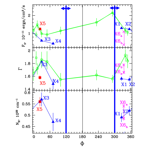
Figure 3: Spectral variability of the system in 2-10 keV energy range, as observed with XMM-Newton (red, blue and magenta points) and RXTE (green open squares). Observations done during one and the same orbital cycle are connected with a line. The time is assumed to increase from left to right. Vertical thick blue lines show the suggested position of intersection of equatorial plane of the Be star wind with the binary orbit at the moment of 1996 RXTE observations. Thin black vertical line marks the position of periastron ($\Phi$=180).

In 1996 RXTE has closely monitored LSI +61^∘ 303  making 11 observations along the single orbit, see Table 1. For the first time these data were presented in the paper of Harrison et al. (2000) where the authors report that no significant variability of the spectral shape is visible in RXTE data. Our reanalysis of the RXTE data with the latest LHEASOFT 5.2 provided by the RXTE Guest Observer Facility reveals, to the contrary, a systematic variation of the spectrum along the orbit. Namely, the rise of X-ray flux is associated to the hardening of the spectrum with the photon index decreasing from $\Gamma\simeq 1.9$ down to $\Gamma\simeq 1.5$.

The results of our spectral analysis performed with XSPEC v 11.3.2 are given in Table 1, and are graphically represented in the Fig. 3. The line of intersection of the equatorial plane of the Be star disk with the orbital plane (at the moment of RXTE observations), suggested from the qualitative considerations of the previous section, is shown by the vertical blue lines shifted by $\Delta\Phi=180^{\circ}$. The orientation of the disk is chosen in such a way that the maximum of RXTE lightcurve at $\Phi_{X1}\simeq 300^{\circ}$ corresponds to the moment of the pulsar passage through the equatorial plane of the disk (in general, the disk is geometrically thick, so the pulsar can spend most of its orbit inside the disk). As it is discussed in the previous section, the second maximum, at $\Phi_{X2}\simeq 120^{\circ}$ is suppressed because the pulsar passes closer to the Be star where the disk is so dense that most of the power of high-energy electrons injected in the disk goes onto Coulomb heating of the disk, rather than on the IC X-ray emission. From the middle panel of Fig. 3 one can clearly see that the suggested moment of the pre-periastron passage of the equatorial plane at $\Phi_{X2}\simeq 120^{\circ}$ is associated with the hardening of the X-ray spectrum of the system.

Unfortunately, the PCA data do not allow one to find unambiguously the true value of hydrogen column density $N_{H}$, because of the lack of sensitivity at the energies below 3 keV. Only the information about the variations of photon index, $\Gamma$, is available. For the purpose of the model fit we have fixed the value $N_{H}=0.49\times 10^{22}$ cm^-2 derived by Chernyakova et al. (2006) from 2002 XMM-Newton data.

3.2 XMM-Newton observations

XMM-Newton has observed LSI +61^∘ 303 with the EPIC instruments five times during 2002, and once in 2005. Four 2002 observations have been done during the same orbital cycle, and the fifth one has been done seven months later. The log of the XMM-Newton data discussed in this paper is presented in Table 2. These data have already been analyzed in papers of Chernyakova et al. (2006) and Sidoli et al. (2006). In these works it was shown that simple power law with photoelectric absorption describes the spectrum of LSI +61^∘ 303 well, with no evidence for any line features.

Table 2: Journal of XMM-Newton observations of LSI +61^∘ 303

Data	Observational	Date	MJD	Orbital	Exposure (ks)
Set	ID		(days)	Phase
X1	0112430101	2002-02-05	52310	0.55	6.4
X2	0112430102	2002-02-10	52315	0.76	6.4
X3	0112430103	2002-02-17	52322	0.01	6.4
X4	0112430201	2002-02-21	52326	0.18	7.5
X5	0112430401	2002-09-16	52533	0.97	6.4
X6	0207260101	2005-01-27	53397	0.61	48.7

The XMM-Newton Observation Data Files (ODFs) were obtained from the on-line Science Archive; the data were then processed and the event-lists filtered using xmmselect within the Science Analysis Software (sas) v6.0.1. We re-analyzed the XMM-Newton observations using the methods described in Chernyakova et al. (2006).

Table 3: Spectral parameters for XMM-Newton Observations of LSI +61^∘ 303.^∗

Data	$F$(2-10 keV)	$\Gamma$	$N_{H}$	$\chi^{2}$ (dof)
Set	$10^{-11}$erg s-1		($10^{22}$ cm-2)
X1	1.30$\pm 0.02$	1.60$\pm 0.03$	0.49$\pm 0.02$	261(264)
X2	1.24$\pm 0.03$	1.55$\pm 0.03$	0.52$\pm 0.02$	272(252)
X3	0.60$\pm 0.03$	1.83$\pm 0.05$	0.57$\pm 0.03$	182(165)
X4	0.44$\pm 0.03$	1.48$\pm 0.08$	0.47$\pm 0.04$	70(76)
X5	1.25$\pm 0.03$	1.58$\pm 0.03$	0.56$\pm 0.02$	277(284)
X6a	1.10$\pm 0.02$	1.66$\pm 0.02$	0.54$\pm 0.01$	653(649)
X6b	0.37$\pm 0.01$	1.78$\pm 0.02$	0.49$\pm 0.01$	435(458)

^∗ Given errors represent 1$\sigma$(68.3%) confidence interval uncertainties.

Figure 4: Confidence contour plots of the column density $N_{H}$ and of the photon spectral index $\Gamma$ uncertainties for a power-law fit to XMM-Newton observations. The contours give 1$\sigma$ (68.3%) and 2$\sigma$ (95.4%) confidence levels.

The results of our spectral analysis are given in Table 3 and Fig. 3. Following the work of Sidoli et al. (2006) we have split observation X6 into two, X6_a and X6_b. X6_a corresponds to the first 20 ks of the observations, and X6_b to the rest.

3.3 Systematic variation of X-ray spectrum along the orbit.

From the bottom panel of Fig. 3 one can see a hint of systematic variation of $N_{H}$ over the orbit (the probability of non-variable $N_{H}$ is 0.02%). From observations X1 – X5 one can guess that the column density appears to be lower around the orbital phases closer to periastron and higher at apastron. At the same time, the variation of $N_{H}$ at 50 ks scale during the observation X6 is comparable to the scatter of $N_{H}$ values on the orbital time scale. Obviously, more observations, especially around the periastron, $120^{\circ}<\Phi<240^{\circ}$ would help to clarify the question of the systematic orbital modulation of equivalent hydrogen column density.

A possible interpretation of the orbital modulation of $N_{H}$ is that the part of the binary orbit around the periastron is situated closer to observer. In this case the part of the orbit around the apastron is embedded ”deeper” into the stellar wind, from the viewpoint of observer and photons have to pass through a higher matter column density.

The middle panel of Fig. 3 shows the orbital evolution of the photon index $\Gamma$. One can see that a spectral hardening similar to the one found in RXTE data is observed at the phases $\Phi\sim 120^{\circ}$ (suggested pre-periastron passage of the equatorial plane of the disk). However, contrary to the RXTE observations, no softening of the spectrum is observed after the phase $\Phi_{X1}\simeq 300^{\circ}$. In general, a large scatter of the values of X-ray flux and photon indexes are found at the phases $\Phi>300^{\circ}$. This can be explained either by physical arguments (close to the apastron the density of clumps in the stellar wind decreases which leads to the significant variability of the flux and the spectral index), or, possibly, by the low quality of X-ray data (the precision of the measurements can be insufficient to measure independently $N_{H}$ and $\Gamma$).

To address this question in more details, and to avoid the possible degeneracy on the determination of the photon index and column density we show in Fig. 4 the 1$\sigma$ and 2$\sigma$ confidence levels contour plots of spectral index $\Gamma$ versus $N_{H}$. From this figure one can see that un-freezing of $N_{H}$ in the model fit does not prevent the detection of variability of $\Gamma$ over the orbit.

3.4 Short time scale variations of $N_{H}$.

The long XMM-Newton observation of the system in 2005 as well as radio observations by Peracaula et al. (1997) reveal the variability of the flux from the system on the time scales of several kiloseconds. Interpretation of the short time scale variability in the model of interaction of the pulsar wind with the clumps of the stellar wind suggests that both the photon index $\Gamma$ and the column density $N_{H}$ should vary at this time scale.

To study the possible short time scale variability of both $N_{H}$ and $\Gamma$ we have split the long XMM-Newton observation onto time bins of duration of 2 ks, extracted the spectrum of the source separately in each time bin and fitted it with the absorbed powerlaw model. The resulting dependence of the column density $N_{H}$ and the photon index $\Gamma$ on the flux from the source is shown in top and bottom panels of Fig. 5.

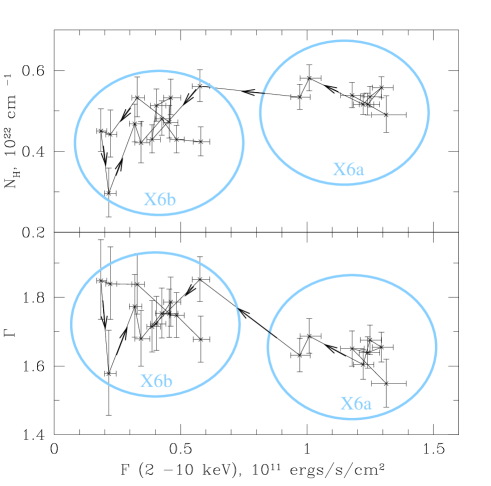
Figure 5: Column density (top panel) and spectral slope (bottom panel) dependence on the 2 - 10 keV Flux during the X6 observation with a bin time of 2000 s. Arrows show the direction of time evolution.

In the top panel of Fig. 5 one can see that the column density decreases when the flux drops. The probability that $N_{H}$ was constant during the whole 50 ks observation is less than 0.03%. Such behaviour is natural to expect within the ”clumpy wind” model: lower density of the clumps and/or smaller number of active (i.e. illuminated by the pulsar wind) clumps should result in the lower luminosity of the system.

Bottom panel of Fig. 5 shows the dependence of the spectral index $\Gamma$ on the 2 - 10 keV flux. Softening of the spectrum is observed during the period of a lower flux values. Such behaviour is also expected in the ”clumpy wind” model: cooling of high-energy electrons at the end of activity of a clump leads to the softening of the spectrum of IC emission, as it is discussed in Chernyakova et al. (2006).

3.5 High and low flux spectral states of the source.

The direction of the time evolution in Fig. 5 is shown with arrows. In both panels data points clearly split into two groups, corresponding to X6a (group of points on the right with high flux), and X6b (group of points on the left with low flux) observations on the Fig. 3. The qualitative behaviour of the system is somewhat different in the ”high flux” and ”low flux” state. In the ”high flux” state the characteristics of the system ”stabilize”, in the sense that a well defined value of the photon index, close to $\Gamma\simeq 1.5$, and of $N_{H}$, close to $N_{H}\simeq 0.5\times 10^{22}$ cm^-2, are found. To the contrary, in the ”low flux” state the systems exhibits an irregular behaviour, with significantly variable $N_{H}$ and $\Gamma$.

To test the distinction between the low and high flux states we have investigated the spectral evolution of the system on the 1 ks time scale also in the 5 short XMM-Newton observations. Fig. 6 shows the results of our analysis. To make the definition of the ”spectral state” of the system independent of the model used to fit the spectrum, we plot in this figure the model-independent ”hardness ratio”, as a function of the X-ray flux. One can see that indeed, in the ”high flux” state, the hardness ratio does not exhibit significant variations, which signifies that the spectrum of the system is stable. To the contrary, the ”low flux” states can be divided onto ”low soft” and ”low hard” states, corresponding to the different values of the hardness ratio.

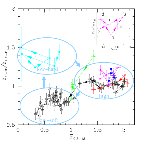
Figure 6: Hardness ratio versus count rate in the 0.3-12 keV energy range for all XMM-Newton observations (EPIC pn) of the source, with a bin time of 1000 s. The hardness ratio is defined as ratio between counts in the hard 2-12 keV and soft 0.3-2 keV energy range. Open red squares correspond to observation X1, filled blue circles to X2, open green triangles to X3, cyan filed squares to X4, filled magenta triangles to X5, and open black circles to X6. Arrows show the direction of time evolution. The enlarged view of the X5 observation is shown on the inset.

The pattern of the source variability in the ”hardness ratio vs. flux” diagram turns out to be qualitatively different from the pattern observed in conventional accreting X-ray binaries (Zdziarski et al., 2004). Namely, the spectral evolution proceeds along the ”high-hard” $\rightarrow$ ”intermediate-soft” $\rightarrow$ ”low-soft” $\rightarrow$ ”low-hard” $\rightarrow$ ”high-hard” loop. This loop is exactly opposite to the ”low-hard” $\rightarrow$ ”intermediate-soft” $\rightarrow$ ”high-soft” $\rightarrow$ ”intermediate-hard” $\rightarrow$ ”low-hard” evolution loop observed in accretion powered X-ray binaries.

The observed evolution pattern in the hardness ratio vs. flux diagram can be naturally explained in the compactified PWN model of the source. A stationary spectrum of the ”high” state is achieved when a sufficiently large number of the stellar wind clumps is illuminated by the pulsar wind. Drop of injection of the high-energy electrons at the end of activity of the clumps leads to the softening of the X-ray spectrum during the flux decrease. Hard spectrum in the low flux state is achieved during the pulsar passage through the densest part of the stellar wind.

3.6 Mini-flares produced by activity of individual clumps.

The short, kilosecond time scale, variability of $N_{H}$ can be associated with the variations of the density of the stellar wind from clump to clump. Indeed, if the typical density of the clump is $n\sim 10^{10}$ cm^-3, while its size is $R_{clump}\sim 10^{11}$ cm, one expects to find the fluctuations of the column density $\delta N_{H}\sim nR_{clump}\sim 10^{21}$ cm^-2 when the activity of individual clumps switches on/off.

The activity of individual clumps results in the short, several kilosecond, ”mini-flares” observed in the X-ray data. Examples of such ”mini-flares” are visible e.g. in the XMM-Newton observations X6b and X5 which is shown in more details in the inset in the right top corner of Fig. 6 and in Fig. 7. Similarly to the case of the long XMM-Newton observation, we split the whole observation X5 into 6 intervals of duration of 1 ks and extract the spectra of the source separately in each interval. One can see that the X-ray flux started to grow during the second ks interval, reached its maximum in the 5th interval and subsequently dropped to its initial value during the interval 6. The column density $N_{H}$ started to grow exactly at the moment of the on-set of the mini-flare, during the interval 2 and continued to grow until the flux reached its highest value during interval 5. The scale of the variation of $N_{H}$ during the mini-flare enables to estimate the column density of the clump responsible for the flare, $N_{H,clump}\simeq 10^{21}$ cm^-2. Remarkably, the spectrum of the source hardened on the time scale of 1 ks at the moment of the onset of the mini-flare (period 2) and stabilized at the value $\Gamma\simeq 1.6$ afterwards. Such transient hardening of the spectrum on the time scale shorter than the inverse Compton cooling time (6) can be explained by the fact that the equilibrium electron spectrum determined by the balance of injection and cooling rates is established only at the time scales of about $t_{IC}$ (6).

Figure 7: Confidence contour plots ( 1$\sigma$ level) of the column density $N_{H}$ and of the photon spectral index $\Gamma$ uncertainties for a power-law fit to each 1000 s of X5 observation.

4 Conclusions.

We have developed a model of the ”compactified” pulsar wind nebula of the $\gamma$-ray-loud binary system LSI +61^∘ 303. It turns out that this model can explain the observed properties of the source in radio, X-ray and $\gamma$-ray energy bands. In this model the maximum of the X-ray flux from the source is reached when pulsar crosses the middle plane of the dense equatorial wind from Be star. Maximum of the radio emission is achived when the pulsar wind penetrates most efficiently into the region of fast polar wind from Be star. Maximal luminosity in 100 GeV-TeV energy band is achieved when the propagation of very-high energy $\gamma$-rays is least affected by the pair production. The naively expected maxima of X-ray and radio lightcurves close to the phase of periastron of the binary orbit are suppressed because of the dominance of Coulomb loss inside the densest part of the stellar wind.

Association of the observed X-ray maximum with the period of the pulsar passage through the densest part of the disk has enabled us to constrain the orientation of the binary orbit with respect to the anisotropic wind from Be star. To test the conjecture about the orientation of the binary orbit we have searched for the variations of the hydrogen column density (which can be associated with the pulsar passage through the dense part of the stellar wind) in the available X-ray data. We find a marginally detected orbital variation of $N_{H}$. This orbital variation of $N_{H}$, if confirmed with more X-ray observations around the periastron, constrains also the orientation of the system with respect to the line of sight.

Our re-analysis of available X-ray observations of LSI +61^∘ 303 has also revealed that the changes in the spectral state of the source are accompanied by the changes in the hydrogen column density by $\Delta N_{H}\sim 10^{21}$ cm^-2, not only on the long (orbital) time scale, but also on the short (several kilosecond) time scale. This supports the hypothesis that the short, kilosecond time scale variations of the source flux are caused by the motion of compact object through the dense clumps of wind from the companion Be star.

5 Acknowledgments

The authors would like to thank M. Revnivtsev for the help with RXTE data analysis. We are also grateful to V.Bosch-Ramon for useful discussions of the subject.

References

- Albert et al. (2006) Albert J., et al., 2006, Science, 312, 1771.
- Bosch-Ramon et al. (2006) Bosch-Ramon, V.; Paredes, J. M.; Romero, G. E.; Ribo, M. 2006, A&A, 459, L25.
- Chernyakova et al. (2006a) Chernyakova M., Neronov A., A. Lutovinov, J. Rodriguez, S. Johnston, 2006a, MNRAS, 367, 1201.
- Chernyakova et al. (2006) Chernyakova M., Neronov A., Walter R., 2006, MNRAS, 372, 1585.
- Dubus (2006) Dubus G., 2006, accepted to A&A, astro-ph/0605287
- Dhawan et al. (2006) Dhawan, Mioduszewski, Rupen, 2006, in Proc. of VI Microquasar Workshop, Como-2006
- Gregory et al. (2002) Gregory P.C. 2002, ApJ, 575, 427
- Gregory et al. (1999) Gregory P.C., Peracaula M., Taylor A.R., 1999, ApJ, 520, 376
- Grundstrom et al. (2006) Grundstrom E. D. et al., 2006, accepted to ApJ (astro-ph/0610608)
- Harrison et al. (2000) Harrison F., Ray P.S., Leahy D., Waltman E.B., Pooley G.G., 2000, ApJ, 528, 454
- Johnston et al. (1992) Johnston S., Manchester R.N., Lyne A., Bailes M., Kaspi V. M., Qiao Guojun, D’Amico N., 1992, ApJ ,387, L37
- Maraschi & Treves (1981) Maraschi L., Treves A., 1981, MNRAS, 194, 1
- Mirabel & Rodriguez (1999) Mirabel I.F.,Rodriguez L.F., 1999, ARA&A, 37, 409.
- Neronov & Chernyakova (2006) Neronov A., Chernyakova M., 2006, Ap.S.S., accepted [astro-ph/0610139].
- Peracaula et al. (1997) Peracaula M., Marti J., Paredes J.M., 1997, A&A, 328, 283
- Puls et al. (2006) Puls J., Markova N., Scuderi S., Stanghellini C., Taranova O.G., Burnley A.W., Howarth I.D., 2006, A&A 454, 625.
- Romero et al. (2005) Romero G.E., Christiansen H. R., Orellana M., 2005, Ap.J., 632, 1093
- Sidoli et al. (2006) Sidoli L., Pellizzoni A., Vercellone S., Moroni M., SMereghetti S., Tavani M., 2006, A&A, 459, 901
- Taylor & Gregory (1984) Taylor A.R., Gregory P.C., 1984, ApJ, 283, 273
- Tavani & Arons (1997) Tavani M. & Arons J., 1997, Ap.J., 477, 439
- Waters et al. (1988) Waters L.B.F.M., van den Heuvel E. P. J., Taylor, A. R., et al., 1988, A&A, 198, 200
- Zamanov & Marti (2000) Zamanov R.K., Marti J., 2000, A& A, 358, L55
- Zdziarski et al. (2004) Zdziarski A., Gierlinski M., Mikolajewska J., Wardzinski G., SMith D., Harmon A., Kitamoto S., 2004, MNRAS, 351, 791.