MHD evolution of a fragment of a CME core in the outer solar corona

Abstract

Context. Detailed hydrodynamic modeling explained several features of a fragment of the core of a Coronal Mass Ejection observed with SoHO/UVCS at $1.7$ $R_{\odot}$ on 12 December 1997, but some questions remained unsolved.

Aims. We investigate the role of the magnetic fields in the thermal insulation and the expansion of an ejected fragment (cloud) traveling upwards in the outer corona.

Methods. We perform MHD simulations including the effects of thermal conduction and radiative losses of a dense spherical or cylindrical cloud launched upwards in the outer corona, with various assumptions on the strength and topology of the ambient magnetic field; we also consider the case of a cylindrical cloud with an internal magnetic field component along its axis.

Results. We find that a weak ambient magnetic field ($\beta\sim 20$) with open topology provides both significant thermal insulation and large expansion. The cylindrical cloud expands more than the spherical one.

1 Introduction

The study of Coronal Mass Ejections (CME) has received a strong impulse since the launch of the Solar Heliospheric Observatory (SoHO) in 1995 (Domingo & Poland, 1988). The Ultraviolet Coronal Spectrometer (UVCS) on board SoHO (Kohl et al., 1995) monitored the evolution of many CMEs and brought detailed spectroscopic information on plasma in CMEs during their propagation in the outer corona.

Ciaravella et al. (2000) and Ciaravella et al. (2001) analyzed in detail a CME occurred on 12 December 1997. Ciaravella et al. (2001) addressed more specifically the features observed at a distance of about $2$ $R_{\odot}$ by SoHO/UVCS, and hydrodynamic (HD) simulations of a cloud expelled out of the corona were performed to investigate which features of a fragment of the CME core observed with SoHO/UVCS could be explained in terms of purely HD effects. That model assumed the CME fragment to be already formed and launched with an initial impulse, and studied its evolution while traveling from the height of the EIT observation ($\sim 1.2$ $R_{\odot}$) to that of the UVCS observation ($\sim 1.7$ $R_{\odot}$). The HD model was able to reproduce various features observed in SoHO/UVCS UV lines (C III and O VI). The fragment was constrained to be initially denser than its surrounding with a density contrast $\delta n/n_{0}\sim 3$ and the background density to be $\sim 10^{8}$ $cm^{-3}$.

From the results of HD modeling, Ciaravella et al. (2001) argued that the thermal insulation of the core fragment is required to explain its evolution and to fit the UVCS observation. However, two main questions remained open. First, the thermal insulation needs to be physically motivated, since the thermal conduction is very efficient in the corona; in particular numerical simulations showed that the CME fragment thermalizes with the hot atmosphere on a very short time scale unless the thermal conduction is somehow suppressed. Second, the CME is observed to expand by a factor 3 to 4 in diameter (Ciaravella et al., 2000) traveling from the low corona to the height of the UVCS observation, while the hydrodynamic simulations lead to a smaller expansion of the fragment. Although the modeling suggests that very elongated structures may expand more, the amount of expansion needs further investigation.

Here, we extend the modeling study described in Ciaravella et al. (2001) and investigate whether magnetic fields may have a crucial role to answer the questions left open in the previous study, i.e. the thermal insulation and/or the amount of the expansion of the moving CME fragment. The magnetic field is able to funnel the thermal conduction, and it may lead to a strong thermal insulation of the fragment depending on the magnetic field topology. For this purpose, we revisit the modeling approach described in Ciaravella et al. (2001) now including an ambient magnetic field and using a full MHD modeling that includes non-isotropic thermal conduction, to understand in which conditions the expelled fragment can be thermally insulated or may expand more. We study the evolution of the moving fragment for different topologies and intensities of the ambient coronal magnetic field, and eventually consider also a fragment with an internal magnetic field, therefore accounting for the ejection of magnetic flux. In section 2 we describe the model, section 3 presents the simulations and in section 4 we discuss the results.

2 The model

Our scope is to study the evolution of an ejected CME core fragment as it travels through the high corona, extending the modeling described in Section 5.2 of Ciaravella et al. (2001). Again, we consider a simplified model of a plasma cloud, denser than the surrounding atmosphere and moving upwards in a stratified atmosphere with parameters that lead to the conditions observed at $1.7$ $R_{\odot}$ with UVCS. At variance with Ciaravella et al. (2001) now we consider the presence of an ambient magnetic field. We model the fragment while it travels in a $\beta\ga 1$ environment (Gary, 2001), where we cannot neglect the magnetic pressure, nor the thermal one, and we include the effect of the solar gravity, the radiative losses from an optically thin plasma, a coronal heating (needed to keep the unperturbed atmosphere in hydrostatic conditions), and the anisotropic thermal conduction in the presence of a magnetic field.

For continuity with the work of Ciaravella et al. (2001), we will first report on the evolution of a plasma cloud moving in various configurations of ambient magnetic field and eventually consider the case of a cloud of magnetic flux and plasma, i.e. a “magnetized” cloud, with an internal magnetic field.

We solve the ideal MHD equations (here in CGS conservative form):

$$\frac{\partial\rho}{\partial t}+\@vec{\nabla}\cdot(\rho\@vec{v})=0$$ (1)

$$\frac{\partial\rho\@vec{v}}{\partial t}+\@vec{\nabla}\cdot(\rho\@vec{v}\@vec{v})=-\nabla p+\frac{(\@vec{\nabla}\times\@vec{B})\times\@vec{B}}{4\pi}+\rho\@vec{g}$$ (2)

$$\frac{\partial u}{\partial t}+\@vec{\nabla}\cdot[(u+p)\@vec{v}]=\rho\@vec{g}\cdot\@vec{v}-n^{2}P(T)+H-\@vec{\nabla}\cdot\@vec{F_{c}}$$ (3)

$$\frac{\partial\@vec{B}}{\partial t}=\@vec{\nabla}\times(\@vec{v}\times\@vec{B})$$ (4)

$$u=\frac{1}{2}\rho v^{2}+E$$ (5)

$$p=(\gamma-1)E$$ (6)

where $t$ is the time, $\rho$ is the mass density, $n$ the number density, $p$ the thermal pressure, $T$ the temperature, $\@vec{v}$ the plasma flow speed, $E$ the internal energy, $u$ the total energy (internal plus kinetic), $\gamma$ the adiabatic index, $\@vec{g}$ the gravity acceleration, $\@vec{B}$ the magnetic field, $P(T)$ the radiative losses per unit emission measure (Raymond & Smith, 1977), $H$ a space-dependent heating function equal to the radiative losses in the initial conditions and $F_{c}$ is the conductive flux according to Spitzer (1962). We neglect resistivity effects.

We solve numerically the equations with the MHD version of the advanced parallel FLASH code, basically developed by the ASC / Alliance Center for Astrophysical Thermonuclear Flashes in Chicago (Fryxell et al., 2000), with Adaptive Mesh Refinement PARAMESH (MacNeice et al., 2000). The MHD equations are solved using the numerical scheme HLLE (Harten Lax Van Leer Einfeldt) proposed by Einfeldt (1988). We implemented a FLASH module to model the anisotropic thermal conduction according to Spitzer (1962). The thermal flux is locally split into two components, along and across the magnetic field, and is given by:

$$\@vec{F_{c}}=-\kappa_{\parallel}(\nabla T)_{\parallel}-\kappa_{\perp}(\nabla T)_{\perp}$$ (7)

where $(\nabla T)_{\parallel}$ and $(\nabla T)_{\perp}$ are the thermal gradients along and across the magnetic field, and $\kappa_{\parallel}$ and $\kappa_{\perp}$ the thermal conduction coefficients along and across the magnetic field lines, respectively, given by Spitzer (1962):

$$\kappa_{\parallel}=\delta_{T}\epsilon 20\left(\frac{2}{\pi}\right)^{3/2}\frac{(k_{b}T)^{5/2}k_{b}}{m_{e}^{1/2}e^{4}Z\ln(\Lambda)}$$ (8)

$$\kappa_{\perp}=\frac{8(\pi m_{i}k_{b})^{1/2}n^{2}Z^{2}e^{2}c^{2}\ln(\Lambda)}{3B^{2}T^{1/2}}$$ (9)

where $c$ is the light speed, $k_{b}$ is the Boltzmann constant, $m_{e}$ and $m_{i}$ are respectively the electron mass and the average ion mass, $e$ is the electron charge, $Z$ is the average atomic number, $\delta_{T}$ and $\epsilon$ parameters depends on the chemical composition, and in a proton-electron plasma: $\delta_{T}=0.225$ and $\epsilon=0.419$; $\ln(\Lambda)$ is the Coulomb logarithm which is (for the coronal plasma) $\ln(\Lambda)\sim 20$.

The unperturbed corona is assumed to be in magnetohydrostatic conditions, isothermal ($T=1.5\times 10^{6}$ K) and stratified by gravity with a number density $n_{0}=10^{8}$ $cm^{-3}$ at the initial height of the cloud centre. The cloud, assumed in pressure equilibrium with the atmosphere, is denser ($n_{CME}=4n_{ATM}$) and colder than its surrounding and its center is a height of $\sim 0.15$ $R_{\odot}$ above the photosphere. It is also stratified to preserve initial isobaric equilibrium. As in Ciaravella et al. (2001), the cloud at $t=0$ s is assumed circular, which in a 2-D cartesian geometry is equivalent to a cylindrical cloud with infinite $y$-extension in a proper 3-D domain.

For all the simulations, the radius of the cloud is $5\times 10^{9}$ cm and the initial upward velocity of the cloud is 400 km/s, supersonic but smaller than the escape velocity ($\sim 600$ km/s), and large enough to reach the height of the UVCS observation at $1.7$ $R_{\odot}$. The simulations describe the evolution of the plasma for a time interval of 3000 s, i.e. the time taken by the cloud to reach the UVCS observation height. The coordinate system is 2-D cartesian ($x$,$z$), the vertical direction is the $z$ coordinate. The computational domain extends from the solar photosphere ($z=0$ cm) to $\approx R_{\odot}$ ($z=7\times 10^{10}cm$) in the $z$ direction and to $\approx 0.4R_{\odot}$ in the $x$ direction ($x=0$ cm to $x=3\times 10^{10}cm$). The symmetry of the system along the $x=0$ cm axis allows us to model half spatial domain. The adaptive mesh algorithm yields an effective resolution of $\sim 3\times 10^{8}$ cm (16 zones per cloud radius). Reflection boundary conditions are imposed along the $x=0$ cm axis consistently with the symmetry. At the upper and external boundaries we set zero-gradient (outflow) boundary conditions. Fixed values are imposed at the lower boundary ($z=0$ cm). We use 2-D geometry for most of our modeling.

Table 1: Numerical simulations

Name	Magn.	B dipole	$\beta$	Cloud	Cloud	Thermal	Geometry
	field (B)	topology		shape	internal $B_{y}$	conduction
HC	No	–	–	Cylinder	–	No	2-D cartesian (x, z)
HS	No	–	–	Sphere	–	No	2-D cylindrical (r, z)
MCLC	Yes	Closed	Low ($\sim 0.25$)	Cylinder	–	Yes	2-D cartesian (x, z)
MOLC	Yes	Open	Low ($\sim 0.25$)	Cylinder	–	Yes	2-D cartesian (x, z)
MCHC	Yes	Closed	High ($\sim 25$)	Cylinder	–	Yes	2-D cartesian (x, z)
MOHC	Yes	Open	High ($\sim 25$)	Cylinder	–	Yes	2-D cartesian (x, z)
MOHS	Yes	Open	High ($\sim 25$)	Sphere	–	Yes	3-D cartesian (x, y, z)
MOHCL	Yes	Open	High ($\sim 25$)	Cylinder	Low (0.2 G)	Yes	2-D cartesian (x, z)
MOHCH	Yes	Open	High ($\sim 25$)	Cylinder	High (1 G)	Yes	2-D cartesian (x, z)

From this setup we perform a basic set of simulations with different ambient coronal magnetic fields, $\@vec{B}$, in which the cloud evolves, i.e. (a) with no magnetic field, (b) with a dipolar magnetic field on the equatorial plane (closed field), (c) with a dipolar magnetic field on the polar axis (open field). Since we follow the cloud evolution much later than the launch and far from the origin site, our ambient magnetic field is relatively weak, as of the outer corona (Gary, 2001). In particular, we assume that the dipole lays in the center of the Sun and its strength is tuned so to have $\beta\sim 25$ at the cloud height, as basic value. Figure 1 shows the initial conditions for the simulations with an ambient dipolar field (closed and open). In such configurations, the highest $\beta\approx 40$ is at the base of the atmosphere (where the pressure is higher), $\beta$ varies from 30 to 20 inside the initial cloud, and then it settles to $\beta\sim 15$ from a height of 1.5 $R_{\odot}$ up. Simulations with more strong magnetic fields have also been considered (see below), and there the fractional variation of $\beta$ is the same throughout the spatial domain.

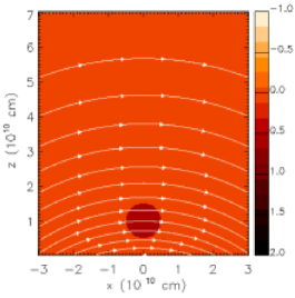
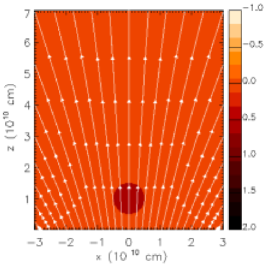
Figure 1: Magnetic field lines and color maps of the density contrast ($\rho/\rho_{0}$) for two different initial configurations of magnetic field: closed field (upper panel, those starting with MC in Table 1) and open field (lower panel, those starting with MO in Table 1).

Other simulations are also performed: we repeat simulations with no magnetic field and with open dipole magnetic field for a spherical cloud (instead of cylindrical), the same as presented in Ciaravella et al. (2001); we make some simulations with a stronger ambient magnetic field (i.e. $\beta\sim 0.25$ at the height of the centre of the initial cloud), a magnetic-field-dominated initial regime. To account for the ejection of both magnetic flux and plasma we replicate the simulation with the open dipole ambient magnetic field for an initially magnetized cylindrical cloud, i.e. an additional magnetic field component inside the cloud along $y$ (i.e. along the axis of the cloud), as shown in Fig. 2. We consider two different values of $B_{y}$: $B_{y}=0.2$ G and $B_{y}=1$ G. With $B_{y}=0.2$ G, the cloud parameters are left unchanged, therefore creating a small overpressure on the ambient medium. With $B_{y}=1$ G, the cloud temperature is set equal to 40,000 K (i.e. much lower than the reference value) to preserve the initial condition of isobaric cloud.

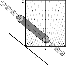
Figure 2: Sketch of the initial configuration of the simulations with an open dipolar ambient magnetic field and an initially magnetized cloud (MOHCL and MOHCH in Table 1). The ambient dipolar magnetic field is shown in the x-z plane (see lower panel of Fig. 1). The additional magnetic field component is set inside the cloud (the long cylinder) along the $y$-direction.

Table 1 lists the relevant simulations presented in this work, identified by the presence or the absence of magnetic field, the magnetic field topology, the value of $\beta$ at the initial height of the cloud centre, the cloud shape, the magnetic field inside the cloud, the presence or absence of thermal conduction, the geometry of the computational domain.

The simulation with open magnetic field and a spherical cloud requires 3-D modeling and we extend the cartesian domain also in the $y$-direction to $y=3\times 10^{10}$ cm. We have performed these simulations on a Cluster Linux EXADRON with 24 Opteron 250 AMD processors and on a IBM SP Cluster with 512 IBM Power5 processors. The 2-D simulations have required $\sim 300$ hours of computational time and the 3-D $\sim 3000$ hours.

3 Results

3.1 Cylindrical cloud

3.1.1 Simulations with no magnetic field

We start the simulation with a cylindrical cloud in the environment without magnetic field as the basic model (case HC, abbreviation for Hydrodynamic model, Cylindrical cloud, in Table 1). As in Ciaravella et al. (2001) the thermal conduction is set to zero in this simulation. Figure 3 shows color maps of the density contrast (ratio of the density to the density of the static atmosphere $\rho/\rho_{0}$) and the temperature at times $t=500$ s, $1500$ s,and $3000$ s, i.e. at two intermediate times and at the final time.

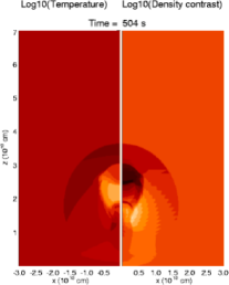
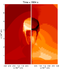
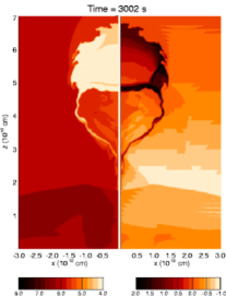
Figure 3: Color maps of temperature (left of each panel) and density contrast, $\rho/\rho_{0}$ (right of each panel) at times $t=500$ s, 1500 s and 3000 s, for the simulation with no magnetic field (and no thermal conduction, HC in Table 1).

The cloud initial velocity is higher than the local sound speed ($c_{S}\sim 200$ km/s) and a shock front soon departs radially from the cloud. While moving upwards, the cloud expands and dynamic instabilities develop at its boundary, changing its shape and forming small scale structures, departing from it. At the final time the cloud has evolved into a cold extended core with two thin tails and has mostly lost memory of its initial circular shape. The core becomes colder and denser during the evolution because of the radiative losses and of the absence of thermal conduction. Since the cloud is stratified, thermal instabilities first occur in the lower (and denser) arc-shaped part, and at the end they involve the whole cloud. Because of the relative motion between the cloud and the atmosphere, Kelvin-Helmholtz and Rayleigh-Taylor instabilities develop in a time-scale (Chen & Lykoudis, 1972):

$$\tau_{KHRT}\approx\frac{\gamma}{\gamma-1}\frac{c_{S}}{g}\sim 10^{3}\leavevmode\nobreak\ s$$ (10)

where $c_{s}$ is the sound speed. The motion of the cloud is mostly ballistic, although it loses part of its mechanical energy (i.e. kinetic plus potential gravitational) in the hydrodynamic interaction with the atmosphere, and at $3000$ s the cloud has practically stopped. To quantify the expansion of the cloud while it moves upwards, we define an expansion factor ($F_{e}$) as the ratio between the maximum width of the cloud (in the $x$-direction) and its initial radius, which can be compared to the factor 3-4 estimated by Ciaravella et al. (2000). At the end the expansion stops and the pressure equilibrium between the cloud and its surroundings is recovered. We obtain $F_{e}\approx 2.9$ at t=3000 s for this simulation.

We do not present here hydrodynamic simulations with the thermal conduction. Ciaravella et al. (2001) showed that if the thermal conduction were not suppressed, the core would mostly evaporate because of heating by the hot surrounding corona and would shrink to a very small cold knot.

3.1.2 Simulations with magnetic field

We now report on results of simulations with an initially cylindrical cloud, with non-zero ambient magnetic field, and with the thermal conduction strongly effective along the magnetic field lines (MCLC, abbreviation for Magnetohydrodynamic model, Closed field, Low $\beta$, Cylindrical cloud, MOLC, MCHC, and MOHC in Table 1).

In the low $\beta$ simulations (MCLC, MOLC) the cloud does not show significant evolution, because the magnetic field is too strong to be perturbed by the moving cloud. The strong magnetic tension does not allow the cloud to move upwards, either. As an example, figure 4 shows the case of the closed dipolar field (MCLC) at $t=500$ s, with $\beta\sim 0.25$ at the initial height of the cloud centre.

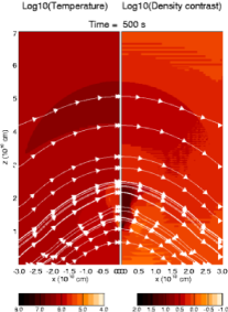
Figure 4: Magnetic field lines and color maps of temperature and density contrast at time $t=500$ s for the simulation with a strong closed magnetic field (MCLC in Table  1). The magnetic field strength is $\approx 2.7$ G at $z\sim 1.5\times 10^{10}$ cm along the x=0 axis (high density field lines) and no field line was drawn in the region where it becomes less than $\sim 1$ G ($z>5\times 10^{10}$ cm).

In the high $\beta$ ambient medium, instead, the cloud moves upwards and expands in the outer corona. Figure 5 shows the evolution of the density contrast and the temperature with color maps at $t=500$ s, 1500 s and 3000 s for the simulation with the closed dipolar field for $\beta\sim 25$ at the initial cloud height.

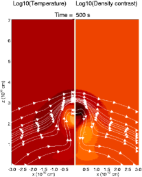
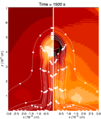
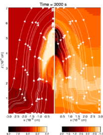
Figure 5: Magnetic field lines and color maps of temperature and density contrast at t=500 s, 1500 s and 3000 s for the simulation with weak closed magnetic field (MCHC in Table 1). For reference, at t=500 s the strength of the magnetic field ranges between $\approx 0.05$ G (in the upper part of the domain where no magnetic field lines are drawn) and $\approx 0.7$ G (just above the cloud where the lines are very dense).

Since the initial cloud velocity (400 km/s) is higher than both the sound speed and the Alfven speed ($v_{A}\sim 10^{7}$ cm/s), a fast MHD shock propagates radially from the cloud. During the evolution no hydrodynamic instability develops because of the suppression by the thermal conduction and the magnetic field. In fact, they are effective on time scales smaller than $\tau_{KHRT}$ (Eq. 10), i.e. of the order of, respectively:

$$\tau_{c}=\frac{21nk_{b}L^{2}}{2k_{0}T^{2.5}}\sim 100\leavevmode\nobreak\ s$$ (11)

$$\tau_{a}=\frac{L}{v_{A}}\sim 100\leavevmode\nobreak\ s$$ (12)

where $k_{0}T^{2.5}=k_{\parallel}$ and for typical coronal density with $k_{0}=9.2\times 10^{-7}$ (c.g.s. units, from Eq.8), $v_{A}$ the Alfven speed, $L$ a characteristic length scale, which we have conservatively taken as half of the cloud radius. The cloud drags the magnetic field lines which gradually envelope the cloud and inhibit thermal exchanges between the cloud and the surrounding medium. The consequent strong thermal insulation leaves the plasma free to cool down to temperatures below $T\approx 10^{5.6}$ K at which it emits the UV lines of interest. The upward motion of the cloud is braked by the restoring forces of the magnetic field; only the upper part of the cloud reaches the UVCS observation height. The cloud expansion is limited by the confining effect of the magnetic field, which becomes up to 5 times stronger just outside the cloud ($\beta\sim 0.1$) than inside it. At the end, the expansion factor of the cloud is $F_{e}\approx 2.1$ at $t\sim 3000$ s (i.e. $\sim 70\%$ of the reference case).

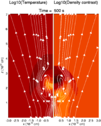
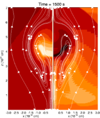
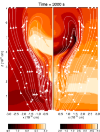
Figure 6: Magnetic field lines and color maps of temperature and density contrast at t=500 s, 1500 s and 3000 s for the simulation with weak open magnetic field (MOHC in Table 1). The strength of the magnetic field ranges from $\approx 0.03$ G to $\approx 0.5$ G.

The cloud travels much longer distances when it moves in an open ambient magnetic field. Figure 6 shows the evolution of the density contrast and of the temperature at $t=500$ s, $1500$ s and $3000$ s for the related simulation. Again, a fast MHD shock propagates upward radially from the cloud and no hydrodynamic instability develops. At variance with the closed field case, in the open field the cloud moves ballistically to the outer corona. The cloud is thermally insulated laterally, because the initial field direction is mostly maintained during the evolution. In the upper corona, the magnetic field is weak and, therefore, perturbed by the rising cloud (at $t>2000$ s). A strong magnetic field horizontal component develops ahead of the cloud and inhibits thermal conduction with the region above the cloud. As the magnetic field in the cloud is frozen and the cloud moves fast with respect to the Alfvén scale times, it drags the magnetic field lines, and inversely-directed downward magnetic field components and current sheets are produced near the cloud. The open magnetic field naturally favours the cloud expansion and, in fact, the final expansion factor is $F_{e}\approx 3.9$ at $t\sim 3000$ s (i.e. $\sim 35\%$ more than the reference case).

3.2 Spherical cloud

We now present results for the case of a spherical cloud. We compare the null-field evolution (the one presented with the highest detail in Ciaravella et al. (2001), HS in Table 1) with the evolution of the cloud in the weak open dipole field ($\beta\sim 25$ at the initial cloud height, MOHS in Table 1), performed with a fully 3-D simulation. Figure 7 shows the density contrast for both the simulations.

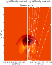
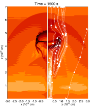
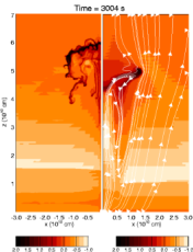
Figure 7: Magnetic field lines and color maps (on the section across the cloud axis) of density contrast at t=500 s, 1500 s and 3000 s for the simulations of a spherical cloud without magnetic field (left of each panel, HS in Table 1) and with a weak open magnetic field (right of each panel, MOHS in Table 1). The strength of the magnetic field ranges from $\approx 0.03$ G to $\approx 0.5$ G.

In the HD simulation (HS), the cloud evolves into a thin dense shell-like structure, with very irregular boundaries, due to the hydrodynamic instabilities, that can develop in the absence of thermal conduction. At the end of the evolution, the expansion factor of the cloud is $F_{e}\approx 2.7$ at $t\sim 3000$ s. Since the volume expansion of the spherical cloud scales as $r^{3}$, the corresponding projected expansion is less significant than the projected expansion of the cylindrical cloud, whose volume expansion scales as $r^{2}$. In the MHD simulation (MOHS), the more effective expansion makes the cloud apparently less conspicuous than in the case of the cylindrical cloud (Fig.6). The expansion factor is $F_{e}=2.8$ at $t\sim 3000$ s, $\sim 4\%$ more than the HD case, and $\sim 70\%$ of the expansion of the cylindrical cloud (MOHC, see Section 3.1.2).

3.3 Magnetized cloud

As mentioned in Section 2, we consider two simulations of magnetized clouds, one with a weak (0.2 G) internal $B_{y}$-component (i.e. along the axis of the cylindrical cloud, as sketched in Fig. 2, MOHCL (abbreviation for Magnetohydrodynamic model, Open field, High $\beta$, Cylindrical cloud, Low internal magnetic field) in Table 1, the other with a strong (1 G) $B_{y}$-component (MOHCH) in Table 1. We will not comment much on the latter case, because we found that the whole cloud remains very cool all over the computed evolution, much cooler than the temperature of formation of the relevant UVCS lines. This case therefore seems to be unrealistic.

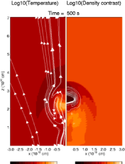
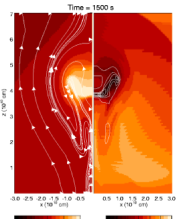
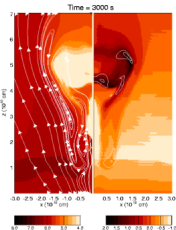
Figure 8: Magnetic field lines (x-z plane, left of each panel), color maps of temperature (left) and density contrast (right), and contours of the magnetic field $y$-component (right) at time t=500 s, 1500 s and 3000 s for the simulation with a weak open ambient field and a weak magnetic field $y$-component inside the cloud (MOHCL in Table 1). The contours of $B_{y}$ are spaced by $0.02$ G to a maximum of 0.2 G. The strength of the magnetic field on the left of the panels ranges from $\approx 0.03$ G to $\approx 0.5$ G.

Figure 8 shows magnetic field, density contrast and temperature distributions over the cloud cross-section for the simulation with the weaker magnetic field component inside the cloud (MOHCL). The global evolution does not change significantly with respect to the case of no internal magnetic field (MOHC, Section 3.1.2), and the morphology of the cloud evolves similarly to that of Figure 6. Therefore, the presence of an internal magnetic field component does not influence much the evolution of the cloud, in spite of the initial cloud overpressure. The latter is only a small cloud rapidly absorbed by the corona in $\tau\approx L/c_{S}\sim 250s$, where $L=5\times 10^{9}$ cm is the cloud size. The contours on the right side of the panels of Fig. 8 show that the $B_{y}$ component initially set up inside the cloud becomes weaker and weaker as the cloud moves upwards and expands.

The cloud thermal insulation is very good in this simulation, as indicated by the growing cold core, even more extended than in the other simulations. The magnetic field component along the axis of a cylinder infinitely extending horizontally further inhibit thermal exchanges with the surrounding corona. In a more realistic configuration of an elongated cloud with an internal magnetic field which bends downwards and eventually connects to the photosphere (e.g. a flux rope), some heat would be conducted to the footpoints, similar to the 1-D conduction case described in Ciaravella et al. (2001). We estimate that the cloud would thermalize in $\tau_{c}\sim 1000$ s (see Eq.11), if the lenght scale of the cloud is the same as its height, say $h\sim 10^{10}$ cm, above the photosphere. The cloud expansion factor for this case of magnetized cloud is $F_{e}\approx 3.6$ at $t\sim 3000$ s.

4 Discussion and conclusions

This work is devoted to studying the role of the magnetic fields in the evolution of a fragment of a CME core traveling upwards in the high solar corona. We address the late stage evolution of the cloud, in which it travels in a weakly magnetized atmosphere ($\beta\ga 1$). Our simulations show that the evolution in the late stage could be described better than in the early stage. In particular, we focus on the thermal insulation of the cloud and on its degree of expansion; both aspects were not well explained with a purely hydrodynamic model (Ciaravella et al., 2001). In the simulations presented here, we basically consider infinitely long cylindrical clouds, and we first investigate which configuration (i.e. strength and topology) of the ambient magnetic field could favor better the thermal insulation and the expansion of the cloud simultaneously.

Before investigating the cloud enclosed by magnetic fields, we screen out those ambient magnetic field configurations which strongly brake the upward motion of the cloud, i.e. provide magnetic confinement. Since the plasma is frozen to the field, the cloud moving upward drags the ambient magnetic field. The strong magnetic tension then acts against the cloud expansion and motion. Our simulations show that the cloud is strongly braked in an atmosphere with $\beta<1$ (see Fig.4), and is much easier to move with $\beta>1$.

In a weak ambient magnetic field ($\beta>1$), the cloud expands while it moves. The evolution naturally leads to the strong thermal insulation of the cloud because it is fast enough to drag the magnetic field so as to be “wrapped” by it, and to be thermally insulated from the surroundings. For weak magnetic fields, the closed field topology yields the best thermal insulation because the magnetic field perfectly envelops the rising cloud. However, for the same reason, it limits the cloud expansion and motion.

The observation supports the result of the linear expansion of a factor of 3-4 (Ciaravella et al. 2000). In the circumstances of the cylindrical clouds, we find an expansion factor $F_{e}\approx 2.1$ for the closed magnetic field simulation, $F_{e}=3.9$ for the open magnetic field and an intermediate value $F_{e}\approx 2.9$ for the basic hydrodynamic case. Thus, the open field favours the cloud expansion, while the closed field does not. The expansion of the cloud nearly stops at the end of the simulations because the pressure equilibrium is reestablished between the cloud and the surroundings, and, as Riley & Crooker (2004) pointed out, the magnetic tension is not important as restoring force.

We find similar results and an expansion factor $F_{e}=3.6$ for the simulation of a cylindrical cloud which carries an initial moderate magnetic field component along its axis. A strong internal field does not appear realistic in our conditions because it would imply an extremely cool cloud all along its evolution, in contrast with observations. The effect of the internal magnetic field component is to further funnel heat transport and therefore reduce thermal exchanges with the surroundings. However, we should expect thermal exchanges at the extremes of a more realistic finite cylindrical cloud.

We conclude that the open field topology is most conducive to both the thermal insulation and a good degree of expansion, and may therefore be the best match to observations. This is true regardless if we consider a purely plasma cloud or a cloud accounting also for the ejection of magnetic flux. Several CME models already considered an open ambient magnetic field in the outer corona in order to take into account a steady solar wind flow (Manchester et al., 2004; Chané et al., 2005; Lugaz et al., 2005). Moreover, Cargill & Schmidt (2002) considered the model of an emerging flux rope evolving in a open magnetic field.

Our work shows that the cloud mass and shape are also important. The expansion factor of an initially spherical cloud increases by $\sim 4\%$ more in an ambient open field than with no field. Instead, for an elongated cloud the increase is of $\sim 35\%$. Thus, although the open field induces a larger expansion regardless the cloud geometry, this effect is more significant for an elongated cloud than for a spherical one. This is in agreement with many models that consider a filament eruption or a emerging flux rope as the possible initiation or triggering of a CME (Forbes & Isenberg, 1991; Linker et al., 2003; Moore et al., 2001; Török & Kliem, 2005).

We finally remark that we assume conditions of ideal MHD (except for numerical diffusivity that gives an effective magnetic Reynolds number $R_{m}\apprge 50$). It will be interesting to investigate in the future the role of the magnetic diffusion and joule heating, which may be important locally in some areas, in which the magnetic field is found to be enhanced during the propagation of the cloud.