Modeling the Stellar Populations in the Canis Major Over-Density: the Relation Between the Old and Young Populations

Abstract

We analyze the stellar populations of the Canis Major stellar over-density, using quantitative color-magnitude diagram (CMD) fitting techniques. The analysis is based on photometry obtained with the Wide Field Imager at the 2.2m telescope at La Silla for several fields near the probable center of the over-density. A modified version of the MATCH software package was applied to fit the observed CMDs, enabling us to constrain the properties of the old and young stellar populations that appear to be present. For the old population we find [Fe/H]$\sim$-1.0, a distance of $\sim$7.5 kpc and a line-of-sight depth $\sigma_{los}$ of 1.5$\pm$0.2 kpc and a characteristic age range of 3-6 Gyrs. However, the spread in ages and the possible presence of a $\sim$10 Gyr old population cannot be constrained. The young main-sequence is found to have an age spread; ages must range from a few hundred Myr to 2 Gyr. Because of the degeneracy between distance and metallicity in CMDs the estimates of these parameters are strongly correlated and two scenarios are consistent with the data: if the young stars have a similar metallicity to the old stars, they are equidistant and therefore co-spatial with the old stars; if the young stars have close to solar metallicity they are more distant ($\sim$9 kpc). The relatively low metallicity of the old main-sequence favors the interpretation that CMa is the remnant of an accreted dwarf galaxy. Spectroscopic metallicity measurements are needed to determine whether the young main-sequence is co-spatial.

1. Introduction

A few years ago Martin et al. (2004a) discovered an apparent over-density of M-giant stars in the direction of the constellation Canis Major (CMa), using 2MASS data. They also reported that the structure was surrounded by a number of globular and open clusters. Combined with the fact that it is located at low galactic latitudes, just below the plane of the disk of the Milky Way, led them to conclude that it may well be the (remnant of a) disrupted dwarf galaxy that could have spawned the so-called Monoceros stellar stream. That stellar stream had been discovered some years prior (Newberg et al., 2002; Yanny et al., 2003) and seems to surround the Galaxy completely at very low galactic latitudes. Numerical simulations show that such a system can be explained by an in-plane accretion event (e.g. Peñarrubia et al., 2005). Subsequent deep photometric observations (Martinez-Delgado et al., 2005; Bellazzini et al., 2004), kinematic studies (Martin et al., 2004b, 2005) and analysis of 2MASS data (Bellazzini et al., 2006) are in accord with this scenario. The optical photometry also revealed the presence of a young main sequence population of stars potentially at the same distance. The initial analysis of a new wide-field survey of the CMa region revealed that the projected distribution of the young stars is qualitatively similar to the older population (Butler et al., 2006).

However, other explanations for the observed stellar over-density have been offered. Momany et al. (2004) and Momany et al. (2006) argued that the observed stellar over-densities towards CMa reflect the warp and flare of the outer disk. Carraro et al. (2005) and Moitinho et al. (2006) argued that the intrinsic substructure of the disk such as spiral arms can explain the observations if they are not in the plane of the disk. In this picture the young main sequence (YMS) population is related to the outer Cygnus spiral arm, while the older main sequence (OMS) feature is caused by disk stars in the inter-arm region between the Cygnus and Perseus spiral arms. In the latter scenario the OMS and YMS populations would be located at different distances and not actually co-spatial.

The generic problem with the interpretation of the observed features is that since they are lying so close to the plane of the disk it is a priori not clear if they are intrinsic to the disk or have an outside origin.

We are performing a large photometric survey of the CMa over-density using the Wide Field Imager (WFI) on the ESO/MPG 2.2m telescope at La Silla. Based on a relatively straightforward analysis of the color-magnitude diagrams (CMDs) we have estimated the line-of-sight (l.o.s.) depth of the over-density and its spatial extent in (Butler et al., 2006, B06). The picture that emerged is that of an old stellar over-density that is highly elongated in Galactic longitude with a projected aspect ratio of $\gtrsim$5:1, consistent with recent 2MASS analyses (Bellazzini et al., 2006; Rocha-Pinto et al., 2006). The YMS stars show qualitatively a similar projected distribution but are markedly more localized, both in galactic longitude and latitude with a maximum near ($l$,$b$)$\sim$(240°,-7°). For the extent of the over-density along the l.o.s., $\sigma_{los}$, B06 found upper limits of 1.8 and 1.5 kpc for the OMS and YMS respectively, assuming an average distance of 7.5 kpc for both populations.

The main aim of this paper is to extract more information from the photometry by applying more sophisticated CMD-fitting methods. In particular we are interested whether the OMS and YMS over-density populations seen towards CMa can be co-spatial, based on our optical photometry. We also constrain the metallicity of the YMS stars, which has so far not been constrained. To do this we apply CMD-fitting techniques to a small selection of fields towards the likely maximum of the CMa over-density from our large photometric survey.

Fitting of CMDs with model stellar populations enables use of the full distribution of stars within a CMD. Methods to obtain detailed information on the star formation and chemical enrichment history of composite stellar systems have been proven to be very successful (see e.g. Gallart et al., 1996; Tolstoy & Saha, 1996; Aparicio, Gallart & Bertelli, 1997; Dolphin, 1997; Holtzman et al., 1999; Olsen, 1999; Hernandez, Gilmore & Valls-Gabaud, 2000; Harris & Zaritsky, 2001; Dolphin, 2002). For the analysis in this paper a modified version of the software package MATCH (e.g. Dolphin, 1997, 2002) is used. It uses maximum-likelihood techniques to find the linear combination of single-component stellar population models that best fits an observed Hess diagram (stellar density as function of color and magnitude).

The remainder of the paper is organized as follows: Section 2 describes the data and methods used. In Sections 3 and 4 the results of our fits are presented and their implications are discussed in section 5. Finally, section 6 presents our conclusions.

2. Data and methods

Figure 1.— Completeness of the stellar photometry for the four fields (see section 2.1) used in the current analysis, determined from the artificial star tests. Solid lines are for B band and dashed lines for R band. The limiting magnitudes we use for our CMD fits, B=22 and R=21, are indicated with vertical lines.

This analysis is based on deep B,R photometry obtained with the Wide Field Imager (WFI) at the ESO/MPG 2.2m telescope at La Silla. These data are part of an extensive survey of the Canis Major region, presented in B06. Because of the amount of data involved, the data reduction used for the complete survey as described by B06 is fully automated. For the analysis in this paper, accurate calibration of the photometry is critical. We use the same reduced image data, which are overscan, bias, flat-field and astrometrically corrected using a pre-reduction pipeline (Schirmer et al., 2003), but individually re-calibrate the magnitudes for our CMa fields to ensure the best possible photometric accuracy.

Standard star fields taken on the same night (2004 December 9) as three of the CMa fields were used to determine the zero-points, color terms and airmass correction factors. The values found were very close to the ones provided by ESO. Based on these standard star measurements we estimate the color calibration accuracy to be 5%. Object detection was performed using SExtractor Bertin & Arnouts (1996), after which PSF-fitting photometry was done with the IRAF task DAOPHOT/ALLSTAR. Fake star tests were also done by adding artificial stars to the images using an empirical PSF measured from stars in the image and subsequently running the same detection and photometry routines. Six sets of 1000 artificial stars spread over a wide magnitude range (15-24 for B-band, 14-23 for R-band) were used for each image, giving 6000 fake stars per image. For the analysis presented here we will only go down to magnitudes of 22 in B and 21 in R. Figure 1 shows that the data are complete to $\sim$80% complete or better at these limits. Typical photometric errors at these magnitudes are 0.05 mag and better at brighter magnitudes.

The CMD fitting software needs artificial star files with large numbers of stars spread over the whole magnitude and color range used. B-band and R-band artificial star data are randomly combined within a color range of -1.0$<$B-R$<$3.0 to create lists of more than 80,000 entries for each field.

2.1. Fields used and extinction

Figure 2.— Locations of the fields used for the current analysis, where squares indicate the CMa fields and triangles the control fields. The dotted line indicates the Galactic plane at $b$=0°and the contours correspond to constant differential extinction values of $E(B-V)=1.0$ and 0.4 mag, based on the dust opacity maps by Schlegel, Finkbeiner & Davis (1998).

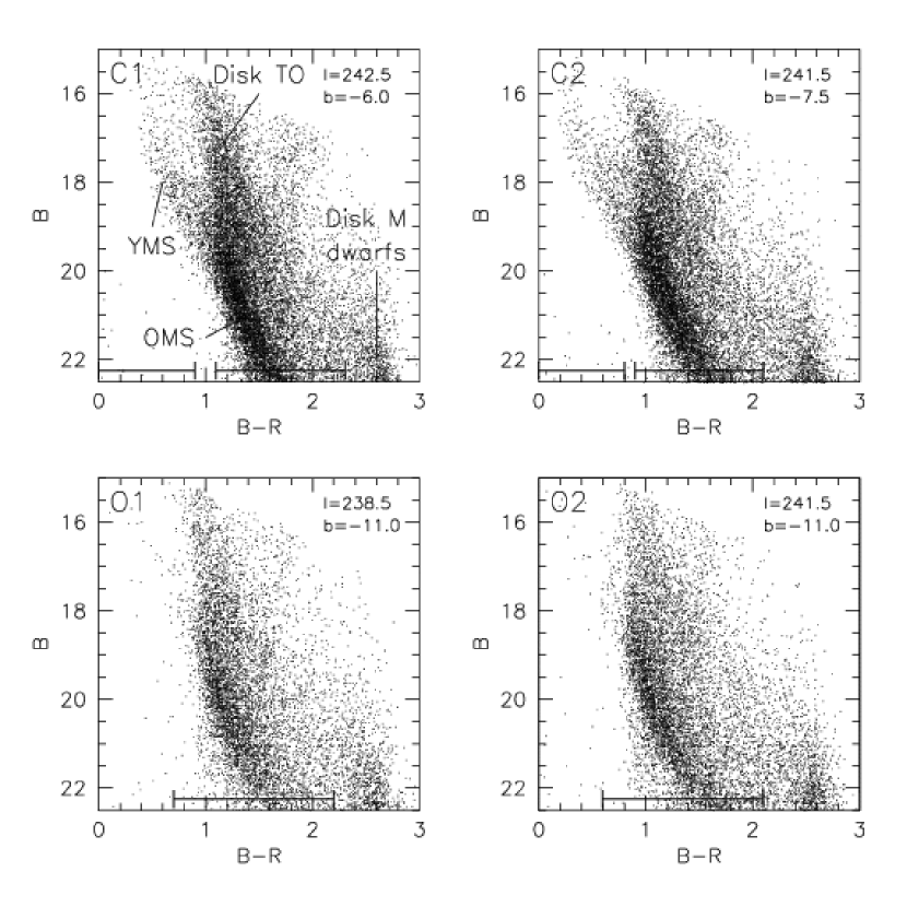
Figure 3.— Color-magnitude diagrams (CMD) of the CMa fields selected for the present analysis. The upper panels show the central fields C1 (left) and C2 (right) and the lower panels the outer fields O1 (left) and O2 (right), respectively. Each field is $\sim$0.2 sq.deg. in area. At the bottom of each CMD the color ranges used later for the separate fits to the young and old stars are indicated. In the upper left panel the obvious features are labeled. A near-vertical swath of predominantly thin and thick disk main-sequence turn-off stars is present in all fields, labeled with “Disk TO”. At the bottom right of the CMD, “Disk M dwarfs” indicates the location of a concentration of thin and thick disk M dwarfs. The young main sequence (YMS) and old main sequence (OMS) of CMa are also labeled.

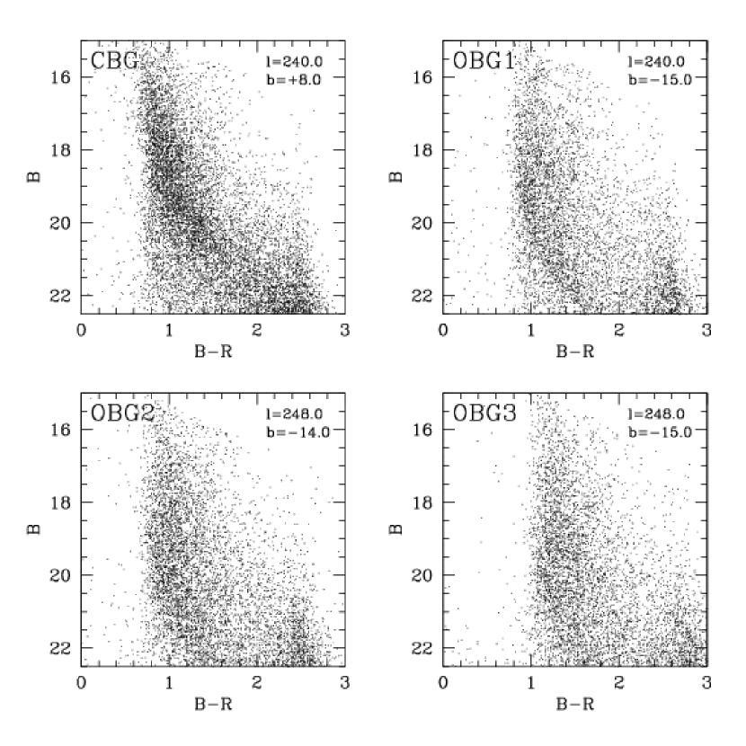
Figure 4.— Color-magnitude diagrams of the control fields selected for the current analysis. In absence of CMa stars, the halo, thick disk and thin disk features (see Figure 3) are clearly seen.

Table 1Overview of used fields

Field	$l$ (°)	$b$ (°)	$<A_{V,SFD}>$ (mag)
CMa Fields
C1	242.5	-6.0	1.13 [0.85,1.28]
C2	241.5	-7.5	0.76 [0.63,1.03]
O1	238.5	-11.0	0.54 [0.49,0.64]
O2	241.5	-11.0	0.42 [0.38,0.49]
Control Fields
CBG	240.0	8.0	0.40 [0.35,0.42]
OBG1	240.0	-15.0	0.32 [0.30,0.39]
OBG2	248.0	-14.0	0.71 [0.61,0.83]
OBG3	248.0	-15.0	0.61 [0.52,0.82]

Note. — C1, C2, O1 and O2 are the CMa fields that are the subject of the present analysis. CBG is the control field used for fields C1 and C2; OBG1, OBG2 and OBG3 are used to construct control field CMDs for O1 and O2. Column four gives the median extinction towards each field, with in brackets the maximum and minimum values (Schlegel, Finkbeiner & Davis, 1998).

As shown by B06, our imaging survey traces the CMa over-density over a large area ($\sim$80°$\times$20°), but for this first CMD analysis we limit ourselves to a small number of fields. To maximize signal-to-noise (the number of CMa stars vs. the number of fore- and background stars) and since the YMS is spatially less extended than the OMS (B06), we chose to use fields near the presumed center of the over-density at ($l$,$b$)=(240°,-7°). In order to see whether the properties of the OMS change with galactic latitude we also want to study some fields farther away from the plane. To be able to check for internal errors we choose to use 2 fields near the presumed center of CMa and 2 fields that are at a latitude of $b\simeq-11$°. Since the CMa over-density is located at very low galactic latitudes, just south of the plane of the disk, the number of fore- and background disk stars is very high. This necessitates the use of control fields in our analysis, and appropriate fields need to be selected for this purpose as well.

Because of the location of the CMa over-density close to the Galactic plane, the extinction in the observed fields is high and increasing along the l.o.s.. Furthermore, the extinction correction in B06 has shown that the extinction estimates from Schlegel, Finkbeiner & Davis (1998) and Bonifacio et al. (2000) in some cases seem to overestimate and in others to underestimate the actual extinction. This is problematic for our analysis since an unknown extinction introduces large uncertainties in the CMD-fitting analysis due to the degeneracies between extinction, age, metallicity and distance. To minimize these uncertainties we select fields with relatively low (but certainly still significant) extinction for our analysis.

Table 1 lists the coordinates and average extinction values of the selected fields, where C1 and C2 correspond to the “central” fields, i.e. near the CMa center ($b\approx$-7°), and O1 and O2 to the “outer” fields ($b=$-11°). Also listed are the fields that will be used to construct control fields. For fields C1 and C2 a field at similar longitude and similar latitude north of the disk plane will be used for control field; this field shows no significant contribution of CMa stars and is listed in Table 1 as CBG. Since fields farther away from the plane contain much less stars, we combine CMDs from three fields at low latitude to construct control fields for the fields O1 and O2. These three control fields (OBG1, OBG2 and OBG3 in Table 1) are selected to contain no or very few CMa stars and to have similar extinction as fields O1 and O2. The locations of the selected fields are plotted in Figure 2, together with contours indicating the extinction in the Galactic plane. In Figure 3 the CMDs of the CMa target fields are shown, and in Figure 4 the CMDs of the control fields.

2.2. CMD fitting methods

As mentioned in Section 1, quantitative and algorithmic CMD (or Hess diagram) fitting methods have proven themselves and several software packages have been developed for this aim (Gallart et al., 1996; Tolstoy & Saha, 1996; Aparicio, Gallart & Bertelli, 1997; Dolphin, 1997; Holtzman et al., 1999; Olsen, 1999; Hernandez, Gilmore & Valls-Gabaud, 2000; Harris & Zaritsky, 2001). The software package we use is MATCH, which was written and successfully used for the CMD analysis of globular clusters and dwarf galaxies (Dolphin, 2002). The software works by converting the observed CMD into a Hess diagram and comparing that with Hess diagrams of model populations. A Hess diagram is a two-dimensional histogram of stellar density as function of color and magnitude. Theoretical isochrones (Girardi et al., 2002, in the case of MATCH) are convolved with a model of the photometric accuracy and completeness, obtained from the artificial star test data, to create the model Hess diagrams. The use of Hess diagrams enables a pixel-by-pixel comparison and a maximum-likelihood technique is used to find the best-fitting linear combination of models. To account for contamination by fore- and background stars, a control field CMD can be provided. MATCH will then use the control field Hess diagram as an extra ‘model population’. The resulting output will be the best-fitting linear combination of population models plus the control field. Previously MATCH was used in a mode where extinction and distance are fixed and the best-fitting combination of models with different age and metallicity are found. For the application described in this paper, we have used MATCH in somewhat different modes, namely one where distance is a free parameter and one where only simple, single component models are fit to the data and compared based on their goodness-of-fit.

MATCH was originally developed for systems where all stars can be assumed to be at the same distance, i.e. external galaxies. In the case of the CMa over-density this approximation does not apply, as it is relatively nearby and has a significant extent along the l.o.s. (e.g. Martinez-Delgado et al., 2005; Butler et al., 2006). Moreover, it is possible that the OMS and YMS populations are only co-spatial in projection and actually at different distances (Moitinho et al., 2006). Thus, there are two effects we need to cope with, namely distance spread of populations and distance offsets between populations. Accounting for a distance spread can be done in a straightforward way by manipulating the photometric error model; adding random offsets with a normal distribution to the recovered magnitudes of the artificial stars will smooth the model Hess diagram along the magnitude axis with the same $\sigma$. To fit populations at different distances simultaneously we have implemented a new way in which to run MATCH that keeps the same number of free parameters, or parameter dimensions, to be explored. In the standard mode, the distance is fixed, while age and metallicity are independent variables. Here, the distance becomes a free parameter, but age and metallicity are being limited via a specified age metallicity relation (AMR). For any given AMR there is only one “population parameter”, e.g. age with a certain metallicity linked to each age bin. Of course, different AMRs can be explored, ultimately permitting a wide range of age-metallicity relations. In general, AMRs should be chosen that are appropriate for the specific application, based on expected or known metallicity evolution. For example, for the study of structures in the Galactic thin disk one would consider a different AMR than for the study of a metal-poor dwarf galaxy. However, within this new mode of running MATCH the choice of AMR is very flexible and a flat AMR (no dependence of metallicity on age) or even an AMR where metallicity decreases with time is possible. In section 4 of this paper we will use two different AMRs to constrain how the assumed metallicity influences the distances found through CMD-fitting.

Because of the large contamination of the CMa CMDs with fore- and background stars, a feature like the red giant branch (RGB) is observed at very low contrast. The main sequence (MS) is the only feature that is observed with high contrast and significance, and MATCH can fit the location of the MS and the MS turn-off (MSTO), as well as the density of stars along the MS. To constrain the basic parameters of CMa – distance, age range, and average metallicity – we first use MATCH in a single component (SC) fitting mode; in this mode, template stellar population models are created that consist of a single component with fixed distance, foreground extinction, age range and metallicity range. Such a SC template is fit to the data together with a control field. Since the template consists of a single component, the only free parameters during the fit are the absolute scaling of (i.e. the number of stars in) the template and the control field. For each template (i.e. for each combination of distance, foreground extinction, age range and metallicity range), taken by itself, a value of the goodness-of-fit is obtained. Based on the goodness-of-fit values we can then find the best-fitting template and thus constrain the overall properties of the CMa YMS and OMS populations. A paper describing the application of these new modes of application of MATCH, including tests and simulations is in preparation (J.T.A. de Jong et al. 2007, in preparation).

It should be noted that the results of CMD fits depend on the assumed set of theoretical stellar evolution models. When MATCH was written, the only set of isochrones with full age and metallicity coverage available was provided by Girardi et al. (2002). Since MATCH only uses one set of isochrones, this adds a further source of uncertainty to our fit results.

From the CMDs presented here and in B06, the OMS and YMS seem to be two distinct populations. In Section 3 we first study the populations separately using SC template fits. To better study the relation between these two populations, we also fit them simultaneously using the new capability of MATCH to solve for distance. Section 4 describes the results of these distance distribution fits to the complete CMa CMDs.

3. Single component fits to the CMDs

Table 2Single Component Fitting Results

Parameter	C1 OMS	C2 OMS	O1 OMS	O2 OMS	C1 YMS	C2 YMS
$B-R$ range (mag)	[1.1,2.3]	[0.9,2.1]	[0.7,2.2]	[0.6,2.1]	[0.0,0.9]	[0.0,0.8]
AV,fg (mag)	1.2$\pm$0.1	0.9$\pm$0.2	0.7$\pm$0.2	0.5$\pm$0.2	0.9$\pm$0.1	0.6$\pm$0.1
Agell (log(yr))	9.5$\pm$0.1	9.4$\pm$0.1	9.5$\pm$0.1	9.5$\pm$0.1	8.4$\pm$0.3	8.4$\pm$0.0
Ageul (log(yr))	9.7$\pm$0.1	9.7$\pm$0.1	9.7$\pm$0.1	9.7$\pm$0.1	9.3$\pm$0.0	9.3$\pm$0.0
$[Fe/H]$ (dex)	-1.0$\pm$0.2	-1.1$\pm$0.3	-0.6$\pm$0.3	-0.6$\pm$0.3	-0.4$\pm$0.2	-0.3$\pm$0.2
m-M (mag)	14.35$\pm$0.08	14.45$\pm$0.09	14.2$\pm$0.2	14.3$\pm$0.2	14.8$\pm$0.3	14.9$\pm$0.2
$\sigma_{los}$ (mag)	0.44$\pm$0.06	0.39$\pm$0.05	0.44$\pm$0.06	0.39$\pm$0.07	0.44$\pm$0.07	0.31$\pm$0.07

Note. — Age_ll and Age_ul stand for the lower limit and upper limit of the best-fit age range. The $B-R$ range corresponds to the color range in the observed Hess-diagram that is used in the SC fits to single out either the OMS or the YMS. It differs from field to field mainly because of differences in extinction. There are no YMS results for fields O1 and O2, as in these fields the YMS is absent. The errors given here are the standard deviations in the values given by all acceptable fits to the data.

3.1. Fit setup

The OMS is present in all four CMa fields, but with highest signal-to-noise (S/N) in the fields near the presumed density maximum of CMa at ($l$,$b$)$\simeq$(240°,-7°). To only fit the OMS we use color cuts to isolate the regions of the CMDs where the OMS population is located. The color range used for each field is listed in Table 2 and indicated in Figure 3. For C1 and C2 we use the CBG control field as background, where small photometric offsets are applied to CBG to better match the extinction of each field. Since the exact extinctions are uncertain this is done “by eye”, using the locations of the blue edge of disk MSTO stars and the clump of M dwarfs as a guide. For O1 and O2 we create background CMDs by applying separate offsets to control fields OBG1, OBG2 and OBG3 and then combining them. To test how sensitive our results are to the exact control field match, tests were performed where the photometric offsets of the control fields were varied by 0.05 magnitudes in color and 0.15 magnitudes in brightness. This influences the recovered metallicities as presented later on by at most $\sim$0.1 dex, the foreground extinction by up to 0.1 magnitudes, and the distance modulus also by at most 0.1 magnitudes; the age estimates are not significantly affected.

A range of SC models is generated to be compared with the observed Hess-diagrams and each has a specific age range, metallicity, distance modulus, l.o.s. spread, and foreground extinction as detailed below. In all our models we assume a realistic binary fraction for main-sequence disk stars of 0.6 (Duquennoy & Mayor, 1991; Kroupa et al., 1993). For fitting the OMS we use 14 metallicity bins varying from [Fe/H]=-2.05 to -0.1 in steps of 0.15 dex and in all cases there is uniform metallicity spread of 0.2 dex. Distance moduli sampled run from 13.5 to 15.5 mag in steps of 0.1 mag, a range including the distance measured previously for the OMS Martin et al. (2004b); Martinez-Delgado et al. (2005); Bellazzini et al. (2006) and the distance to the outer spiral arm, possibly the distance of the YMS. Extinctions vary from $A_{V}$=0.5 to 1.4 mag in steps of 0.1 mag for C1 and C2 and from $A_{V}$=0.2 to 1.0 mag in steps of 0.1 mag for O1 and O2. Age bins probed vary both in average age as well as in age spread and star formation is assumed to be constant during the entire width of an age bin; we use seven narrow bins with ages in log(years) of 9.4 to 9.5, 9.5 to 9.6, 9.6 to 9.7, 9.7 to 9.8, 9.8 to 9.9, 9.9 to 10.0 and 10.0 to 10.1; seven broader age bins run from 9.5 to 9.7, 9.7 to 9.9, 9.9 to 10.1, 9.5 to 9.8, 9.8 to 10.1, 9.3 to 9.7, and 9.7 to 10.1, respectively. This total of 14 age bins covers ages from $\sim$2 Gyr to $\sim$12.5 Gyr, while the narrowest reflects and age spread of only 650 Myr and the widest presumes ongoing star formation for 7.5 Gyrs. To probe the l.o.s. depth of the OMS, each model is also broadened in magnitude with a Gaussian kernel of a certain $\sigma_{los}$. We probe values 0.2 to 0.6 mag in steps of 0.05 mag; at a distance modulus of 14.5, a step of 0.05 magnitudes corresponds to $\sim$0.18 kpc.

The YMS is only present in the central fields C1 and C2. For fitting we use the part of the CMDs blue-ward of $B-R\sim 1$ where this is the predominant population, see Table 2 and Figure 3 for the exact color ranges. Again we probe the metallicity range [Fe/H]=-2.05 to -0.1 in steps of 0.15 dex and with a metallicity spread of 0.2 dex. Distance moduli again range from 13.5 to 15.5 mag with a 0.1 magnitude resolution. Extinctions vary from $A_{V}$=0.5 to 1.4 mag in steps of 0.1 mag. Twelve age ranges are probed, namely seven narrow ones from 6.6 to 7.05, 7.05 to 7.5, 7.5 to 7.95, 7.95 to 8.4, 8.4 to 8.85, 8.85 to 9.3, and 9.3 to 9.75, and five broader ones from 6.6 to 7.5, 7.5 to 8.4, 8.4 to 9.3, 6.6 to 8.4, and 7.5 to 9.3, all in log(years). Again we try different l.o.s. depths in steps of 0.05 magnitudes. There is little contamination by fore- and background stars for $B-R<1$ and especially for field C2 the YMS stars are easily separated from the contaminants. In the C1 CMD the YMS stars do overlap slightly with young, blue thin disk stars and to take this into account a control CMD was created based on the CBG control field.

The quality of each fit is determined using the maximum-likelihood technique described in Dolphin (2002). This statistic is meant to measure how likely it is that the observed distribution of stars would result from a random drawing from the fitted model. In the current analysis, we know that our fits will not be perfect since the control field is not perfect and the SC models we use will not be a perfect representation of the CMa stellar populations. We therefore need a relative way of comparing the goodness-of-fit of each model. Monte Carlo simulations using random drawings from the models and bootstrap tests where new CMDs are created by drawing at random individual stars from the target CMD are performed for this purpose. From the results the expected 1 $\sigma$ spread in the goodness-of-fit for each field is determined. We then assume that all model fits that have a goodness-of-fit value within 1 $\sigma$ of the best fit are statistically good fits to the data.

To illustrate the SC fitting procedure, we show in Figure 5 the observed Hess diagram, the synthetic Hess diagram (background + CMa model) of the best fit, the residuals between the observed and synthetic Hess diagrams and the residual significance for the OMS in field C2 as an example. It shows that the observed OMS feature can be modeled well with a relatively simple SC model. Figure 6 shows the same for the YMS in field C2.

3.2. Results

Table 2 presents the CMa properties we derive for the OMS and YMS in each field using the above methods. The quoted values are the unweighted averages of the values of all fits that lie within 1 $\sigma$ of the best fit, where $\sigma$ was determined as described above. The quoted errors are the standard deviations in the values. Since there are degeneracies between the different parameters, the actual range of, for example, ages that gives an acceptable fit can actually be larger than is suggested from these quoted errors, but only with a certain combination of values for the other parameters. The standard deviations given here are merely a measure of the scatter in the parameter values for all acceptable fits. Of the $\sim$200,000 SCs that were fit to each OMS, around 100 (0.05%) gave acceptable fits (within 1$\sigma$ from the best fit) for fields C1 and C2 and around 1000 (0.5%) for fields O1 and O2, owing to the smaller significance of the OMS feature in the latter two fields. To each YMS $\sim$100,000 SCs were fit, from which around 100 (0.1%) were within 1$\sigma$ from the best fit.

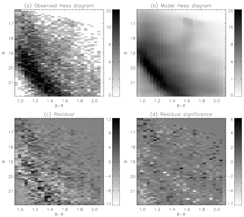
Figure 5.— SC fit to the OMS in field C2. (a) Observed Hess diagram; the grey level gives the number of stars in each color-magnitude box with dark corresponding to high density. (b) Modeled Hess diagram, consisting of the background CBG and the best-fitting SC model. (c) Fit residuals, where light color corresponds to bins where the data is high and dark to bins where the model is high. (d) Significance of the fit residuals; this is a function of the discrepancy between data and model and the total number of stars in the bin. Important is that even when using a relatively simple SC model there are no significant systematic residuals.

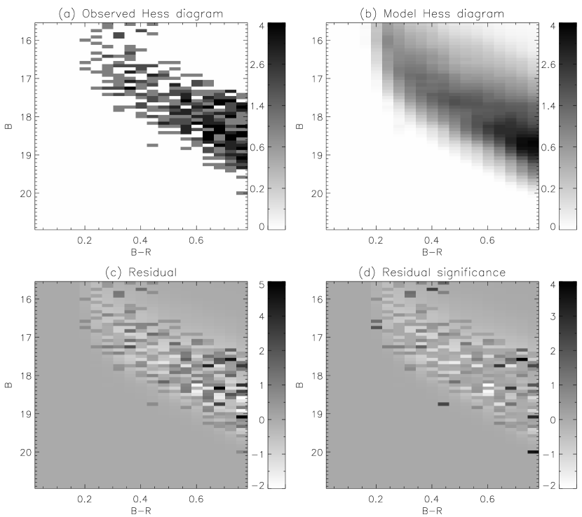
Figure 6.— Like Figure 5 but for the best SC fit to the YMS in field C2.

Our fit results for the OMS in the different fields are in very good agreement with each other. The favored foreground extinction values are close to, but slightly higher than the values from Schlegel, Finkbeiner & Davis (1998) for all fields. All fields favor a mean stellar age of $\sim$3-6 Gyr, but the exact age and age spread of the OMS population are not well constrained. For example, some SCs with an age range of 5 to 12 Gyr give acceptable fits. Given the large amount of contamination in these fields, the existence of less numerous populations of different ages (for example ‘ancient’ stars) cannot be excluded. Also, for none of the fields we can make a statistically significant distinction between models with small or very large age spread. An exact age and age spread would have to be derived from the exact location and width of the MSTO in magnitude. Because the MSTO region is heavily contaminated by halo and thick disk stars and because of the l.o.s. extent of CMa this information is largely lost.

The metallicity is constrained better by these fits and gives [Fe/H]$\sim$-1.0 for the central fields and [Fe/H]$\sim$-0.6 for the outer fields. This might hint at a metallicity gradient within CMa, but owing to the rather large uncertainties on the metallicities of the outer fields, significance of this is low. The best-fit values for the central fields agree very well with the spectroscopic metallicity measurements from N.F. Martin et al. (2007, in preparation). They obtained FLAMES and AAOMEGA spectra of several hundred Red Clump stars in several pointings within a few degrees of the center of CMa. For the kinematically selected CMa members they find [Fe/H]=-0.9 with a spread of $\sim$0.2 dex. Our estimates for the outer fields agree well with the metallicity found by Carraro et al. (2006) for the old stellar population in a field at ($l$,$b$)=(232°,-6°).

The distance moduli found for fields C1, C2, O1, and O2 correspond to distances of 7.4, 7.9, 6.9, and 7.2 kpc respectively, in good agreement with previous estimates, which range from 6.9 to 8.0 kpc (Bellazzini et al., 2004; Martin et al., 2004b; Martinez-Delgado et al., 2005; Bellazzini et al., 2006).

The l.o.s. depth of the CMa over-density (reflected in the OMS dispersion in magnitudes) shows the same picture in all fields, with an average best-fit value of 0.42 magnitudes. The observed MS width is not only caused by the spread along the l.o.s. but is also due to the intrinsic metallicity spread of the stars, differential reddening, and binary stars. The best-fit extinctions agree with the Schlegel, Finkbeiner & Davis (1998) values implying that practically all extincting material seems to be located between us and the over-density, not within the over-density. With a realistic binary fraction and a metallicity spread of 0.2 in [Fe/H], similar to the spread measured spectroscopically by N.F. Martin et al. (2007, in preparation), our model CMDs indicate that the majority of the observed OMS width reflects the l.o.s. extent of the CMa over-density. Of course, the corresponding physical half-width, $\sigma_{los}$, in kpc depends on the absolute distance, and is 1.5 kpc at 7.5 kpc.

Also the SC fit results for the YMS are internally consistent. Again the extinction values are close to the Schlegel, Finkbeiner & Davis (1998) values, although now slightly lower. Since the YMS is expected to be equidistant with or behind the OMS rather than in front of it, the extinction towards the YMS can of course not be lower than towards the OMS in reality.

Despite the fact that for the YMS no distinct MSTO is observed, the ages are better constrained than for the OMS, because contamination by fore- and background stars is not a serious problem. All fits within 1$\sigma$ of the best fit have an upper age limit Age_ul of 2 Gyr. Moreover, in the case of field C2, all acceptable fits have the same age bin of 0.25-2 Gyr, meaning that all other age bins give fits that are at least 1$\sigma$ worse than the best fit. For both fields the oldest age bin (2 to 5 Gyr) is excluded with more than 99% confidence, arguing a posteriori that a distinction of OMS and YMS is sensible. Also all age bins with an Age_ul less than 100 Myr are excluded with more than 99% confidence. According to our results, the youngest stars in the YMS must be at least as young as $\sim$700 Myr and the oldest at most 2 Gyr old. Thus, from our fits the YMS seems to consist of stars with ages between a few hundred million years and 2 Gyr. These estimates agree with those of Bellazzini et al. (2004), but are older than found by Carraro et al. (2005) and Moitinho et al. (2006).

The best-fit metallicity is more metal-rich than that of the OMS, [Fe/H]$\sim$-0.3, and in that case the YMS is somewhat more distant than the OMS, namely 9.1 and 9.5 kpc in C1 and C2, respectively, but with large uncertainties. As will be discussed in more detail below, due to the degeneracy between these parameters, they are not well constrained individually. The measured l.o.s. dispersion in field C1 is similar to that of the OMS, but a bit smaller in field C2. At their respective best-fitting distances the recovered l.o.s. dispersions for the YMS in C1 and C2 correspond to a $\sigma_{los}$ of $\sim$1.8 kpc and $\sim$1.3 kpc.

Based on the best-fit parameters from Table 2 we can reconstruct what the CMDs of our fields would look like if there were only CMa stars present without any contamination by fore- and background stars. Using the isochrones from Girardi et al. (2002), assuming a standard Salpeter IMF, and applying the photometric errors and completeness of our data, gives realistic representations of our best-fit SC models. The resulting CMDs in Figure 8 show an approximate, ‘clean’ picture of the CMa overdensity in fields C1, C2, O1 and O2. Comparing Figure 8 with Figure 3 nicely illustrates the amount of contamination we have to deal with.

3.3. Distance-metallicity degeneracy

One of the key questions in the CMa debate is whether the young and old stellar over-densities are physically related or not. Although the values in Table 2 suggest at first glance that the YMS may actually be farther away and half a dex more metal-rich than the OMS, the degeneracy between metallicity and distance prohibits a secure determination of this. Figure 7 shows the goodness-of-fit contours in the metallicity vs. distance modulus plane for the YMS (dashed) and OMS (solid) in fields C1 and C2. To remove another degeneracy, the foreground extinction was fixed to 1.1 for C1 and 0.7 for C2, but all age bins and $\sigma_{los}$ bins were included for making these plots. The direction of the degeneracy is obvious, with the best-fit distance increasing for increasing metallicity. While for these foreground extinction values the metallicity of the OMS is relatively robustly determined at [Fe/H]=-0.8, the metallicity constraint for the YMS is not strong. If the YMS is significantly more metal-rich than the OMS, it must be more distant. However, as the contours in Figure 7 indicate, our fits are also consistent with the YMS having a similar metallicity to the OMS, in which case it would be at the same distance as the OMS.

Figure 7.— Contour plots of the goodness-of-fit as function of metallicity and distance modulus of the SC fits in fields C1 (left) and C2 (right). The 1 and 3 $\sigma$ contours are plotted with solid lines for the OMS and with dashed lines for the YMS. Only SC fits with foreground extinction of $A_{V}$=1.1 and $A_{V}$=0.7 for C1 and C2 respectively were used to construct the contours.

Figure 8.— Model CMDs of the Canis Major over-density for the fields analyzed in this study. The reconstructions are based on the best-fit values for the OMS and YMS in Table 2 and the isochrones from Girardi et al. (2002) and include the photometric errors and completeness determined from the artificial star tests. Also the number of stars in the CMDs is scaled to reproduce realistic models of what the CMDs in Figure 3 would look like in the absence of fore- and background stars.

4. Combined distance solutions

While in the previous sections the YMS and OMS populations were treated separately, we now proceed to fit the complete CMDs of fields C1 and C2. Using the distance fitting mode of MATCH (see section 2.2) we will try to confirm the distances obtained in the previous section and look again at the possible distance offset between the two populations.

In the distance fitting mode of the MATCH fitting, the age bins to be used have to be specified as well as a fixed metallicity for each age bin. We use eight age bins with limits in log(years) of 7.5 to 8.0, 8.0 to 8.5, 8.5 to 9.0, 9.0 to 9.3, 9.3 to 9.5, 9.5 to 9.7, 9.7 to 9.9 and 9.9 to 10.1. Based on the results from the previous section we expect to find YMS stars in some of the four youngest age bins and OMS stars in some of the four oldest. As the YMS metallicity is not well constrained, we consider two cases. In the first case we assign metallicities of [Fe/H]=-1.0 to the four oldest bins, the best-fit value from our SC fits to the OMS that is consistent with the spectroscopic metallicities, and metallicities of [Fe/H]=-0.3 to the four youngest bins. In the second case we assign the same metallicity, [Fe/H]=-0.85, to all age bins. The extinction is fixed at an $A_{V}$ of 1.0 for C1 and 0.7 for C2 and we apply a Gaussian distance modulus spread of 0.5 magnitudes. We use the same control field CMDs as for the SC fits to the OMS in fields C1 and C2.

Figure 9 shows the results of the distance fits for field C1, for the case of metal-poor OMS and metal-rich YMS (left column), and for a uniform metallicity over the whole age range (right column). The upper panels show the distance solutions as 2-D histograms and the middle and lower panels show the corresponding synthetic Hess diagrams and residual significances. In Figure 10 we show the same results for field C2. The results are in agreement with those of the previous section. Assuming a metallicity of [Fe/H]=-1.0 for the oldest age bins and [Fe/H]=-0.3 for the youngest, the OMS stars are located at the same distance moduli that the SC fits give, and the YMS stars are located at distance moduli that are $\sim$0.6 magnitudes larger. Because of the l.o.s. extent of both populations, they do partly overlap in space, but their density peaks are clearly not equidistant in the case of differing metallicities. As already implied by Figure 7, when assuming a constant metallicity of [Fe/H]=-0.85 over the whole age range, the YMS is found to be at the same distance as the YMS. Comparing the model Hess diagrams and residual significance plots in Figures 9 and 10 shows that both scenarios give practically indistinguishable fits.

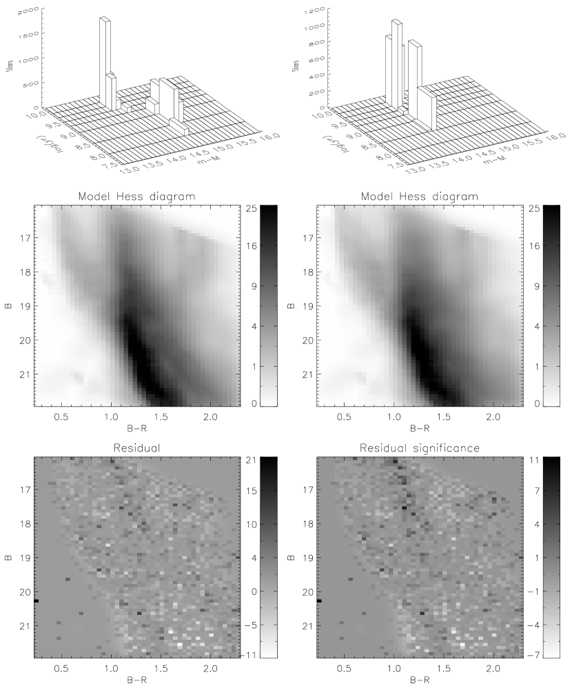
Figure 9.— Distance fitting results for the complete CMD of field C1. Left: for the plots in this column, a metallicity of [Fe/H]=-1.0 was assumed for the four oldest age bins and [Fe/H]=-0.3 for the four youngest age bins. Right: for this column a metallicity of [Fe/H]=-0.85 was assumed for all age bins. Top: best distance-age solution as 2-D histogram showing the number of stars in each distance-age bin needed to best reproduce the observed CMD; the background CMD is scaled to account for the fore- and background stars, meaning that the stars in these bins represent only the stars in the stellar over-density. Middle: the synthetic CMDs corresponding to the distance-age solution plotted in the top panels plus the background. Bottom: significance of the residuals between the observed and synthetic Hess diagrams. Overall this shows a random scatter with only very small systematic deviations. In the bottom-left part (B$>$20, B-R$<$1) there are some pixels with high significance where stars are located in the control field but not in the target field. Such pixels do not influence the fitting since none of the probed model populations can reproduce these stars.

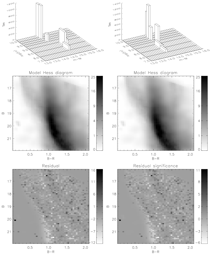
Figure 10.— As Figure 9, but for field C2.

5. Discussion

Before discussing the implications of our results for the interpretation of the CMa stellar over-density, it is worthwhile to review these results.

5.1. Overview of results

We have investigated the stellar populations of the CMa over-density in several fields using deep optical photometry and CMD fitting techniques. Specifically, we explored the properties of the OMS and YMS using SC fits in Section 3. For the fields near the presumed center of CMa the fits indicate a rather low metallicity of [Fe/H]$\sim$-1.0$\pm$0.1 dex for the OMS. This agrees well with the spectroscopic measurements from N.F. Martin et al. (2007, in preparation), [Fe/H]$\simeq$-0.9, based on several hundred RC stars within a few degrees from the positions of our central fields. The distance we measure to the OMS is 7.4, 7.9, 6.9, and 7.2 kpc for fields C1, C2, O1, and O2 respectively, which also agrees well with previous estimates (Bellazzini et al., 2004; Martin et al., 2004b; Martinez-Delgado et al., 2005; Bellazzini et al., 2006). We find a $\sigma_{los}$ of $\sim$0.42 magnitudes. Since the photometric errors, age and metallicity spread, and a realistic binary fraction are all accounted for in the models, this directly translates into a physical l.o.s. depth of $\sim$1.5 kpc. This is consistent with our upper limit for $\sigma_{los}$ for the OMS in B06. The exact stellar ages and age distribution within the OMS population cannot be constrained well because of the heavy contamination by fore- and background stars in the MSTO region. But we find that the OMS population is predominantly $\sim$3-6 Gyr old, which is typically termed an ‘intermediate’ age. Given the amount of contamination in the fields this, however, does not exclude the presence of a less numerous population of, for example, much older stars.

For the YMS the ages are better constrained and these stars have a range in age from at least few hundred million years to at most $\sim$2 Gyr. Based on our results we conclude with high significance that the YMS stars cannot all be younger than 100 Myr, nor older than 2 Gyr. Owing to a strong degeneracy between metallicity and distance modulus (see Figure 7), a secure determination of either of these parameters individually is precluded. Either the YMS has a metallicity similar to that of the OMS, in which case it would have to be equidistant and therefore co-spatial with the OMS, or it is more metal-rich, in which case it is located behind the OMS. This same picture is confirmed by our distance solution fits in Section 4.

5.2. Implications for the nature of CMa

How do our findings relate to the hypotheses that have been put forward to explain the CMa over-density? Since the possibility exists that the OMS and YMS populations are not actually related, it should be considered that different explanations are needed for each. Three theories have been suggested in the literature: (a) the CMa over-density is (the remnant of) an dwarf galaxy being accreted onto the MW (e.g. Martin et al., 2004b; Bellazzini et al., 2004; Martin et al., 2005; Bellazzini et al., 2005; Martinez-Delgado et al., 2005; Bellazzini et al., 2006); (b) the warp and flare of the outer disk create the observed over-density along the l.o.s. (Momany et al., 2004, 2006); (c) both OMS and YMS are related to intrinsic substructure within the outer disk, the OMS to a nearby spiral arm and the YMS to a distant spiral arm (Carraro et al., 2005; Moitinho et al., 2006). Below we discuss each of these options in light of the results of this paper.

If the CMa over-density is an accreted dwarf galaxy, it would be expected to have different properties from disk stars, for example in kinematics and metallicity. Proper motion measurements of a sample of YMS stars near the presumed center of CMa by Dinescu et al. (2005) are consistent with this scenario (Peñarrubia et al., 2005), as are kinematical measurements of the OMS by Martin et al. (2004b) and Martin et al. (2005). Recent metallicity measurements of stars in the outer galactic disk by Yong et al. (2006) show a clear dependence on galactocentric radius ($R_{GC}$). Our determination of the metallicity of the OMS stars of [Fe/H]$\sim$-1.0 means that they are significantly more metal-poor than the expectation for disk stars at $R_{GC}\sim$13 kpc, [Fe/H]$\approx$-0.5 (Yong et al., 2006), thus hinting at an external origin. The ages of the OMS stars are not well constrained, but the majority of the population has an intermediate age of $\sim$3-6 Gyr. Many dwarf galaxies have such intermediate age populations, but are expected to also contain a population of older ($\sim$10 Gyr) stars; but as mentioned before our results do not exclude the presence of such stars. The SC fits are sensitive to the most numerous population and a less numerous population could easily ‘hide’ in the noise caused by the large contamination from fore- and background stars. Unfortunately, photometry alone does not constrain the metallicity of the YMS stars well enough and therefore we cannot say whether or not their metallicity is consistent with them being disk stars. Should they have similar metallicities to the OMS stars, it would be hard to reconcile this with them being disk stars. Furthermore, it would place them at the same distance as the OMS stars (e.g. Figure 7), in accordance with the picture of an accreted dwarf galaxy with an extended star formation history. On the other hand, they might be metal-rich and farther away than the OMS, meaning that the two populations are probably not related at all. In this case, the metallicity and kinematics of the OMS would still be consistent with an external origin, but the YMS might well originate in the Galaxy. Spectroscopic measurements of YMS stars will clearly be of key importance to resolve this issue.

In B06 we compare the observed stellar density profile along the l.o.s. towards Canis Major with predictions from Galactic warp/flare models. This analysis shows that the warp of the outer disk is unlikely to produce as narrow a peak in the stellar density at a distance of $\sim$7.5 kpc as is observed. Rather, a more extended density peak is expected, peaking much closer to us. The distance and $\sigma_{los}$ determinations in this paper confirm that the l.o.s. density profile of CMa has a narrow peak with $\sigma_{los}\simeq$1.5 kpc centered at $\sim$7.5 kpc and are thus inconsistent with the warp interpretation of CMa. As stated before, the metallicity we find for the OMS is significantly lower than expected for disk stars, also arguing against the warp/flare hypothesis. Although the YMS stars might be disk stars, their distance ($\sim$9.3 kpc in this case) is also inconsistent with smooth (locally axisymmetric) warp models. Additional substructure would have to be invoked to explain an over-density of young stars at this distance.

Large scale substructure in the disk exists in the form of spiral arms, and especially young stellar populations are concentrated in these. Moitinho et al. (2006) suggest that the young stars seen in the direction of Canis Major and in the background of several open clusters are part of the outer Norma-Cygnus spiral arm. In their picture, the old stars are part of the Orion (Local) arm, which is located in the inter-arm region between the Sagittarius and Perseus spiral arms, meaning that the old stars are much closer to us. If the YMS is part of a Galactic spiral arm it should be expected to be relatively metal-rich. Assuming [Fe/H]=-0.3, our fits imply a distance to the YMS of $\sim$9 kpc. Figure 11 shows a schematic face-on view of the third quadrant of the Milky Way. Spiral arms according to Vallee (2005), which are based on a combination of different optical and HI spiral arm tracers, are outlined as well as the position of the sun and the l.o.s. towards the CMa fields studied in this paper. The black dot indicates the location of the YMS if [Fe/H]=-0.3; it coincides with the distance to the outer spiral arm. Our fits therefore confirm that when assuming close-to-solar metallicities one will find that the distance to the YMS is the same as the distance to the Norma-Cygnus spiral arm. It should be noted that although the YMS coincides with the spiral arm in this face-on view, it has a large offset in Z, the direction perpendicular to the plane. If this distance is correct, these YMS stars are located more than 1 kpc out of the plane of the disk. All “classic” tracers of the spiral arm are less than 0.5 kpc out of the Galactic midplane ($b$=0), with the exception of only one detected molecular cloud. The proper motion measurements by Dinescu et al. (2005) show that the YMS stars are moving even farther away from the plane. Some additional explanation for the extreme location and kinematics of these stars is needed to reconcile them with a Galactic origin. If we assume that the metallicity of the YMS is much lower than solar and similar to that of the OMS, the best-fit distance of the YMS shifts to the same distance as the OMS, in which case it is located in an inter-arm region. Again, spectroscopic measurement of the metallicity of the YMS is crucial to solve this problem.

The location of the OMS is indicated in Figure 11 with the dark grey dot; it lies in the inter-arm region between the Perseus and Cygnus spiral arms. Also drawn in Figure 11 is the approximate position of the Orion arm, as outlined by Moitinho et al. (2006) in their Figure 2, based on the positions of open star clusters. Clearly, the Orion arm crosses the l.o.s. towards our fields at a much smaller distance of approximately 2 kpc, or a distance modulus of m-M=11.5. Such a distance is far smaller than what previous studies of CMa have indicated and excluded at high confidence by our results (see e.g. Table 2 and Figure 7). Furthermore, the metallicity we find for the OMS in fields C1 and C2, [Fe/H]$\sim$-1.0, is much lower than is found for the Galactic thin and thick disk (e.g. Yong et al., 2006; Bensby et al., 2004).

Figure 11.— Schematic overview of the third quadrant of the MW, seen face-on from the North Galactic pole; the light-grey bands trace the spiral arms according to Vallee (2005), based on a combination of different spiral arm tracers. The position of the sun is indicated and the galactic center is at (0,0) in these $X,Y$ coordinates. Drawn as a solid line is the projection onto the Galactic plane of the l.o.s. towards the fields used in this paper ($l$=240°), and the approximate location of the local Orion arm is indicated with a dotted line. The grey and black circle and band indicate the peak distance and l.o.s. extent (assuming a symmetrical distribution along the l.o.s.) of the OMS and YMS, respectively, in the case that the YMS has [Fe/H]=-0.3 dex. Also plotted are the peak distances projected onto the Galactic plane, showing that for this metallicity the YMS is equidistant with the outer spiral arm.

6. Summary and Conclusions

Applying CMD-fitting techniques to a small subset of fields from our survey of the CMa region (B06) we have determined the distance, l.o.s. extent and metallicity of the old and young stars in the CMa over-density. For the “old” stars (OMS) the recovered distance, $\sim$7.5 kpc, $\sigma_{los}$, $\sim$1.5 kpc, metallicity, [Fe/H]$\sim$-1.0, and mean ages, $\sim$3-6 Gyr, are in good agreement with results from the literature. Also, we have constrained the metallicity, distance, l.o.s. extent and ages of the younger population of stars seen in the same direction. These stars have ages of at least a few hundred million years and at most 2 Gyr. The degeneracy between distance and metallicity prevents us from drawing a firm conclusion about the co-spatiality of the old and young stars. A metal-rich ([Fe/H]=$\sim$-0.3) population at $\sim$9.3 kpc and a metal-poor ([Fe/H]=$\sim$-0.8) population at 7.5 kpc are both consistent with the data. Spectroscopic metallicities for the young stars are necessary to distinguish between these two possibilities.

A comparison of the distance of the OMS with Galactic warp/flare models argues against the interpretation that the OMS is the result of the warp and flare of the Galactic disk (B06). Our results are inconsistent with the OMS stars being located in the local Orion arm, since the implied distance of $\sim$2 kpc is ruled out with high significance. The metallicity we find seems too low for disk stars, hinting at an external origin. Because of the degeneracy mentioned above we cannot be certain about the nature of the YMS. If it is metal-rich, it coincides in distance, but not in height above the disk, with the Norma-Cygnus spiral arm. Perhaps a scenario where a combination of spiral arm structure and the warp conspire to produce young stars so far out of the disk is feasible. On the other hand, if the YMS has a similar metallicity to the OMS, it is co-spatial with the OMS and located in an inter-arm region. In this case, the accreted dwarf galaxy scenario would be the more likely explanation.

References

- Aparicio, Gallart & Bertelli (1997) Aparicio, A., Gallart, C. & Bertelli, G. 1997, AJ, 114, 680
- Bellazzini et al. (2004) Bellazzini, M., Ibata, R., Monaco, L., Martin, N., Irwin, M. J., Lewis, G. F., 2004, MNRAS, 354, 1263
- Bellazzini et al. (2005) Bellazzini, M., Ibata, R. A., Monaco, L., Martin, N., Irwin, M. J., et al. 2005, MNRAS, 354, 1263
- Bellazzini et al. (2006) Bellazzini, M., Ibata, R. A., Martin, N., Lewis, G. F., Conn, B., Irwin, M. J., 2006, MNRAS, 366, 865
- Bensby et al. (2004) Bensby, T., Feltzing, S. & Lundström, I., 2004, A&A, 421, 969
- Bertin & Arnouts (1996) Bertin, E. & Arnouts, S., 1996, A&AS, 117, 393
- Bonifacio et al. (2000) Bonifacio, P., Monai, S., Beers, T. C., 2000, AJ, 120, 2065
- Butler et al. (2006) Butler, D. J., Martinez-Delgado, D., Rix, H-W., Peñarrubia, J., De Jong, J. T. A., 2006, subm., astro-ph/0609316, B06
- Carraro et al. (2005) Carraro, G., Vázquez, R. A., Moitinho, A. & Baume, G., 2005, ApJ, 630, L153
- Carraro et al. (2006) Carraro, G., Moitinho, A., Zoccali, M., Vázquez, R. A. & Baume, G., 2006, AJ, in press, astro-ph/0610617
- Dinescu et al. (2005) Dinescu, D. I., Martínez-Delgado, D., Girardi, T. M., Peñarrubia, J., Rix, H.-W., Butler, D. J., van Altena, W. F., 2006, ApJ, 631, L49
- Dolphin (1997) Dolphin, A. E. 1997, New A, 2, 397
- Dolphin (2002) Dolphin, A. E. 2002, MNRAS, 332, 91
- Duquennoy & Mayor (1991) Duquennoy, A. & Mayor, M., 1991, A&A, 248, 485
- Gallart et al. (1996) Gallart, C., Aparicio, A., Bertelli, G., Chiosi, C. 1996, AJ, 112, 1950
- Girardi et al. (2002) Girardi, L., Bertelli, G., Bressan, A., Chiosi, C., Groenewegen, M. A. T., Marigo, P., Salasnich, B. & Weiss, A., 2002, A&A, 391, 195
- Harris & Zaritsky (2001) Harris, J. & Zaritsky, D. 2001, ApJS, 136, 25
- Hernandez, Gilmore & Valls-Gabaud (2000) Hernandez, X., Gilmore, G. & Valls-Gabaud, D. 2000, MNRAS, 317, 831
- Holtzman et al. (1999) Holtzman, J. A. et al., 1999, AJ, 118, 2262
- Kroupa et al. (1993) Kroupa, P., Tout, C. A. & Gilmore, G., 1993, MNRAS, 262, 545
- Martin et al. (2004a) Martin, N. F., Ibata, R. A., Bellazzini, M., Irwin, M. J., Lewis, G. F., Dehnen, W., 2004a, MNRAS, 348, 12
- Martin et al. (2004b) Martin, N. F., Ibata, R. A., Conn, B. C., Lewis, G. F., Bellazzini, M., Irwin, M. J., McConnachie, A. W., 2004b, MNRAS, 355, L33
- Martin et al. (2005) Martin, N. F., Ibata, R. A., Conn, B. C., Lewis, G. F., Bellazzini, M., Irwin, M. J., 2005, MNRAS, 362, 906
- Martinez-Delgado et al. (2005) Martínez-Delgado, D., Butler, D. J., Rix, H-W., Franco, Y. I., Peñarrubia, J., 2005, ApJ, 633, 205
- Moitinho et al. (2006) Moitinho, A., Vázquez, R. A., Carraro, G., Baume, G., Giorgi, E. E., Lyra, W., 2006, MNRAS, 368, L77
- Momany et al. (2004) Momany, Y., Zaggia, R. S., Bonifacio, P., Piotto, G., De Angeli, F., Bedin, L. R., Carraro, G., 2004, A&A, 421, L29
- Momany et al. (2006) Momany, Y., Zaggia, R. S., Gilmore, G., Piotto, G., Carraro, G., Bedin, L. R., De Angeli, F., 2006, A&A, 451, 515
- Newberg et al. (2002) Newberg, H. J., Yanny, B., Rockosi, C., Grebel, E. K., Rix, H-W., et al., 2002, ApJ, 569, 245
- Olsen (1999) Olsen, K. A. G. 1999, AJ, 117, 2244
- Peñarrubia et al. (2005) Peñarrubia, J., Martínez-Delgado, D., Rix, H. W., Gómez-Flechoso, M. A., Munn, J., 2005, ApJ, 626, 128
- Rocha-Pinto et al. (2006) Rocha-Pinto, H. J., Majewski, S. R., Skrutskie, M. F., Patterson, R. J., Nakanishi, H., Muñoz, R. R., Sofue, Y., 2006, ApJ, 640, L147
- Schirmer et al. (2003) Schirmer, M., Erben, T., Schneider, P., Pietrzynski, G., Gieren, W., 2003, A&A, 407, 869
- Schlegel, Finkbeiner & Davis (1998) Schlegel, D., Finkbeiner, D. & Davis, M. 1998, ApJ, 500, 525
- Tolstoy & Saha (1996) Tolstoy, E. & Saha, A. 1996, ApJ, 462, 672
- Vallee (2005) Vallee, J. P., 2005, AJ, 130, 569
- Yanny et al. (2003) Yanny, B., Newberg, H. J., Grebel, E. K., Kent, S., Odenkirchen, M., 2003, ApJ, 588, 824
- Yong et al. (2006) Yong, D., Carney, B. W., Teixera de Almeida, M. L., Pohl, B. L., 2006, AJ, 131, 2256