Simulations of star formation in a gaseous disc around Sgr A^∗– a failed Active Galactic Nucleus

Abstract

We numerically model fragmentation of a gravitationally unstable gaseous disc under conditions that may be appropriate for the formation of the young massive stars observed in the central parsec of our Galaxy. In this study, we adopt a simple prescription with a locally constant cooling time. We find that, for cooling times just short enough to induce disc fragmentation, stars form with a top-heavy Initial Mass Function (IMF), as observed in the Galactic Centre (GC). For shorter cooling times, the disc fragments much more vigorously, leading to lower average stellar masses. Thermal feedback associated with gas accretion onto protostars slows down disc fragmentation, as predicted by some analytical models. We also simulate the fragmentation of a gas stream on an eccentric orbit in a combined Sgr A^∗ plus stellar cusp gravitational potential. The stream precesses, self-collides and forms stars with a top-heavy IMF. None of our models produces large enough co-moving groups of stars that could account for the observed “mini star cluster” IRS13E in the GC. In all of the gravitationally unstable disc models that we explored, star formation takes place too fast to allow any gas accretion onto the central super-massive black hole. While this can help to explain the quiescence of ‘failed AGN’ such as Sgr A^∗, it poses a challenge for understanding the high gas accretion rates infered for many quasars.

1 Introduction

There is no detailed understanding of how super-massive black holes (SMBHs) gain their mass, except that it must be mainly through gaseous disc accretion (Yu & Tremaine, 2002). The standard accretion disc model (Shakura & Sunyaev, 1973) shows that accretion discs must be quite massive and cold at “large” (sub-parsec in this context) distances from the SMBH. Many theorists pointed out that these discs should be unstable to self-gravity, and thus must form stars or giant planets by gravitational fragmentation (e.g., Paczyński, 1978; Kolykhalov & Sunyaev, 1980; Shlosman & Begelman, 1989; Collin & Zahn, 1999; Bertin & Lodato, 1999; Gammie, 2001). This creates a dilemma for the field, as star formation might be a dynamical, very fast process which may result in a complete transformation of the gas into stars. The SMBH would then be starved of fuel. Goodman (2003); Sirko & Goodman (2003) have recently demonstrated that star formation cannot be quenched by stellar feedback, unless one is prepared to grossly violate constraints that we have from AGN spectra.

Goodman (2003) suggested that the feeding of SMBHs proceeds via direct accretion of low angular momentum gas that settles in a small scale disc. Such a disc would be too hot to allow star formation. The size of this “no-star-formation region” is $R\lower 2.15277pt\hbox{$\;\buildrel<\over{\sim}\;$}0.03$ pc, and is weakly dependent on the SMBH mass. However, one realistically expects that an even larger amount of gas settles at larger radii where it could collapse and form stars, or it could accrete on the SMBH. Therefore the fate of these self-gravitating discs is still very much interesting.

Current observations provide new impetus for theoretical work on the topic. Wehner & Harris (2006); Ferrarese et al. (2006) have shown that many galaxies host “extremely compact nuclei” (ECN) – star clusters located in the very central $\sim 5$ parsec of galaxies. Closer to home, in the centre of our Galaxy, about a hundred massive young stars, mostly arranged into two stellar discs of $\sim 0.05$–0.5 parsec scale (Levin & Beloborodov, 2003; Genzel et al., 2003; Paumard et al., 2006), circle the super-massive black hole named Sgr A^∗. These stars are suspected to have been formed in situ, as evidenced by the lack of stars outside the $\sim 0.5$ parsec region (Paumard et al., 2006; Nayakshin & Sunyaev, 2005). Several observational facts are consistent with the hypothesis that these stars formed in a massive gaseous disc (Paumard et al., 2006). Had this star formation event not happened, Sgr A^∗ could have been accreting gas from the gaseous disc even now. Sgr A^∗ thus failed to realise itself as an AGN because of the loss of gas to star formation (Nayakshin & Cuadra, 2005).

A number of important gaps in our understanding of young stars near Sgr A^∗ remain. The counter clock-wise disc appears to host stars on more elliptical orbits, and it is also geometrically thicker. The same disc also contains a puzzling “mini star cluster”, IRS13E, that consists of more than a dozen stars and may be bound by an Intermediate Mass Black Hole (IMBH) of mass ${\,{M}_{\rm bh}}\lower 2.15277pt\hbox{$\;\buildrel>\over{\sim}\;$}10^{3}{\,{\rm M}_{\odot}}$ (Paumard et al., 2005; Schödel et al., 2005). The IMF of the observed stars must be top-heavy according to several lines of evidence (Nayakshin & Sunyaev, 2005; Nayakshin et al., 2006; Paumard et al., 2006; Alexander et al., 2006), which is not expected in the most basic model of a fragmenting disc, as the Jeans mass there is significantly sub-solar (e.g., Levin 2006, Nayakshin 2006, but see also Larson 2006).

In this paper, we discuss numerical simulations of star formation occurring in a gaseous disc around Sgr A^∗. Given the numerical challenges in the problem, we foresee that a reliable modelling of all the questions raised by the young stars near Sgr A^∗ will require an extended effort of constantly increasing complexity. In this study we present numerical experiments with a locally constant cooling time. This allows a convenient comparison with previous analytical and numerical works that predicted the conditions when fragmentation should take place. It might also form a basis for comparison with future work.

Within our formalism with a locally constant cooling time, we find that (i) circular and eccentric discs alike can gravitationally fragment and form stars; (ii) the IMF of formed stars is a strong function of cooling time, becoming top-heavy for marginally star-forming discs; (iii) star formation feedback is indeed able to slow down disc fragmentation, as suggested by several earlier analytical papers, but it is not yet clear if it can alleviate the fueling problem of the SMBHs; (iv) our simulations do form some tightly bound binary stars but more populous systems (a la IRS13E) do not survive long.

This paper is structured as follows. In Section 2, we discuss our simulation methodology and the basic conditions for disc fragmentation. Section 3 explains our sink particle approach to treat star formation in more detail. We then analyse the evolution after disc fragmentation and the IMF of the formed stars in Section 4. The sensitivity of our results to numerical resolution and feedback from stars is discussed in Sections 5 and 6, respectively. We then examine elliptical orbits of a gaseous stream in Section 7, and the question of the formation of mini star-clusters in Section 8. Finally, we summarize and conclude in Section 9.

2 Methods and disc fragmentation tests

We use the SPH/$N$-body code GADGET-2 (Springel et al., 2001; Springel, 2005) to simulate the dynamics of stars and gas in the (Newtonian) gravitational field of a point mass with ${\,{M}_{\rm bh}}=3.5\times 10^{6}{\,{\rm M}_{\odot}}$. The code solves for the gas hydrodynamics via the smoothed particle hydrodynamics (SPH) formalism. The hydrodynamic treatment of the gas includes adiabatic processes and artificial bulk viscosity to resolve shocks. The stars are modelled as sink particles, using the approach developed by Springel et al. (2005), modified in the ways described below.

Table 1 lists some of the parameters and results of the simulations presented in this paper. The tests described in this section are those listed as S1–S5 (the “S” stands for “standard”). The units of length and mass used in the simulations are $R_{\rm U}=1.2\times 10^{17}\hbox{cm}\approx 0.04$ pc, which is equal to $1^{\prime\prime}$ at the 8.0 kpc distance to the GC, and $M_{\rm U}=3.5\times 10^{6}{\,{\rm M}_{\odot}}$, the mass of Sgr A* (e.g., Schödel et al., 2002), respectively. The dimensionless time unit is $t_{\rm U}=1/\Omega(R_{\rm U})$, or about 60 years ($\Omega$ is defined just below Eqn. 1). The masses of SPH particles are typically around $0.01$ Solar masses (see Table 1).

2.1 Gravitational collapse

Toomre (1964) showed that a rotating disc is subject to gravitational instabilities when the $Q$-parameter

$$Q=\frac{\Omega^{2}}{2\pi G\rho}$$ (1)

becomes smaller than a critical value, which is close to unity. This form of the equation assumes hydrostatic equilibrium to relate the disc sound speed to its vertical thickness, $H$. $\Omega=(G{\,{M}_{\rm bh}}/R^{3})^{1/2}$ is the Keplerian angular frequency, and $\rho$ is the vertically averaged disc density. Gravitational collapse thus takes place when the gas density exceeds

$$\rho_{\rm BH}\equiv\frac{\Omega^{2}}{2\pi G}\;.$$ (2)

Ideally, numerical simulations should resolve the gravitational collapse down to stellar scales. In practice, this is impossible for numerical reasons, and instead collisionless “sink particles” are commonly introduced (Bate et al., 1995) to model collapsing regions of very high density. To ensure that collapse is well under way when we introduce a sink particle, we require that the gas density exceeds

$$\rho_{\rm crit}=\rho_{0}+A_{\rm col}\rho_{\rm BH}\;,$$ (3)

where $\rho_{0}=5\times 10^{-11}$ g cm^-3, and $A_{\rm col}$ is a large number (we tested values from a few to a few thousand). We in general find that our results are not sensitive to the exact values of $\rho_{0}$ and $A_{\rm col}$, provided they are large enough (Section 5.2). Further details of our sink particle treatment are given in Section 3.1.

2.2 Gas cooling

We account for radiative cooling via a simple approach with a locally constant cooling time. The cooling term in the energy equation is

$$\left(\frac{{\rm d}u}{{\rm d}t}\right)_{\rm cool}\;=\;-\;\frac{u}{t_{\rm cool}(R)}\;,$$ (4)

where $u$ is the internal energy of an SPH particle, and $R$ is the radial location of the SPH particle, i.e. the distance to the SMBH. We parameterize the cooling time as a fixed fraction of the local dynamical time,

$$t_{\rm cool}(R)=\beta\times t_{\rm dyn}(R)\;,$$ (5)

where $t_{\rm dyn}=1/\Omega$ and $\beta$ is a parameter of the simulations. This simple model allows for a convenient validation of the simulation methodology as such locally constant cooling time models were investigated in detail in previous literature. Gammie (2001) has shown that self-gravitating discs are bound to collapse if the cooling time, $t_{\rm cool}$, is shorter than about $3/\Omega$ (i.e., $\beta<3$). Rice et al. (2005) presented a range of runs that tested this fragmentation criterion in detail, and found that, for the adiabatic index of $\gamma=5/3$ (as used throughout this paper), the disk fragments as long as $\beta\leq 6$.

Note that most of the simulations explored in this paper are performed for circular initial gas orbits, and also for relatively small disc (total gas) masses as compared with that of the SMBH. As will become clear later, this implies that during the simulations gas particles continue to follow nearly circular orbits, and thus their cooling time is constant around their orbits. One exception to this is a test done with eccentric initial gas orbits (Section 7).

2.3 Fragmentation tests

To compare our numerical approach with known results, we ran several tests (S1–S5 in Table 1) in a setup reminiscent of that of Rice et al. (2005), who modelled fragmentation of proto-stellar discs. One key difference between marginally self-gravitating proto-stellar and AGN discs is the relative disc mass. Whereas the former become self-gravitating for a disc to central object mass ratio of $M_{\rm disc}/M_{*}\sim 0.1-0.5$ (e.g., Rafikov, 2005), where $M_{*}$ is the mass of the central star, the latter become self-gravitating for a mass ratio as small as $M_{\rm disc}/{\,{M}_{\rm bh}}\simeq 0.003-0.01$ (e.g., Gammie, 2001; Goodman, 2003; Nayakshin & Cuadra, 2005; Levin, 2006). For marginally self-gravitating discs, the ratio of disc height to radius, $H/R$, is of order of the mass ratio, $H/R\sim M_{\rm disc}/{\,{M}_{\rm bh}}$ (Gammie, 2001). The disc viscous time is

$$t_{\rm visc}\sim\alpha^{-1}\left(\frac{R}{H}\right)^{2}\Omega^{-1}\;,$$ (6)

where $\alpha\sim 0.1-1$ is the effective viscosity parameter (Lin & Pringle, 1987; Gammie, 2001) for self-gravitating discs. Thus, for $H/R\lower 2.15277pt\hbox{$\;\buildrel<\over{\sim}\;$}0.01$, the disc viscous time is some 4–6 orders of magnitude longer than the disc dynamical time. This is in fact one of the reasons why the discs become self-gravitating, as they are not able to heat up quickly enough via viscous energy dissipation (Shlosman & Begelman, 1989; Gammie, 2001).

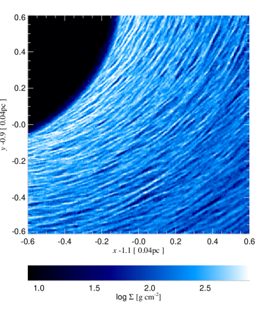
Figure 1: Surface density of a region in a marginally stable disc from the simulation S4 ($\beta=4.5$) at time $t=50$. The map is centred on the $(x,y)=(1.1,-0.9)$ location. Many small and somewhat dense gas clumps can be seen in the figure. None of the clumps however truly collapses, and most disappear on a dynamical time scale.

Also, since the disc viscous time is many orders of magnitude longer than the orbital time, as well as the total simulation time, we expect no radial re-distribution of gas in the simulations, and indeed very little occurs. Our models are essentially local, as emphasized by Nayakshin (2006), and hence it suffices to simulate a small radial region of the disc. For definiteness, we simulate a gaseous disc of mass $M_{\rm d}=3\times 10^{4}{\,{\rm M}_{\odot}}\approx 0.01{\,{M}_{\rm bh}}$ extending from $r_{\rm in}=1$ to $r_{\rm out}=4$, where $r$ is the dimensionless distance from Sgr A^∗.

The total initial number of SPH particles used in runs S1–S5 is $4\times 10^{6}$. Gravitational softening is adaptive, with a minimum gravitational softening length of $3\times 10^{-4}$ for gas, and $0.001$ for sink particles. The disk is in circular rotation around a SMBH with mass of ${\,{M}_{\rm bh}}=3.5\times 10^{6}{\,{\rm M}_{\odot}}$. The disc is extended vertically to a height of $H/R=0.02$ in the initial conditions, which renders it stable to self-gravity. As the gas settles into hydrostatic equilibrium, it heats up due to compressional heating, and then cools according to equation (4). We used five different values of $\beta=t_{\rm cool}\Omega$, in the runs, namely $\beta=0.3$, $2$, $3$, $4.5$ and $6$ (see Table 1).

The discs in runs with $\beta=0.3,2$ and 3 fragmented and formed stars, as expected based on the results of Rice et al. (2005), but our tests with $\beta=4.5$ and $6$ did not. However, the run with $\beta=4.5$ and $6$ did fragment in the sense of forming transient high density gas clumps, some of which can be noted in Figure 1. The maximum density in these clumps fluctuated between a few to a few dozen times $\rho_{\rm BH}$, i.e. the clumps were dense enough to be self-bound, but not dense enough for our sink particle criterion, since $A_{\rm col}$ was set to 30 for these tests (cf. Section 2.1).

Rice et al. (2005) reported fragmentation for values of $\beta$ as large as 6. This difference in the results is most likely due to our discs being much thinner geometrically. The high density structures formed in our simulations, like filaments and clumps, are much smaller in relative terms than they are in the simulations of proto-stellar discs. This is not surprising as the most unstable wavelength for the $Q\sim 1$ disc is of order of the disc vertical scale height $H$ (Toomre, 1964), and our discs are much thinner. Also, the high density structures are much more numerous in AGN discs. As analytically shown by Levin (2006), self-gravitating clumps in such discs are quite likely to collide with each other on a dynamical time scale. If clumps are tightly bound they may agglomerate. For tests with larger values of $\beta$, the clumps are marginally bound (as their maximum density exceeds $\rho_{\rm BH}$ by a factor of a few only), and any interaction may unbind them. In contrast, for high values of $H/R\sim M_{\rm disc}/M$, as appropriate for proto-stellar discs, fewer clumps form, and the interactions are probably too rare to cause clump destruction.

3 Star formation

3.1 Two types of sink particles

To design a physically reasonable and numerically sound procedure to deal with the gravitational collapse of cooling gas, we make use of well known results from the field of star formation. Simulations of collapsing gas haloes show that the first quasi-hydrostatic object to form has a characteristic size of about 5 AU, and may therefore be called a “first core” (e.g., Larson, 1969; Masunaga et al., 1998). As this optically thick gas condensation slowly cools, the core decreases in size while accreting mass from the infalling envelope. When the mass of the gas accumulated is of the order of $0.05$–$0.1{\,{\rm M}_{\odot}}$, H2 dissociation and hydrogen ionisation losses become efficient coolants, and the core can collapse dynamically to much higher densities and much smaller sizes (Larson, 1969; Silk, 1977). The relevant time scale is of the order of $\lower 2.15277pt\hbox{$\;\buildrel>\over{\sim}\;$}10^{3}$ years, which is very short compared with free fall times of typical molecular clouds in a galaxy. Creation of the first collapsed objects is therefore nearly instantaneous in a “normal” star forming environment, and their sizes are sufficiently small so that they can be considered point masses compared with the cloud size of $\sim 10^{18}$ cm.

The gas densities in self-gravitating AGN discs are $\rho/m_{\rm p}\sim 10^{8}-10^{12}$ cm^-3, i.e. many orders of magnitude larger than in galactic star forming regions, but smaller than the gas density of a first core, $\sim$ few $\times 10^{13}$ cm^-3. We assume that the initial stages of collapse should be similar to “normal” star formation except that it starts from higher initial gas densities. For Sgr A^∗, at the distance where the young massive stars are located (Paumard et al., 2006), the free-fall time in the collapsing gas clouds, $t_{\rm ff}\sim 1/(G\rho)^{1/2}\lower 2.15277pt\hbox{$\;\buildrel<\over{\sim}\;$}t_{\rm dyn}$, is of the order of 100–1000 years. For a more massive AGN, the time scales would be even shorter at comparable distances to the SMBH. The life-times of the first cores in this environment are then longer than the free-fall time, since the core collapse is dominated by the cooling time scale, which is much longer than the $t_{\rm ff}$ estimated above. This implies that these objects should actually be treated as having a finite life-time in our simulations. Furthermore, their sizes are only an order of magnitude smaller than that of the disc scale height, $H\sim 10^{15}$ cm (Nayakshin & Cuadra, 2005). Therefore, the first cores have a decent chance to merge with one another (Levin, 2006). They could also be disrupted by a more massive proto-star that passes by, form a disc and be subsequently accreted by the proto-star.

In order to capture this complicated situation in a numerically practical way, we introduce two kinds of sink particles. We call those with mass $M\leq M_{\rm core}=0.1{\,{\rm M}_{\odot}}$ “first cores”. Once the gas reaches the critical density (eq. 3), we turn SPH particles into sink particles individually, so the initial mass of a first core particle is equal to one SPH particle mass. First cores have geometrical sizes of $R_{\rm core}$, and can merge with one another if they pass within a distance smaller than $2f_{m}R_{\rm core}$ of each other, where $f_{m}\geq 1$ is a parameter that mimics the effect of gravitational focusing in mergers. We assume for simplicity that the lifetime of the first cores is longer than the duration of the simulations. We performed a few tests with finite core life times and found very similar results; most of the merging of first cores happens very quickly after they are created inside of a collapsing gas clump.

Sink particles with mass $M>M_{\rm core}$ are assumed to have collapsed to stellar densities, thus we refer to them simply as “stars”. Stars are treated as point mass particles and thus cannot merge with one another, but they are allowed to accrete the first cores if their separation is less than $R_{\rm core}$. When the mass of a first core particle exceeds the critical mass $M_{\rm core}$ as a result of mergers or gas accretion, we turn it into a star particle.

3.2 Accretion onto sink particles

We use the Bondi-Hoyle formalism to calculate the accretion rate onto the sink particles,

$$\dot{M}=4\pi\rho\frac{(GM)^{2}}{(\Delta v^{2}+c_{s}^{2})^{3/2}}\;,$$ (7)

where $M$ is the sink particle mass, and $\rho$, $c_{s}$ and $\Delta v$ are the ambient gas density, sound speed, and the relative velocity between the accretor and the gas, respectively. Once the accretion rate is computed, the actual gas particles that are swallowed by the sink particles are chosen from among the sink particle’s neighbors via the stochastic SPH method of Springel et al. (2005).

3.3 Maximum accretion rates

As the gas density in these star forming discs is enormous compared to “normal” molecular clouds, the Bondi-Hoyle formula frequently yields super-Eddington accretion rates (Nayakshin, 2006). Assuming that gas liberates $GM_{*}/R_{*}$ of energy per unit mass, where $M_{*}$ and $R_{*}$ are the mass and radius of the accretor, one estimates that the accretion luminosity is

$$L_{\rm accr}=\frac{GM_{*}\dot{M}}{R_{*}}\;,$$ (8)

where $\dot{M}$ is the accretion rate. Setting this equal to the Eddington luminosity, ${L}_{\rm Edd}=4\pi GM_{*}m_{p}c/\sigma_{T}=1.3\times 10^{38}(M_{*}/{\,{\rm M}_{\odot}})$ erg s^-1, we obtain the Eddington accretion rate:

$${\dot{M}}_{\rm Edd}=\frac{4\pi m_{p}R_{*}c}{\sigma_{T}}\;.$$ (9)

Note that this expression depends only on the size of the object, $R_{*}$. For first cores, $R_{*}=R_{\rm core}$, which yields a very high accretion rate limit of almost a Solar mass per year for $R_{\rm core}=10^{14}$ cm. For stars, we use the observational results of Demircan & Kahraman (1991); Gorda & Svechnikov (1998):

$$\frac{R}{{\,R_{\odot}}} = 1.09\left(\frac{M}{{\,{\rm M}_{\odot}}}\right)^{0.969}\;\;{\rm for}\;\;M<1.52{\,{\rm M}_{\odot}},$$ (10)

$$\frac{R}{{\,R_{\odot}}} = 1.29\left(\frac{M}{{\,{\rm M}_{\odot}}}\right)^{0.6035}\;\;{\rm for}\;\;M>1.52{\,{\rm M}_{\odot}}.$$ (11)

For $R={\,R_{\odot}}$, this yields an Eddington accretion rate limit of $\sim 5\times 10^{-4}{\,{\rm M}_{\odot}}$ year^-1.

4 Disc evolution after fragmentation

We use the tests with cooling parameter $\beta=2$ and $3$, briefly described in Section 2.3, to point out some general trends seen in our simulations. These runs were continued far longer than was needed to form the first gravitationally bound clumps. Sink particles were introduced as described in Sections 2.3 and 3.1. The collapse parameter $A_{\rm col}$ was set to 30 (see equation 3), and the gravitational focusing parameter is $f_{m}=3$.

Figure 2 shows a column density map of a snapshot made at dimensionless time $t=75$ for run S2 ($\beta=2$). The left panel of the figure shows the whole disc, whereas the right panel zooms in on a smaller region centred on $x=1.8$. Red asterisks show stars more massive that 3${\,{\rm M}_{\odot}}$. We do not show lighter stars and first cores for clarity in the figure. Since gas dynamical and cooling times are shorter for smaller radii, high density regions develop faster at smaller radii.

The sequence of events is as follows. The innermost edge of the disc forms collapsed haloes in which sink particles are introduced. These sink particles grow by mergers with other sink particles and gas accretion. With time, the gaseous disc is depleted while the stellar disc grows.

Looking at larger $R$ in Fig. 2, we observe an intermediate epoch in star formation, where bound high density clumps have formed but there are no stars more massive than 3${\,{\rm M}_{\odot}}$ yet. This is because some of these clumps have not yet satisfied the fragmentation criterion, and others satisfied it only recently, thus containing only first cores and low-mass stars. Finally, at the largest radii, we see dense filaments (spiral structure) but no well defined bound clumps.

Figure 3 is identical to Fig. 2, but shows test S3 (i.e. $\beta=3$ instead of $\beta=2$). Comparing the two runs, it is apparent that fragmentation of the more gradually cooling disc (S3) is naturally much slower than in the test S2. There are fewer stars in the disc, and there are fewer high density clumps. As we shall see later, within the given model, this allows the stars to grow to larger masses, resulting in a more top-heavy mass function.

Figure 4 shows the column density maps for the run S3 at two later times, $t=175$ and $t=275$, in the left and right panels, respectively. Star formation spreads to larger radii as time progresses. In the right panel of Fig. 4, the innermost region of the disc is almost completely cleared of gas by continuing accretion onto existing stars (rather than further disc fragmentation, see Section 4.2). At the end of the simulations that do fragment, i.e. S1–S3, very little gas remains. To characterise the rate at which star formation consumes the gas in the disc, we define the disc half-time, $t_{\rm half}$, as the time from the start of the simulation to the point at which the gaseous mass in the disc is equal to one half of the initial mass. Table 1 lists $t_{\rm half}$ for each simulation. Longer cooling times allow the disc to survive longer. Nevertheless, even for the run S3, where $t_{\rm half}\gg t_{\rm dyn}$, the half-time of the disc is only around 12,000 years in physical units.

One notices that some of the stars are followed and/or preceeded by low column depth regions. These are caused by angular momentum transfer from the stars to the surrounding gas (Goldreich & Tremaine, 1980). If stars are massive enough, they could open up gaps in accretion discs (Syer et al., 1991; Nayakshin, 2004) in the way planets open gaps in proto-planetary discs. We do not observe such “clean” gaps around stars in our simulations. We believe the main reason for this is the large number of stars that we have here. The interactions between the gravitational potentials of neighboring stars destroy the resonant charachter of the gas-star interactions (Goldreich & Tremaine, 1980). In addition, self-interactions between stars force stars on slightly elliptical and slightly inclined orbits (Nayakshin & Cuadra, 2005), which also makes gap opening harder.

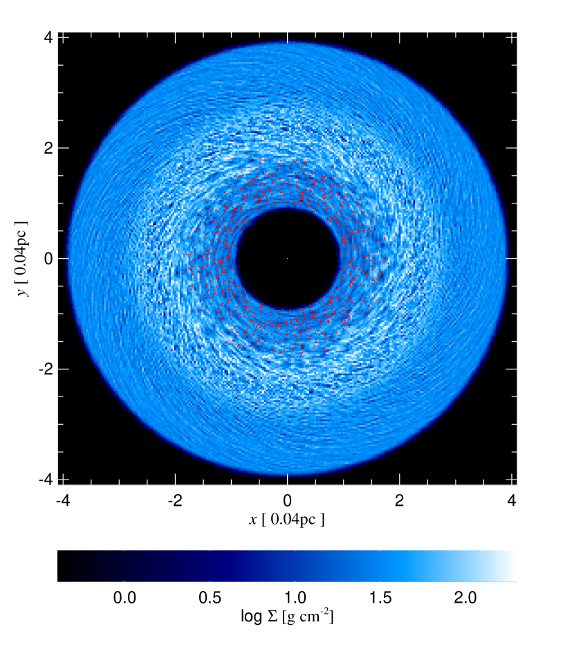
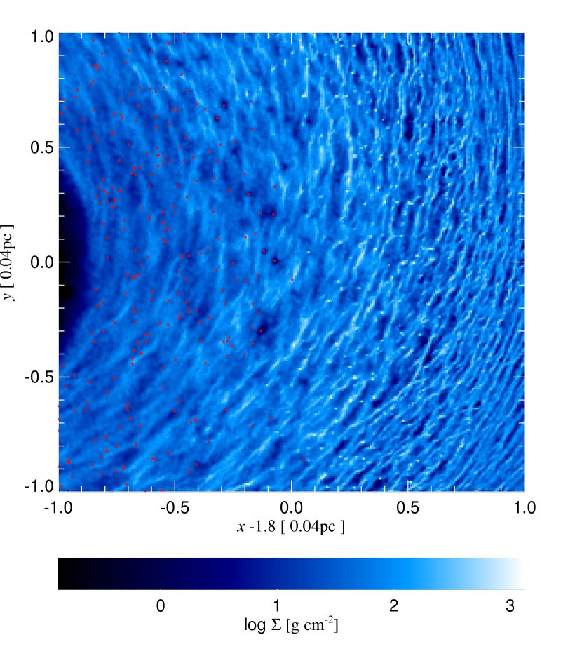
Figure 2: Snapshot of the disc column density at time $t=75$ for test S2 ($\beta=2$). The gas is rotating clockwise in this and all the other figures in this paper. The left hand panel shows the full simulation domain, whereas the right hand one zooms in on a region of the disc centred at $x=1.8$. Stars with masses greater than $3{\,{\rm M}_{\odot}}$ are plotted as red asterisks.

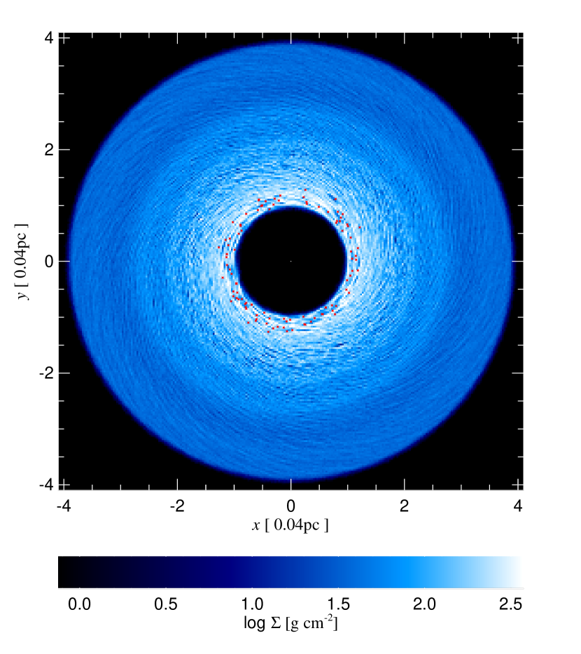
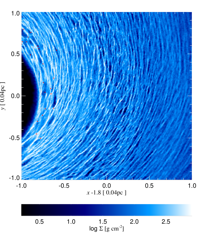
Figure 3: Same as Fig. 2 but for test S3 ($\beta=3$), i.e. for a longer cooling time. Note the smaller number of stars and high density clumps in this test compared with Fig. 2, where the cooling time is shorter.

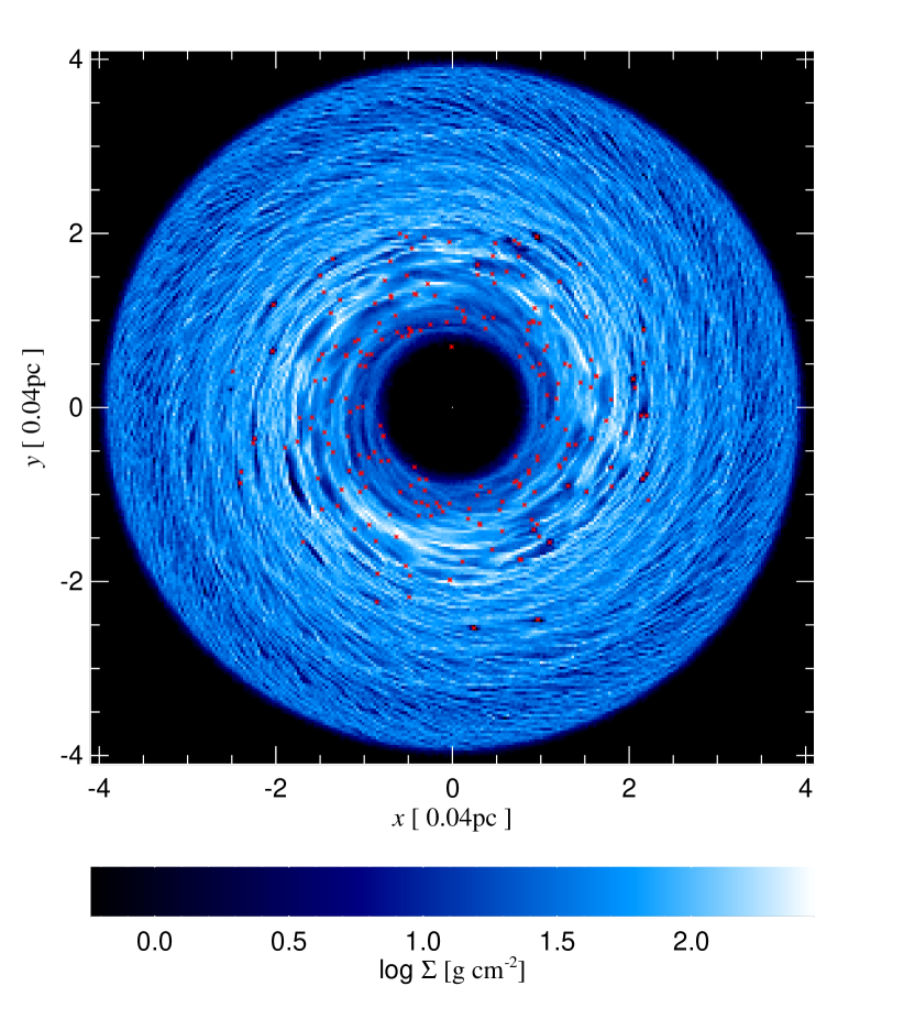
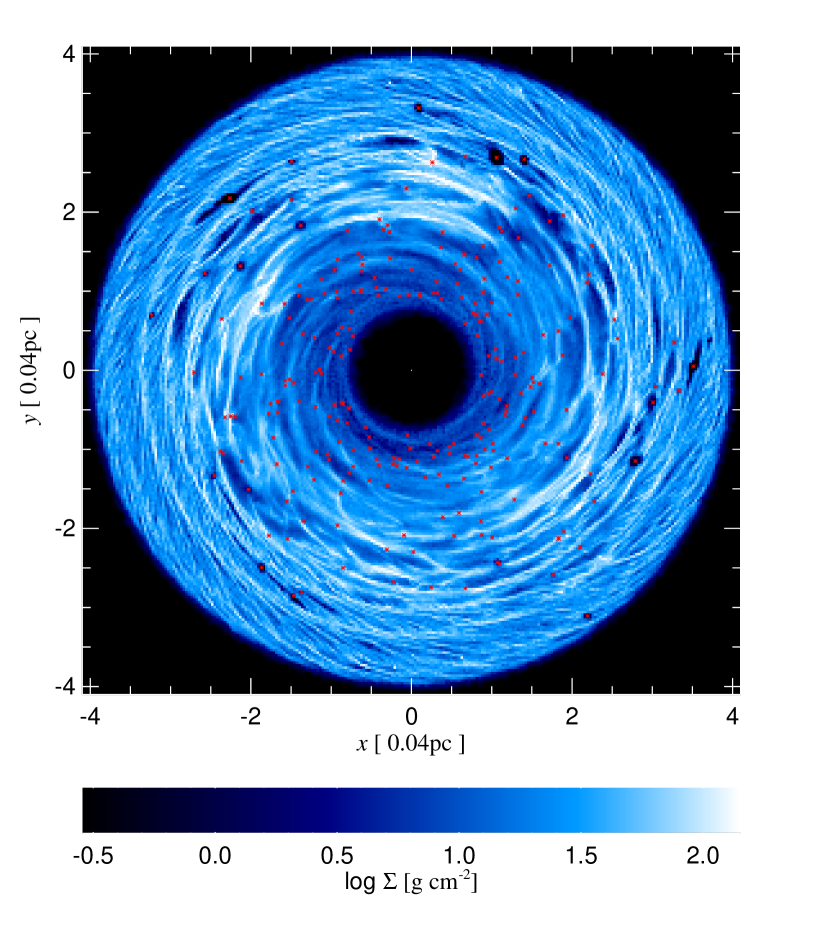
Figure 4: Snapshots of the disc for test S3 at times $t=175$ (left panel) and $t=275$ (right panel). Together with the left panel of Fig. 3, these snapshots trace the gradual depletion of the gaseous disc and the build-up of the stellar disc.

4.1 Evolution of disc vertical thickness

The disc starts off as a razor-thin gaseous disc and evolves into a thicker stellar disc. This behaviour is to be expected. Initially, gas cooling is sufficiently strong, and the disc temperature is regulated to maintain a geometrical thickness of order of $H/R\simeq M_{\rm disc}/{\,{M}_{\rm bh}}$, which is equivalent to having $Q\approx 1$ (e.g., Gammie, 2001). When a good fraction of the gas is turned into stars, however, the rate at which the disc can cool decreases. At the same time, a stellar disc, considered on its own, would thicken with time since stellar orbital energy is transferred into stellar random motions by the normal N-body relaxation processes.

In the intermediate state, when both gas and stars are present in important fractions, disc evolution is not trivial. In the runs described in this section, stars transfer their random energy to the gas via Chandrasekhar’s dynamical friction process (Nayakshin, 2006). The disc swells as time progresses, as can be seen in the two edge-on views of the disc from simulation S2 shown in Fig. 5 . The gaseous disc can thus become thicker than it would have been on its own. However, depending on conditions (i.e. cooling parameter $\beta$, initial total disc mass, mass spectrum of stars), the two discs can be coupled or decoupled. In the latter case the stellar disc has a larger geometrical thickness than the gaseous disc. In such a case the rate at which stars heat the disc is not trivially calculated. This is especially so if stellar radiation, winds and supernovae are taken into account, as stellar energy release above the disc is much less effective in disc heating than it is inside the disc.

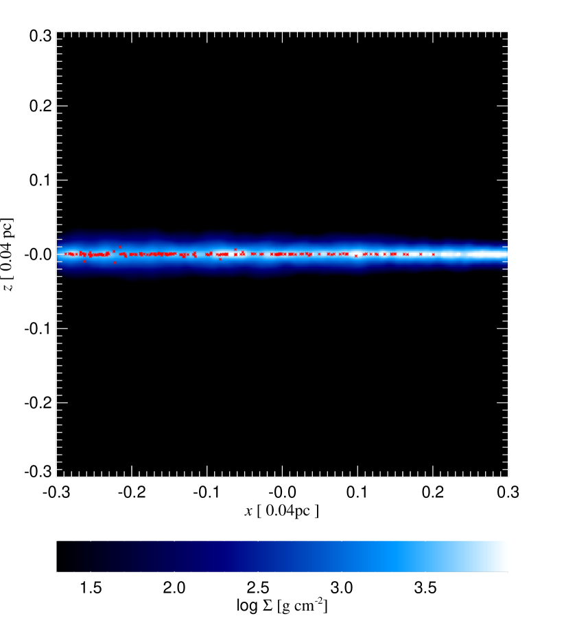
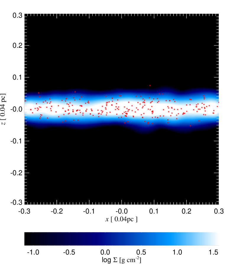
Figure 5: Evolution of the gaseous and stellar disc thicknesses in the test S2. The image is centred at $x=1.3$. The left panel is plotted at time $t=50$, when $\sim 20$% of gas was turned into stars, whereas the right one is for $t=175$, at which point only $\sim 15$% of gas remains in the disc. The disc thickens with time as the remaining gas is not able to provide sufficient damping and cooling of stellar $N$-body heating.

4.2 Fragmentation quenching

Figure 6: Disc fragmentation rate in the tests with $\beta=0.3$ (S1, thick solid), $\beta=2$ (S2, dashed), and $\beta=3$ (S3, thin solid). The shorter the cooling time, the faster disc fragmentation proceeds.

We expect that, following an increase in disc effective temperature and geometrical thickness with time, the vertically averaged density of the disc must drop. The disc may then evolve into a non self-gravitating state as $Q$ increases above unity (see equation 1). Further disc fragmentation should cease. This effect can be noticed in the right hand panel of Fig. 2. Near the inner edge of the disc, there are stars but no high density clumps or filaments implying that the disc is no longer fragmenting in that region.

Figure 6 shows the radius-integrated fragmentation rate of the disc in the simulations with $\beta=0.3$ (run S1, thick solid curve), $\beta=2$ (S2, dashed) and $\beta=3$ (S3, thin solid). The fragmentation rate is defined as the total mass of first cores created per unit time. Not surprisingly, the shorter the cooling time (smaller $\beta$), the more rapid is disc fragmentation. The more vigorous disc fragmentation explains why there are more stars and dense bound gas clumps in Fig. 2 than in Fig. 3 at the same time ($t=75$).

One can also see that the expectation of a decrease of the fragmentation rate with time is borne out. At the peaks of the respective curves, most of the disc mass is still in gaseous form. Therefore, the decline in the fragmentation rate with time is indeed mostly a consequence of a change in the disc state (higher $Q$-parameter) rather than due to the disc running out of gas.

4.3 IMF of the formed stars

It is interesting to compare the distribution functions of stellar masses from our simulations. The end state of our simulations, i.e., when the majority of gas is turned into stars, corresponds to the “initial mass function” (IMF) of a stellar population. Therefore we use this name to refer to our mass distributions. Figure 7 shows the IMF of stars formed in the three simulations S1–S3. Table 1 lists the first two moments of the distribution, i.e., the average mass, $\left<M_{*}\right>$, and $\left<M_{*}^{2}\right>^{1/2}$. It is clear from both the figure and the table, that the longer the cooling time, the more top-heavy (or, equivalently, bottom-light) is the resulting IMF. This outcome is not surprising. As we saw in Section 4.2, fragmentation is fastest for the smallest values of the cooling parameter $\beta$. Further, fragmentation stalls in our models when the stars heat up the disc above $Q=1$ (see Fig. 6). At this point, disc fragmentation stops but accretion onto stars continues. The average mass of a star reached by the time the gas supply is exhausted is roughly inversely proportional to the number of stars at the time the disc fragmentation stalls. As we find many more stars in the tests where fragmentation is quickest, these simulations will also have the least massive IMF.

The shape of stellar IMF formed in our simulations is very different from the IMF in the Solar neighbourhood, which is close to the power-law function of Salpeter (1955). Several authors argued that this might be expected based on theoretical grounds (Morris, 1993; Nayakshin, 2006; Larson, 2006; Levin, 2006). The proportion of massive stars in the stellar population of these discs might be very important for the physics of these discs, e.g., their survival chances against star formation.

Figure 7: Mass function of stars (“IMF”) formed in the simulations with $\beta=0.3$ (S1, solid), $\beta=2$ (S2, dotted), and $\beta=3$ (S3, dashed). The dot-dashed power-law in this and the following plots corresponds to the Salpeter IMF.

5 Sensitivity of results to parameter changes

Due to numerical limitations, our simulations do not include a number of important physical processes. In particular, radiation transfer and chemical processes taking place during collapse of a protostar are dealt with merely via prescriptions. These prescriptions employ parameters which we have tried to set to as physically realistic values as possible. It is important to understand to which degree our results depend on the choices we made for the values of these parameters. Here we describe a selection of tests aimed towards this goal. These tests, labelled E1–E8 in Table 1, were done for slightly different parameters than runs S1–S5. In particular, the inner and outer radii were set to $r_{\rm in}=1$ and $r_{\rm out}=2$, respectively, and the gravitational focusing parameter was chosen to be $f_{m}=1$. The radiative cooling parameter $\beta$ was set to $3$ for all of these tests.

5.1 Maximum accretion rate

We calculate the accretion rate using the Bondi-Hoyle formalism, with the restriction that it is not allowed to exceed the Eddington limit (equations 7 and 9). In principle, excess angular momentum in the gas flow around proto-stars could decrease the accretion rate below our estimates. To explore possible changes in the results, simulations E1 and E3 differed only by the maximum accretion rate allowed, with $1$ and $0.1$ times the Eddington limit, respectively.

The resulting IMFs of these two runs are shown in Fig. 8, along with the IMF for test S3, which was already presented in Fig 7. Comparing the solid curve (simulation E1) with the dashed curve (S3), we see that changes in $r_{\rm out}$, $A_{\rm col}$ and $f_{m}$ did influence the IMF, making it less top-heavy. The main effect stems from the reduction in the value of the gravitational focusing parameter, $f_{m}$. Fewer mergers imply that the final average stellar mass is smaller.

Comparing the runs E1 and E3, one notices that while the IMFs of the two tests are similar at the high mass end, around the peak in the curves, there is a larger discrepancy at the low mass end. The largest difference in the IMFs occurs at around the critical mass, $M_{\rm crit}=0.1{\,{\rm M}_{\odot}}$. The differences are nevertheless not as large as one could expect given an order of magnitude change in the maximum accretion rate. We interpret these results as follows. A star is first born as a low mass star in our simulations, and it then gains mass by either accretion or mergers with the first cores. If the maximum possible accretion rate onto the star is high, it “cleans out” its immediate surroundings of gas, and gains most of its mass by accretion. On the other hand, if the accretion rate is capped at lower values, as in the run E3, then gas gravitationally captured by the star will first settle into a small scale disc around the star. This disc is somewhat smaller than the Hill’s radius $R_{\rm H}=R(M_{*}/3M_{\rm BH})^{1/3}\approx 0.01R$ for the star of mass $M_{*}=10{\,{\rm M}_{\odot}}$. The density in that disc will often exceed the critical density for star formation, and hence new first cores will be introduced in close proximity to the star. These cores then mostly and relatively quickly merge with the star. Because the rate of gas capture from the larger disc (the Hill or the Bondi rate, e.g., Goodman & Tan, 2004; Nayakshin & Cuadra, 2005) is controlled by the total mass inside the Hill radius, the rate at which the dominant star inside the Hill sphere is growing is comparable. The end result (the IMF for massive stars) is then similar, regardless of whether the captured gas was directly accreted or first turned into fluffy proto-stars (the first cores) and then accreted.

Another difference between the results of the runs E1 and E3 is the longer disc life-time, $t_{\rm half}$, for the former simulation for rather obvious reasons.

Figure 8: IMF from the simulations with two different maximum allowed accretion rates (see Section 5.1), i.e., 0.1 times the Eddington rate (E3 in Table 1; dotted curve) and the Eddington rate (E1; solid). These curves are compared with the IMF from simulation S3 (dashed).

5.2 Critical collapse density

Our fragmentation criterium is controlled by two parameters, $\rho_{0}$ and $A_{\rm col}$ (equation 3). The default values for these parameters are $\rho_{0}=5\times 10^{-11}$ g cm^-3, and $A_{\rm col}=60$. These values were used in run E3. The simulations E2, E3a and E4 are completely analogous to the run E3 except for the two parameters controlling the fragmentation. In E2, the fragmentation density threshold is drastically relaxed, with $\rho_{0}=5\times 10^{-12}$ g cm^-3 and $A_{\rm col}=9$. In run E3a, $\rho_{0}=5\times 10^{-12}$ g cm^-3, but $A_{\rm col}=60$, as in E3. Finally, in the run E4 we used $\rho_{0}=5\times 10^{-11}$ g cm^-3, and $A_{\rm col}=300$.

Figure 9 shows the resulting mass function for the stars formed in these four tests. Evidently, a significant relaxation of the fragmentation criteria resulted in very large changes in the IMF at its the low mass end. The high mass end is not so strongly affected. In fact, the IMF of the tests E3 and E4 are almost identical, implying that the results become independent of the value of the critical collapse density (equation 3) when it is chosen large enough.

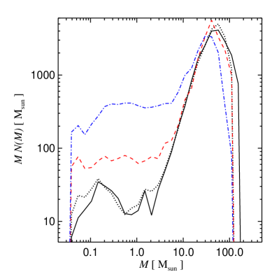
Figure 9: IMF of runs E2, E3, E3a and E4 (blue dash-dotted, red dashed, dotted and solid curves, respectively). The simulations differ by the value of the critical collapse density (see Section 5.2 for details).

5.3 First core size

Runs E3 and E5 are different only in the size of the first cores, $R_{\rm core}$ (see Table 1). Figure 10 demonstrates that the IMF of the simulations is remarkably similar at the high mass end, where it contains almost all of the stellar mass. At the low mass end, however, simulation E5 has significantly more mass than E3. Clearly, the smaller first core radius $R_{\rm core}$ permits fewer mergers and slower growth of first cores by accretion. The exact value of $R_{\rm core}$ is hence important for the low-mass end of the IMF.

Figure 10: Comparison of the IMFs of runs E3 (solid) and E5 (dotted). The simulations have a different “first core” radius parameter, $R_{\rm core}=10^{14}$ and $3\times 10^{13}$ cm, for E3 and E5, respectively. See text in Section 5.3 and Table 1 for details.

5.4 SPH particle mass

The simulations E6–E8 had identical parameter settings but used different initial SPH particle numbers to test the sensitivity of the results on the SPH mass resolution. Figure 11 shows the IMF from these tests. Clearly, there is a significant difference between run E6 (solid; 1 million SPH particles) and the two others, E7 (dotted; 2 million) and E8 (dashed; 4 million). There is a far smaller difference between the two runs with the highest resolution, though, suggesting that the results are reasonably close to full convergence. Given other uncertainties of the runs, e.g., the exact value of the parameter $R_{\rm core}$ and the cooling parameter $\beta$, etc., it seems sufficient to have an SPH mass resolution at the level of the run E7, which has $m_{\rm sph}=0.02{\,{\rm M}_{\odot}}$. Note that except for the simulations E6 and E7, all the other runs presented here used $m_{\rm sph}=0.01{\,{\rm M}_{\odot}}$, as in the test E8.

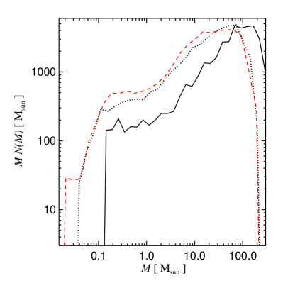
Figure 11: IMF of runs E6–E8. The simulations differ in the initial number of SPH particles used. In particular, $N_{\rm sph}=1$, 2 and $4\times 10^{6}$ for E6, E7 and E8, respectively.

6 IMF and feedback

Nayakshin (2006) suggested that the luminosity of the young stars which accrete gas from within a star-forming disc is sufficient to heat up the disc, increasing the Toomre (1964) $Q$-parameter of the disc above unity and hence making the disc stable to further fragmentation. Nayakshin (2006) also suggested that this will lead to a top-heavy IMF for stars born in such marginally unstable self-gravitating discs. To test these ideas, we ran two additional simulations that had thermal accretion feedback included. The feedback is implemented in the same way as in Springel et al. (2005), with a parameter $0\leq F\leq 1$ introduced to quantify the fraction of the accretion luminosity that is fed back as heat into the surrounding gas. The accretion luminosity of course depends on the accretion rate onto the star (equation 8). The feedback luminosity, $FL_{\rm acc}$, is spread over the SPH neighbours of the accreting star according to their weight in the SPH kernel.

Our two test simulations F1 and F2 had feedback parameters of 0.01 and 0.5, respectively, and are otherwise identical to the run E3, which had $F=0$. One notices right away from Table 1 that the disc lifetime $t_{\rm half}$ becomes longer for the tests with feedback compared with the test E3. In particular, even for F1 with $F=0.01$, the disc lifetime is almost twice larger than for E3. The test F2 in fact could not be ran until “completion”, i.e. until most of the gas turned into stars, as star formation was severely inhibited in that test. At the end of the simulation, after $10^{3}$ time units, the disc lost only about 10% of its mass. We hence could only estimate that $t_{\rm half}$ will be around $10^{4}$ time units. Therefore, the expectation of a stalling of star formation is confirmed in our simulations with the large feedback parameter $F$. However, one has to note that in a more sophisticated approach the disc cooling time needs to be determined self-consistently, whereas we here kept it constant artificially.

The IMFs of the runs F1 and F2 are compared to that of the run E3 in Figure 12. The IMF of the low feedback parameter case, F1, is biased towards massive stars slightly more than that of the simulation E3, providing some support for the predictions of Nayakshin (2006). However, simulation F2 has not been run for long enough to produce a meaningful stellar mass function. In perspective, we suspect that the constant cooling time model is a poor approximation especially when stellar feedback is explored. We shall develop a more realistic cooling model to test the influence of feedback on the disc evolution in the future.

Figure 12: Mass function of stars (“IMF”) formed in the simulations without (solid, run E3) and with feedback. The dashed curve is for run F1, $F=0.01$, whereas the dotted one is for F2, $F=0.5$. Note that in simulation F2, only $\sim 200{\,{\rm M}_{\odot}}$ of stars were formed by the end of the simulation. See text in Section 6 for details.

7 Elliptical orbits

One interesting question raised by the observations of young stars in the central parsec of our Galaxy is that there is apparently a population of young stars on orbits that are quite eccentric (eccentricities of these stars are of the order of 0.7; see Paumard et al., 2006). The two-body relaxation time scale is as long as $\sim 10^{9}$ years at this location (Freitag et al., 2006), so if the origin of these stars lies in in situ star formation, such large eccentricities could not be built up from initial circular orbits (Alexander et al., 2006); consequently their initial orbits should have been eccentric.

To examine whether stars can form in an eccentric gaseous disc or a stream, we set up an additional test that is identical to simulation E1, except for the initial conditions. In this run, designated as “Ecc” in Table 1, the initial gas configuration is that of a disc segment characterized by $4\leq R\leq 7$ and azimuthal angle $0\leq\phi\leq\pi/4$. Further, instead of placing the gas on Keplerian circular orbits with $v=v_{\rm K}(R)=\Omega(R)R$, we decreased the gas velocity to $v=0.7v_{\rm K}(R)$ while keeping its direction perpendicular to its position vector and in the plane of the gas, as in a circular disc. These initial conditions are artificial, i.e. unlikely reached in a realistic infall of a gas cloud into the inner parsec of the Galaxy. However they allow us to test star formation in an eccentric gas disc under simple and controlled conditions.

In addition, we also introduced in this simulation a fixed spherical potential of the older stellar cusp as deduced observationally by Genzel et al. (2003). The total stellar mass of this cusp within the region being simulated is about $\sim 10$% of the mass of Sgr A^∗, i.e. small but not negligible.

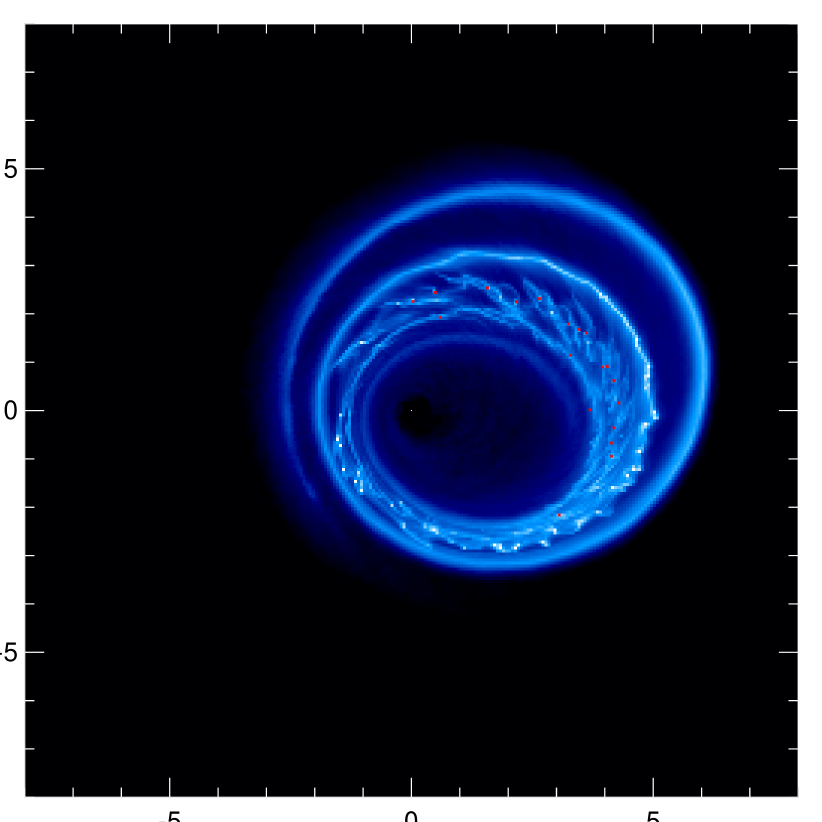
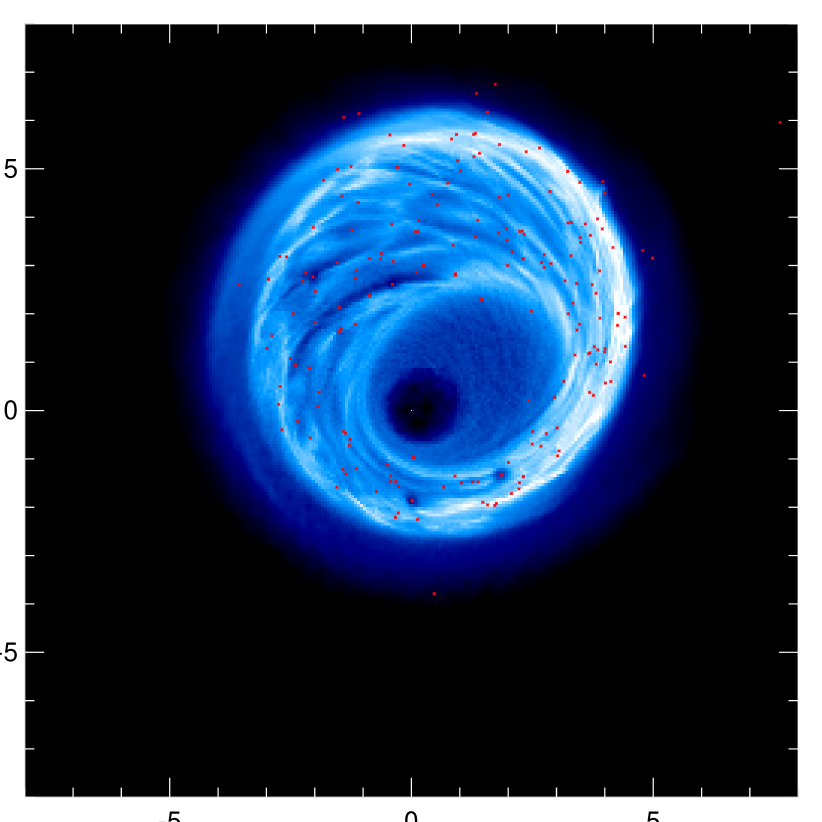
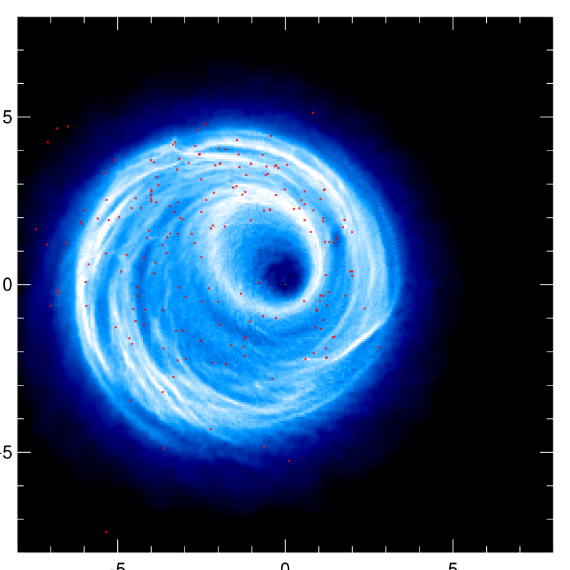
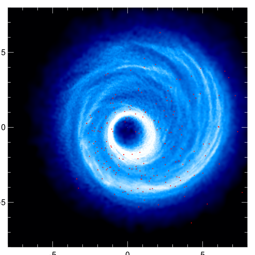
Figure 13: Evolution of the eccentric disc simulation at times corresponding to $t=150$, $450$, $1000$, and $2000$, from left to right and top to bottom. Initially, the disc segment is tidally sheared into an eccentric spiral. While precessing, the spiral forms an eccentric disc. Outer and inner edges of the disc precess at different rates which leads to shocks and circularization of gas orbits. During the simulation, the outer ring of gas makes about 30 rotations and precesses around one full circle.

Figure 13 presents several snapshots of the surface density for test Ecc, along with stars more massive than 3 ${\,{\rm M}_{\odot}}$. Initially the disc segment is torn into an eccentric spiral that makes a few rotations around Sgr A^∗. The spiral develops kinks (which would be essentially parts of spiral arms in a circular gas disc) that run at an angle to the gas spiral. Stars are born within these kinks, in orbits with eccentricities $\sim 0.5$, similar to the original gas orbits. The process differs from the results of Sanders (1998), who simulated the formation of young Galactic Centre stars on elliptical orbits in a sticky-particle approach. In that approach it was found that star formation occured in shocks due to self-collisions of the stream. It is possible that such a shock-mediated star formation would also occur in our model if gas was allowed to cool much faster than the local dynamical time.

Due to the non-Keplerian potential in this test, gas and stellar orbits precess. The precession rate is different at different radii, and therefore gas orbits become mixed and somewhat circularized over time. This is most clearly seen in the last snapshot (lower right) in Fig. 13, where an inner, only mildly eccentric gaseous ring is present.

The simulation Ecc was run for twice longer than our usual $10^{3}$ time units. Nevertheless, at the end of the simulation only $\sim 30$% of gas was turned into stars. We hence estimate the disc half-life time $t_{\rm half}$ to be around 3000 time units. This is $\sim 35$ times longer than that of the corresponding simulation E1 with circular orbits. While some of the difference is simply due to a longer orbital time at the location of the gas in test Ecc, a fair fraction of the difference is due to a comparatively slower star formation. This is not altogether surprising, as gas is heated due to shocks in the eccentric, precessing disc of simulation Ecc.

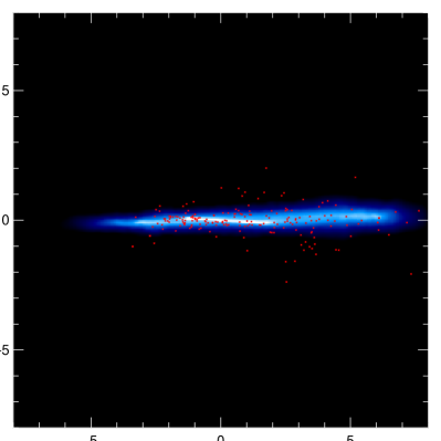
Figure 14: Edge-on column density and stellar positions for the last of the snapshots from Fig. 13. Note that the stellar disc is much thicker than the gaseous disc.

Figure 14 presents an edge-on view of the column density of the disc and stellar positions at the end of the run Ecc. It is quite noticeable that the stellar disc is much thicker than the gaseous disc. While it is difficult to pinpoint the exact reason for this high geometrical thickness, it is most likely due to interactions between stars (e.g., Nayakshin & Cuadra, 2005; Alexander et al., 2006), which can be substantial given that this simulation has been run for over $10^{5}$ years. Disruptions of gas–star clumps at their orbits’ pericentres or during collisions with each other in the disc could also be important.

8 in situ formation of “mini star clusters”

Several authors speculated that self-gravitating AGN discs can form very massive objects. Goodman & Tan (2004) argued that massive stars formed in such discs will continue to accrete until they reach the “isolation” mass, $M_{\rm i}\simeq M_{d}^{3/2}M_{\rm BH}^{-1/2}$,

$$M_{i}\approx 550{\,{\rm M}_{\odot}}\;\left[\frac{M_{d}}{10^{4}{\,{\rm M}_{\odot}}}\right]^{3/2}\left[\frac{3\times 10^{6}{\,{\rm M}_{\odot}}}{M_{\rm BH}}\right]^{1/2}\;.$$ (12)

Such a super-massive star would presumably grow via accretion from a gas disc around it. The linear sizes of the disc would be of the order of the Hill radius of the star, $R_{\rm H}=R(M_{\rm i}/3M_{\rm BH})^{1/3}$. The disc may become quite massive, and fragment further. In this way systems more complicated than a single massive star can be formed. It is not impossible that the compact star cluster IRS13E, which orbits Sgr A^∗ uncomfortably close, was formed in this way (Milosavljević & Loeb, 2004; Nayakshin & Cuadra, 2005; Levin, 2006).

We searched for such massive bound systems containing many stars in the results of our simulations. While we did find many binaries of massive stars, nothing on the scale of the isolation mass was present. In terms of physical effects that could limit the growth of such groups, a too rapid disc fragmentation is the most likely one. Namely, for the smaller value of the cooling parameter $\beta$, the disc fragments quickly into too many stars that then compete for the gas. No clear “winners” emerge, as can be seen from the shape of the IMF, which rolls over very quickly at the higher mass end (see Fig. 7).

For longer cooling times, i.e., $\beta\lower 2.15277pt\hbox{$\;\buildrel>\over{\sim}\;$}1$, disc fragmentation is less vigorous, creating fewer stars, and leading to a more top-heavy IMF. In this case, while the gaseous mass is still comparable to the stellar mass in the simulations, we did find many binaries and multiple systems, some containing up to 6 stars. However, closer to the end of these simulations, when the gas supply was exhausted, only tightly bound binaries remained. There seem to be two reasons for this. Firstly, while the system is still gas-rich, collisions between “mini star clusters” take place. The collisions tend to unbind the systems (since $\beta>1$). A few examples of this could be seen directly in videos of the time evolution of the simulations produced from the snapshots. Secondly, when most of the gas is exhausted, individual multiple systems are likely to evaporate the less massive components in favour of tightening the most massive binary.

These results could in principle simply mean that we do not have a sufficient time resolution to integrate small scale dynamics of stars in these mini star clusters. To check this, we have ran an additional simulation, identical to the run S2, but in which the time step criterium was 2 times more stringent. In this simulation, not presented in the Table 1, individual particle time steps were on average half of what they were in S2. The result was very similar in terms of the IMF (i.e. the average stellar mass and the average stellar mass squared were different by $\sim 3$% and $10$% only). However, we did find a $\sim 50\%$ increase in the number of stars with several close neighboors. However, again, no group was even remotely close to the isolation mass scale. The largest group contained four neighboors. While this issue requires further numerical work, we believe that the absense of massive densely packed stellar groups is not a numerical artefact.

Nevertheless, independently of the precision with which the numerical integration is performed, the results might also strongly depend on the gas cooling physics. A more careful treatment of gas cooling physics is needed in order to test the model of in situ formation of IRS13E more thoroughly.

9 Conclusions

In this paper, we presented some of our first attempts to simulate star formation in an accretion disc around Sgr A^∗in the low disc mass case. Since the relevant physics is only weakly dependent on the mass of the SMBH (Goodman, 2003), we expect that the results are relevant to more massive SMBHs as well. On the technical side, in our numerical method we used a locally constant cooling time prescription, and we allowed for a finite collapse time of stellar “first cores” and their mergers (Sections 2 and 3). We limited the accretion rate of stars to a fraction of the Eddington limit. Our simulations verified that the code reproduces disc fragmentation in agreement with previous analytical and numerical work (Section 2.3). We also tested the dependence of the results on some of the plausible parameter choices (Section 5 and Table 1).

The scientific results of our work can be summarized as follows:

• Qualitatively, star formation in marginally self-gravitating discs, i.e. those that have cooling times just short enough to fragment, results in a top-heavy IMF. This is due to the suppression of fragmentation by disc heating either through N-body effects or feedback from the accretion luminosity. Mergers between first cores and gas accretion lead to a rapid growth of existing stars. Quantitatively, the IMF of our simulations does depend on physics that we do not completely resolve and which we model through several free parameters (see Table 1).

• Without feedback, star formation is a very rapid process (unless cooling is inefficient, of course). As gas is bound to Sgr A^∗, nothing escapes from the star forming region, and essentially all of the gas in the disc is turned into stars.

• Due to point 2, our models completely fail to feed the central AGN. Even the longest “living” gas disc in our runs (test F2 with feedback) would all be drained into young stars after about $10^{6}$ years, which is far too short compared with the normal timescale of feeding Sgr A^∗ through viscous angular momentum transfer (e.g., Nayakshin & Cuadra, 2005). Modelling of higher mass discs is needed to establish whether star formation feedback in such discs could hold off the disc’s demise due to star formation in favour of AGN accretion.

• Discs more massive than marginally self-gravitating discs can be modelled in our approach with a small cooling time parameter, $\beta\ll 1$. Without stellar feedback, such discs undergo a very rapid gravitational collapse. This leads to an IMF dominated by low mass stars. See point 5 below, however.

• We have explored two limiting cases of marginally self-gravitating discs with thermal feedback. Putting even a small fraction of the stellar accretion luminosity back into the disc significantly increases the disc lifetime, that is, it slows down star formation. A more sophisticated numerical treatment of heating/cooling is necessary to test whether the IMF of such discs will become top heavy, as predicted.

• We also simulated star formation in an eccentric stream of gas in the gravitational potential of Sgr A^∗ and the surrounding stellar cusp. The gas stream precesses, self-collides and forms an eccentric disc. Massive stars in eccentric orbits are readily formed in the simulation. Tidal shearing and shocks in the eccentric case do not prevent collapse, though they do increase the lifetime of the gaseous disc.

• None of the simulations formed an object similar to IRS13E, a bound “mini star cluster” in the GC. While more careful modelling is needed to confirm the result, it is suggestive of a formation mechanism for this object different from the in situ star formation in the disc.

We thank Giuseppe Lodato for detailed comments on the paper.

Simulation	$\beta^{\,a}$	$F^{\,b}$	$N_{\rm sph}$,	Disc radial	$M_{\rm disc}$,	$A_{\rm col}^{\,c}$	Max. accre-	$R_{\rm core}$	$f_{\rm m}^{\,e}$	$t_{\rm half}^{f}$	$M_{*}$,	$\sqrt{M_{*}^{2}}$,
name and purpose			$10^{6}$	extent	${\,{\rm M}_{\odot}}$		tion rated	$10^{14}$ cm			${\,{\rm M}_{\odot}}$	${\,{\rm M}_{\odot}}$
fragmentation study
S1	0.3	0	4	$1-4$	$3\times 10^{4}$	30	1	1	3	$10.5$	$0.35$	$0.43$
S2	2.	0	4	$1-4$	$3\times 10^{4}$	30	1	1	3	$88$	$2.6$	$3.7$
S3	3.	0	4	$1-4$	$3\times 10^{4}$	30	1	1	3	$230$	$59.6$	$76.3$
S4	4.5	0	4	$1-4$	$3\times 10^{4}$	30	1	1	3	–	–	–
S5	6.	0	4	$1-4$	$3\times 10^{4}$	30	1	1	3	–	–	–
Maximum $\dot{M}_{*}$
E1	3.	0	2	$1-2$	$2\times 10^{4}$	60	1	1	1	86	9.9	17.0
E3	3.	0	2	$1-2$	$2\times 10^{4}$	60	0.1	1	1	240	5.7	15.5
Critical density
E2	3.	0	2	$1-2$	$2\times 10^{4}$	9	0.1	1	1	235	0.55	3.3
E3	3.	0	2	$1-2$	$2\times 10^{4}$	60	0.1	1	1	240	5.7	15.5
E3a	3.	0	2	$1-2$	$2\times 10^{4}$	60	0.1	1	1	240	1.9	8.3
E4	3.	0	2	$1-2$	$2\times 10^{4}$	300	0.1	1	1	245	8.0	19.2
First core size
E3	3.	0	2	$1-2$	$2\times 10^{4}$	60	0.1	1	1	240	5.7	15.5
E5	3.	0	2	$1-2$	$2\times 10^{4}$	60	0.1	0.3	1	240	0.6	4.7
Resolution study
E6	3.	0	1	$1-2$	$4\times 10^{4}$	60	1	1	1	43	5.3	20.4
E7	3.	0	2	$1-2$	$4\times 10^{4}$	60	1	1	1	44	2.0	8.1
E8	3.	0	4	$1-2$	$4\times 10^{4}$	60	1	1	1	44	1.5	6.5
feedback importance
F1	3.	0.01	2	$1-2$	$2\times 10^{4}$	60	0.1	1	1	$400$	5.4	17.4
F2	3.	0.5	2	$1-2$	$2\times 10^{4}$	60	0.1	1	1	$\sim 10^{4}$	(?)	(?)
Eccentric orbits
Ecc	3.	0	2	$\sim 1-7$	$2\times 10^{4}$	60	1	1	1	$\approx 3000$	9.9	17.0

Table 1: Description of simulations performed in the paper. Some of the run are printed several times in the table to allow an easier comparison between the tests grouped together. Notes:

^a Cooling parameter introduced in Section 2.2.

^b Feedback parameter, the fraction of stellar accretion energy fed back into the disc (Section 6).

^c Collapse over-density parameter (Section 2.1)

^d The maximum accretion rate of sink particles in units of their Eddington accretion rate (see Sections 5.1 & 3.3).

^e Gravitational focusing parameter for mergers of first cores (Section 3.1)

^f Time scale for the gaseous mass in the disc to drop by half.

References

- Alexander et al. (2006) Alexander R. D., Begelman M. C., Armitage P. J., 2006, ArXiv Astrophysics e-prints
- Bate et al. (1995) Bate M. R., Bonnell I. A., Price N. M., 1995, MNRAS, 277, 362
- Bertin & Lodato (1999) Bertin G., Lodato G., 1999, A&A, 350, 694
- Collin & Zahn (1999) Collin S., Zahn J., 1999, A&A, 344, 433
- Demircan & Kahraman (1991) Demircan O., Kahraman G., 1991, Astrophysics and Space Science, 181, 313
- Ferrarese et al. (2006) Ferrarese L., Côté P., Dalla Bontà E., et al., 2006, ApJL, 644, L21
- Freitag et al. (2006) Freitag M., Amaro-Seoane P., Kalogera V., 2006, ApJ, 649, 91
- Gammie (2001) Gammie C. F., 2001, ApJ, 553, 174
- Genzel et al. (2003) Genzel R., Schödel R., Ott T., et al., 2003, ApJ, 594, 812
- Goldreich & Tremaine (1980) Goldreich P., Tremaine S., 1980, ApJ, 241, 425
- Goodman (2003) Goodman J., 2003, MNRAS, 339, 937
- Goodman & Tan (2004) Goodman J., Tan J. C., 2004, ApJ, 608, 108
- Gorda & Svechnikov (1998) Gorda S. Y., Svechnikov M. A., 1998, Astronomy Reports, 42, 793
- Kolykhalov & Sunyaev (1980) Kolykhalov P. I., Sunyaev R. A., 1980, Soviet Astron. Lett., 6, 357
- Larson (1969) Larson R. B., 1969, MNRAS, 145, 271
- Larson (2006) Larson R. B., 2006, in Revista Mexicana de Astronomia y Astrofisica Conference Series, 55–59
- Levin (2006) Levin Y., 2006, ArXiv Astrophysics e-prints,astro-ph/0603583
- Levin & Beloborodov (2003) Levin Y., Beloborodov A. M., 2003, ApJ, 590, L33
- Lin & Pringle (1987) Lin D. N. C., Pringle J. E., 1987, MNRAS, 225, 607
- Masunaga et al. (1998) Masunaga H., Miyama S. M., Inutsuka S.-I., 1998, ApJ, 495, 346
- Milosavljević & Loeb (2004) Milosavljević M., Loeb A., 2004, ApJL, 604, L45
- Morris (1993) Morris M., 1993, ApJ, 408, 496
- Nayakshin (2004) Nayakshin S., 2004, MNRAS, 352, 1028
- Nayakshin (2006) Nayakshin S., 2006, MNRAS, 372, 143
- Nayakshin & Cuadra (2005) Nayakshin S., Cuadra J., 2005, A&A, 437, 437
- Nayakshin et al. (2006) Nayakshin S., Dehnen W., Cuadra J., Genzel R., 2006, MNRAS, 366, 1410
- Nayakshin & Sunyaev (2005) Nayakshin S., Sunyaev R., 2005, MNRAS, 364, L23
- Paczyński (1978) Paczyński B., 1978, Acta Astron., 28, 91
- Paumard et al. (2005) Paumard T., Genzel R., Eisenhauer F., Ott T., Trippe S., 2005, submitted to ApJ
- Paumard et al. (2006) Paumard T., Genzel R., Martins F., et al., 2006, ApJ, 643, 1011
- Rafikov (2005) Rafikov R. R., 2005, ApJL, 621, L69
- Rice et al. (2005) Rice W. K. M., Lodato G., Armitage P. J., 2005, MNRAS, 364, L56
- Salpeter (1955) Salpeter E. E., 1955, ApJ, 121, 161
- Sanders (1998) Sanders R. H., 1998, MNRAS, 294, 35
- Schödel et al. (2002) Schödel R., Ott T., Genzel R., et al., 2002, Nature, 419, 694
- Schödel et al. (2005) Schödel R., Eckart A., Iserlohe C., Genzel R., Ott T., 2005, ApJL, 625, L111
- Shakura & Sunyaev (1973) Shakura N. I., Sunyaev R. A., 1973, A&A, 24, 337
- Shlosman & Begelman (1989) Shlosman I., Begelman M. C., 1989, ApJ, 341, 685
- Silk (1977) Silk J., 1977, ApJ, 214, 152
- Sirko & Goodman (2003) Sirko E., Goodman J., 2003, MNRAS, 341, 501
- Springel (2005) Springel V., 2005, MNRAS, 364, 1105
- Springel et al. (2005) Springel V., Di Matteo T., Hernquist L., 2005, MNRAS, 361, 776
- Springel et al. (2001) Springel V., Yoshida N., White S. D. M., 2001, New Astronomy, 6, 79
- Syer et al. (1991) Syer D., Clarke C. J., Rees M. J., 1991, MNRAS, 250, 505
- Toomre (1964) Toomre A., 1964, ApJ, 139, 1217
- Wehner & Harris (2006) Wehner E. H., Harris W. E., 2006, ApJL, 644, L17
- Yu & Tremaine (2002) Yu Q., Tremaine S., 2002, MNRAS, 335, 965