The effect of spiral arm passages on the evolution of stellar clusters

Abstract

We study the effect of spiral arm passages on the evolution of star clusters on planar and circular orbits around the centres of galaxies. Individual passages with different relative velocity ($V_{\rm drift}$) and arm width are studied using $N$-body simulations. When the ratio of the time it takes the cluster to cross the density wave to the crossing time of stars in the cluster is much smaller than one, the energy gain of stars can be predicted accurately in the impulsive approximation. When this ratio is much larger than one, the cluster is heated adiabatically and the net effect of heating is largely damped. For a given duration of the perturbation, this ratio is smaller for stars in the outer parts of the cluster compared to stars in the inner part. The cluster energy gain due to perturbations of various duration as obtained from our $N$-body simulations is in good agreement with theoretical predictions taking into account the effect of adiabatic damping. Perturbations by the broad stellar component of the spiral arms on a cluster are in the adiabatic regime and, therefore, hardly contribute to the energy gain and mass loss of the cluster. We consider the effect of crossings through the high density shocked gas in the spiral arms, which result in a more impulsive compression of the cluster. The energy injected during each spiral arm passage can exceed the total binding energy of a cluster, but, since most of the energy goes in high velocity escapers from the cluster halo, only relatively little mass is lost. A single perturbation that injects the same amount of energy as the initial (negative) cluster energy causes at most $\sim$40% of the stars to escape. We find that a perturbation that delivers $\sim$10 times the initial cluster energy is needed to completely unbind a cluster in a single passage. The net effect of spiral arm perturbations on the evolution of low mass ($\lesssim 100\,\mbox{${\rm M}_{\odot}$}$) star clusters is more profound than on more massive clusters ($\gtrsim 1000\,\mbox{${\rm M}_{\odot}$}$). This is due to the fact that the crossing time of stars in the latter is shorter, causing a larger fraction of stars to be in the adiabatic regime. The time scale of disruption by subsequent spiral arm perturbations depends strongly on position with respect to the radius of corotation ($R_{\rm CR}$), where $\mbox{$V_{\rm drift}$}=0$. The time between successive encounters scales with $V_{\rm drift}$ as $\mbox{$t_{\rm drift}$}\propto\mbox{$V_{\rm drift}$}^{-1}$ and the energy gain per passage scales as $\Delta E\propto V^{2}_{\rm drift}$. Exactly at $R_{\rm CR}$ passages do not occur, so the time scale of disruption is infinite. The time scale of disruption is shortest at $\sim$0.8-0.9 $R_{\rm CR}$, since there $V_{\rm drift}$ is low. This location can be applicable to the solar neighbourhood. In addition, the four-armed spiral pattern of the Milky Way makes spiral arms contribute more to the disruption of clusters than in a similar but two-armed galaxy. Still, the disruption time due to spiral arm perturbations there is about an order of magnitude higher than what is observed for the solar neighbourhood, making spiral arm perturbations a moderate contributor to the dissolution of open clusters.

1 Introduction

The distinct difference between open and globular clusters has vanished since the discovery of young massive clusters in merging and interacting galaxies (e.g. Holtzman et al. 1992; Whitmore et al. 1999). There is, however, still an evident difference in evolution. Star clusters formed in discs, which in our Galaxy are referred to as open clusters, experience external perturbations by giant molecular clouds (GMCs) and by spiral arms and other disc density perturbations. These are not present in the halo of a galaxy, where most of the globular clusters reside. To understand how cluster populations, such as the open clusters in the solar neighbourhood (Kharchenko et al., 2005) and such as the ones found in spiral galaxies like M51 (Bastian et al., 2005) and NGC 6946 (Larsen et al., 2001), evolve, it is important to understand the effect of these external perturbations.

The number of Galactic open clusters as a function of age shows a lack of old open clusters, first pointed out by Oort (1958). This lack can partially be explained by the rapid fading of clusters with age due to stellar evolution, which makes it harder to observe them at older ages. Still, fading can not explain the difference between the observed and the expected number of old ($\gtrsim 1\,$Gyr) open clusters, implying that a significant fraction must have been destroyed (Wielen 1971; Lamers et al. 2005). In addition to two-body relaxation, clusters in tidal fields dissolve by the combined effect of: A.) Mass loss due to stellar evolution, reducing the mass and hence the binding energy of the cluster; B.) the tidal field of the host galaxy, imposing a tidal boundary, increasing the escape rate of stars; C.) bulge/disc shocks, pushing stars over the tidal boundary and D.) additional perturbations induced by irregularities in the galaxy, such as GMCs and spiral arms. The importance of the first three effects has been studied in detail by many people (for example Chernoff & Weinberg 1990; Gnedin & Ostriker 1997; Gnedin, Lee & Ostriker 1999; Takahashi & Portegies Zwart 2000; Baumgardt & Makino 2003), using different techniques (e.g. Fokker-Planck calculations or $N$-body simulations).

These studies were mainly aimed at understanding the evolution of globular clusters residing in the Galactic halo. The observed short disruption time ($\sim 100\,$Myr) of disc clusters in the grand-design spiral galaxy M51 (Gieles et al., 2005) is an order of magnitude lower than expected from the tidal field of the galaxy (Lamers, Gieles & Portegies Zwart, 2005). Even for clusters in the solar neighbourhood, $N$-body simulations predict disruption times five times longer than observed. These $N$-body simulations, however, ignore the presence of spiral arms (for example Takahashi & Portegies Zwart 2000 and Baumgardt & Makino 2003). In this paper, we study the contribution of spiral density waves to the cluster dissolution time.

Spiral arms are believed to be density waves rotating around the galaxy centre with an angular pattern speed ($\Omega_{\rm p}$) which is independent of the distance $R$ to the galactic centre (see Athanassoula 1984 for a review). The radius at which $\Omega_{\rm p}$ is equal to the angular velocity in the disc ($\Omega(r)=\mbox{$V_{\rm disc}$}/R$, where $V_{\rm disc}$ the circular velocity in the disc) is called the corotation radius ($R_{\rm CR}$). As gas travels through such a density wave, it gets shocked and compressed to five to ten times higher densities (Roberts, 1969). This is observable as narrow sharp dust lanes in optical images of (nearly) face-on spiral galaxies which are far from edge-on.

A cluster on a circular orbit around the centre of the galaxy will, in the inertial frame, have a velocity equal to the circular velocity $V_{\rm disc}$. In the reference frame of the spiral arm, its velocity (hereafter drift velocity, $V_{\rm drift}$) is equal to

$$V_{\rm drift} = \mbox{$V_{\rm disc}$}-\mbox{$\Omega_{\rm p}$}R$$ (1)

$$= \mbox{$V_{\rm disc}$}\left[1-R/\mbox{$R_{\rm CR}$}\right].$$

The absolute value of $V_{\rm drift}$ decreases going from the galaxy centre to $R_{\rm CR}$, where it is zero, and increases again beyond that radius. The time it takes for a cluster to travel from one arm to the next is defined as the drift time: $\mbox{$t_{\rm drift}$}(R)\equiv 2\pi R/(m\,|\mbox{$V_{\rm drift}$}(R)|)$, where $m$ is the number of spiral arms in the galaxy. Thus, near to $R_{\rm CR}$, a cluster experiences few passages but of long duration, while at considerably smaller, or considerably larger radii it undergoes many short-lasting spiral arm passages with high velocity. As it moves from the low density inter-arm region to the high density in the arms, the cluster gets compressed due to tidal forces. These accelerate the cluster stars, some of which may reach the escape velocity and become unbound.

This is comparable to what happens to a globular cluster that crosses the Galactic disc (Ostriker, Spitzer & Chevalier, 1972). There are, however, important qualitative differences between spiral arm perturbations and disc shocks. In particular, globular clusters cross the disc with a velocity almost independent of $R$. On the contrary, the velocity of the cluster with respect to the spiral depends strongly on the distance to the centre. Similarly, the scale-height of a disc is independent of $R$, provided the galaxy is not barred (van der Kruit & Searle, 1981a, b, 1982a, 1982b; de Grijs & van der Kruit, 1996). For spiral arms, on the contrary, it is the angular width of the arm that is roughly independent of radius, so that the linear width of a spiral arm is proportional to the radius.

The passage duration determines the nature of the perturbation of the arm on the cluster. If the time to cross the arm ($T_{\rm cr}$) is much longer than the crossing time of stars in the cluster ($t_{\rm cr}$), the stars can adiabatically adjust to the density increase. When $T_{\rm cr}$ is much shorter than $t_{\rm cr}$, the stars get an impulsive velocity increase due to tidal forces. Stars in the cluster core have a short $t_{\rm cr}$ and, therefore, get adiabatically heated. The boundary between adiabatic and impulsive heating in the cluster is determined by the ratio $t_{\rm cr}$/$T_{\rm cr}$. If this ratio is low, a higher fraction of stars is heated impulsively.

In this paper we study the effect of spiral arm passages on clusters and investigate the importance of relative velocity with respect to the arm. This paper is organised as follows: In Section 2 the physical parameters of spiral arms are derived from observations. Simple analytical estimates of the effects of compressive perturbations are given in Section 3. They are confronted with results of $N$-body simulations in Section 4. In Section 5 the results of the simulations are used to derive cluster mass loss and disruption times due to the spiral arm perturbations. The conclusions are presented in Section 6.

2 Spiral arm parameters

2.1 Stellar arms

Disc clusters are found to have short disruption times both in our Galaxy and in M51. Therefore, we will hereafter consider two fiducial spiral galaxies, one Milky-Way-like – which we will call for brevity Milky Way, or MW – and the other M51-like – which we will call grand design spiral. We will adopt for both a constant rotational velocity of $\mbox{$V_{\rm disc}$}=220\,\mbox{km$\,$s${}^{-1}$}$, that is, we limit ourselves to the regions where their respective rotation curves are flat.

Spiral patterns are present in both young and old populations, as already noted by Zwicky (1955) and later by Schweizer (1976). The old Population II stars in the disc show a broad spiral pattern. In contrary, the young Population I stars, which form preferentially in the spiral arms, show more irregular spiral patterns. Estimates of the arm-interarm density contrast ($\Gamma$) of the stellar population in the disc of M51 were made by Rix & Rieke (1993) and by Gonzalez & Graham (1996), using the $K$-band light as tracer of stellar mass. Their results are in good agreement and show that the maximum value for $\Gamma$ is around $2-3$. Similar values have been found for other grand design spirals (e.g. NGC 4254, see Kranz, Slyz & Rix 2001). We expect our own Galaxy to have smaller values of $\Gamma$. Indeed, Drimmel & Spergel (2001) find a value of $\Gamma\simeq 1.3$ from model comparisons to $K$-band measurements.

M51 has a clear two-armed ($m$ = 2) grand-design spiral, presumably due to the interaction with its companion NGC 5195. The structure of our Galaxy is more complex. It has a bar (see Dehnen 2002 for a review and references therein) and a spiral structure which could rotate with a pattern speed different from that of the bar (Tagger et al., 1987; Sygnet et al., 1988). Drimmel (2000) and Drimmel & Spergel (2001) modelled the COBE-DIRBE data and propose that the old stellar population has a two armed spiral, while the gas and young and stars form a four-armed spiral (for the latter see also Georgelin & Georgelin 1976). Studies in which all components (bar and spirals) have the same pattern speed find that the solar neighbourhood is well beyond corotation (Dehnen, 2000; Fux, 2001), but models allowing for a different pattern speed for the bar and spiral components give a better view of the complex structure in our Galaxy. Bissantz et al. (2003) calculate the gas response to a composite bar plus spiral model and find best agreement for the observations with a pattern speed of $60\,\mbox{km$\,$s${}^{-1}$}\,$kpc^-1 for the bar and $20\,\mbox{km$\,$s${}^{-1}$}\,$kpc^-1 for the spiral. Similar values are found by Martos et al. (2004). This places the solar neighbourhood well beyond the bar corotation, but just within the spiral corotation. With an adopted solar radius of $R_{0}=8.5\,$kpc and the adopted value for $\mbox{$V_{\rm disc}$}=220\,\mbox{km$\,$s${}^{-1}$}$ the solar neighbourhood is at $R\simeq 0.8\,\mbox{$R_{\rm CR}$}$. Compared to the Milky Way, M51 has been modelled very little and no clear-cut value has been given for its pattern speed. Recently, Zimmer, Rand & McGraw (2004) and Egusa, Sofue & Nakanishi (2004) determined the pattern speed of four grand design two-armed spirals and they find values, between 30 and 40 km s^-1 kpc^-1. We adopt $R_{\rm CR}$= 6 kpc, resulting in a pattern speed of $\sim 37\,\mbox{km$\,$s${}^{-1}$\,${\rm kpc}^{-1}$}$.

To further quantify the effect of a spiral-arm passages on the evolution of star clusters, we also need to consider the width of the arms. To enable a quantitative discussion about spiral-arm width, we define $0pt$ as the arm annular full width at half maximum. The typical values of 0pt  measured from optical images of six spiral galaxies by Schweizer (1976), is almost independent of $R$ and $0pt\simeq 20^{\circ}$. Seigar & James (1998) studied $K$-band images of a sample of 45 face-on spiral galaxies and found for two-armed spiral galaxies typical values of $0pt$ between $20^{\circ}$ and $40^{\circ}$. These values are slightly higher than found by Schweizer (1976), probably because the $K$-band is a better tracer of the old stellar populations, for which 0pt is larger. For $0pt=30^{\circ}$, the value of $T_{\rm cr}$ depends on $V_{\rm drift}$ and $R$ as $\mbox{$T_{\rm cr}$}\simeq 0.5R/|\mbox{$V_{\rm drift}$}|$. For the solar neighbourhood $\mbox{$T_{\rm cr}$}\simeq 80\,$Myr. For our M51-like galaxy, the values for $T_{\rm cr}$ at $[0.3/0.5]\times\mbox{$R_{\rm CR}$}$ are $[14,68]\,$Myr. The values for $T_{\rm cr}$ are all higher than the typical $t_{\rm cr}$ of clusters, that is, a few Myrs. Therefore, the stars in the cluster respond adiabatically when the cluster crosses the arm and this crossing does not have the short lasting compressive effect as a galactic disc has on globular clusters.

2.2 Gaseous arms

The gaseous spiral pattern is different from the stellar one. Gas gets shocked in the potential well of the stellar arms, where it gets compressed to up to ten times higher densities (Roberts, 1969). These high gas densities manifest themselves in optical observations of spiral galaxies as thin dust lanes on the leading side of the arm within $R_{\rm CR}$. After the shock, the density decreases exponential-like to a value slightly lower than the mean gas density, as is illustrated in Fig. 1. Such strongly peaked high gas densities act as a compressive perturbation on the cluster (Section 3), which can be compared to disc shocks of globular clusters. The disc crossing is referred to as a shock in that context because of the short duration of the perturbation. That is, the time to cross the disc is much shorter than $t_{\rm cr}$. Since we here also discuss shocks by gas in the arm we avoid confusions and refer to perturbations instead of shocks. In addition, in Section 3 we will show that, due to the variation of $T_{\rm cr}$ with $R$, the perturbations are of highly varying duration.

Besides the higher densities, also the typical values of 0pt of the gaseous spiral arm are much smaller than the one of the stars. Roberts (1969) argues that the width can be calculated by the time scale of formation and evolution of massive stars, that is, a few tens of Myr, since these stars are visible in the optical, so they must have traveled out of the high density dusty environment where they formed. Studies of the molecular spiral arms in M31 and M51 by Nakai et al. (1994) and Nieten et al. (2006), give values of the full-width at half maximum ($W_{1/2}$) of $500\,$pc and $1000\,$pc, respectively. Since these values are close to the resolution of the beam, the sharp peak in density (Fig. 1) is presumably not resolved. Hydrodynamical simulations of barred galaxies revealed narrower density peaks of the gas (see Fig. 11 of Athanassoula 1992), very close to what was predicted by Roberts (1969) and what is shown in Fig. 1. We also measured the width of the dust lane on an optical picture of M51 and the width of the HI on the 8 arcsec resolution map of Rots et al. (1990) and find that they are both compatible with a width of 250 pc. We, therefore, adopt $\mbox{$W_{1/2}$}=250\,$pc for the gaseous arms.

Measurements of the neutral hydrogen content in a sample of spiral galaxies in the Virgo cluster (Cayatte et al., 1994) show that the surface density of HI gas ($\Sigma_{\rm HI}$) within $R\simeq 10\,$kpc in gas rich spirals is nearly constant with $R$ and of the order of $\mbox{$\Sigma_{\rm HI}$}\simeq 10\,\mbox{${\rm M}_{\odot}$}{\rm pc}^{-2}$. A recent study of the Milky Way (Levine, Blitz & Heiles, 2006) gives similar values for $\Sigma_{\rm HI}$ in the solar neighbourhood. Levine et al. (2006) also find that $\Gamma$ is almost independent of $R$. Their measurements of the arm-interarm surface density contrast, combined with the measured vertical compression factor in the spiral arms are consistent with $\Gamma=10$ for the gas.

From $\Sigma_{\rm HI}$ and the vertical scale height of gas ($H_{\rm z}$) we can derive the mean midplane density of HI ($\langle\rho_{\rm HI}\rangle$), since $\mbox{$\langle\rho_{\rm HI}\rangle$}=\mbox{$\Sigma_{\rm HI}$}/2\mbox{$H_{\rm z}$}$, assuming an exponential vertical density distribution. van der Kruit (1988) finds a vertical scale height of $\mbox{$H_{\rm z}$}\simeq 150\,$pc, resulting in $\mbox{$\langle\rho_{\rm HI}\rangle$}\simeq 0.033\,\mbox{${\rm M}_{\odot}$}\,$pc^-3. The peak density ($\rho_{0}$) is then

$$\rho_{0}\simeq\Gamma\,\mbox{$\langle\rho_{\rm HI}\rangle$},$$ (2)

where we assume $\Gamma$ is the ratio of $\rho_{0}$ to $\langle\rho_{\rm HI}\rangle$.

All parameters of spiral arms, used in our models, are summarised in Table 1.

Table 1: Adopted parameters for spiral arms in our fiducial grand design two-armed spiral galaxy and in the Milky Way

	Grand design	Milky Way
$m$	2	4
$\mbox{$V_{\rm disc}$}\,(\mbox{km$\,$s${}^{-1}$})$	220	220
$\Omega_{p}\,(\mbox{km$\,$s${}^{-1}$\,${\rm kpc}^{-1}$})$	36.7	24.5
$R_{\rm CR}$ (kpc)	6	9
$0pt$(stars)	$30^{\circ}$	$15^{\circ}$
$W_{1/2}$(gas) (pc)	250	250
$\Gamma_{\rm stars}$	2-3	$<2$
$\Gamma_{\rm gas}$	10	10
$\langle\rho_{\rm HI}\rangle$ (${\rm M}_{\odot}$ pc-3)	0.033	0.033

2.3 Potential-density relations for the arms

The density of gas along the orbit of the cluster has a sharp rise at the point where the shock occurs and an exponential-like decrease after the shock (see our Fig. 1 and Fig. 5 of Roberts 1969). In reality, the density increase is bit smoother than shown in Fig. 1. It is hard, if not impossible, to derive a suitable potential that describes a realistic density function. Therefore, we assume for simplicity a one-dimensional density perturbation of Gaussian form

$$\rho(Y)=\rho_{0}\,\exp(-Y^{2}/H^{2}),$$ (3)

where $H$ is the scale length and $Y$ is the azimuthal distance. In Section 3 we show that for an impulsive perturbation the compressive tidal forces on the cluster scale with the integral of $\rho(Y)$ with respect to $Y$, where $Y$ is the direction of motion of the cluster. A Gaussian function with a integral equal to that of an exponential function has the same compressive effect on the cluster. We emphasise that this is only true when for both perturbations hold that they are impulsive. In practise, this implies that the majority of the surface should be contained within the same $Y$ extent for both functions. That is, a very broad gaussian with the same surface as a very peaked gaussian will have a different effect on the cluster, because the broad gaussian will heat the cluster adiabatically, while the peaked gaussian will heat the cluster impulsively. For the exponential function $\rho(Y)=\rho_{0}\,\exp(-Y/\mbox{$W_{1/2}$})$, for $Y>0$, and the Gaussian function of equation (3), the surfaces are equal when $H=\mbox{$W_{1/2}$}/\sqrt{\pi}$. With Table 1 we thus find that $H\simeq 150\,$pc for the gaseous arms.

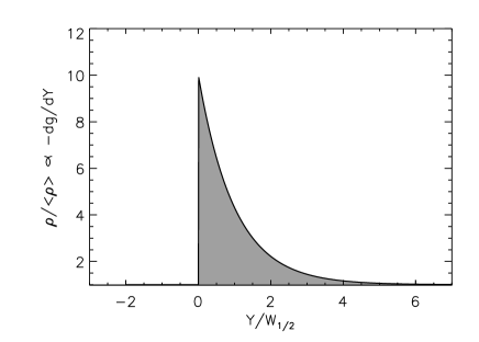
Figure 1: Schematic illustration of the gas density along azimuthal trajectories through a spiral arm, where the gas travels from left to right in this figure. The grey shaded area is the gas density predicted by Roberts (1969). When the scale length of a Gaussian function ($H$) is $1/\sqrt{\pi}$ times the scale length of the exponential function ($W_{1/2}$), the areas under the two curves are the same.

By using Poisson’s law and equation (3) we can derive the related potential along the trajectory of the cluster

$$\phi(Y)=2\pi G\rho_{0}H\left[\sqrt{\pi}Y\mbox{${\rm erf}$}(Y/H)+H\exp(-Y^{2}/H^{2})\right],$$ (4)

where $G$ is the gravitational constant. The acceleration ($g(Y)$) that is felt by the cluster due to spiral arm passage is equal to $-\mbox{${\rm d}$}\phi/\mbox{${\rm d}$}Y$ and with equation (4) it follows that

$$g(Y)=-2\pi^{3/2}G\rho_{0}H\mbox{${\rm erf}$}(Y/H).$$ (5)

The Gaussian density form (equation 3) implies a constant acceleration far from the centre of the density wave. This is not physical for spiral arms, since the attractive force due to the arm should decrease with distance from it and should reach zero in between two arms. Therefore, we only consider the effect of the density wave in the vicinity of its centre ($-2H<Y<+2H$), that is, where $g(Y)$ varies and hence tidal forces are at work causing a compression of the cluster (Section 3).

The values of $0pt$ and $W_{1/2}$ are always measured in the tangential direction, that is, along the orbit of the cluster. The width perpendicular to the spiral arm is therefore smaller and depends on the pitch angle. Given the uncertainties in the arm width measurements and since the typical radius of star clusters ($\sim 3-4\,$pc) is much smaller than the $W_{1/2}$ of the spiral arm, it does not matter that clusters cross the arm with a certain angle. In order to avoid having the pitch angle as an extra parameter, we study perpendicular passages through a density wave. The effect of the pitch angle is taken into account in the choice of the azimuthal scale length $H$.

3 Simple analytical estimates for one-dimensional tidal perturbations

3.1 The impulsive approximation

The energy gain of a globular cluster crossing the Galactic disc was derived by Ostriker et al. (1972) using the impulse approximation. They assumed that the stars do not move during the passage of the density wave, that is, that $t_{\rm cr}$ is much longer than $T_{\rm cr}$.

Assume a one-dimensional acceleration along the $Y$-axis ($g(Y)$), a cluster with its centre at $Y_{\rm c}$ and an individual star at a distance $y=Y-\mbox{$Y_{\rm c}$}$ from the cluster centre. The tidal acceleration of a star due to the density wave is then

$$\frac{\mbox{${\rm d}$}\mbox{$v_{\rm y}$}}{\mbox{${\rm d}$}t}=g(Y)-g(\mbox{$Y_{\rm c}$})\simeq y\frac{\mbox{${\rm d}$}g}{\mbox{${\rm d}$}Y}=\frac{y}{V}\frac{\mbox{${\rm d}$}g}{\mbox{${\rm d}$}t},$$ (6)

where we have substituted $\mbox{${\rm d}$}Y=V\mbox{${\rm d}$}t$, with $V$ the relative velocity between the cluster and the density wave and where $g$ is expanded around the cluster centre. This is sufficiently accurate as long as the cluster is much smaller than the width of the density wave. Note that the tidal acceleration scales with the density variation ($\rho(Y)$) since $g=-\mbox{${\rm d}$}\phi/\mbox{${\rm d}$}Y$ and $\rho(Y)\propto\mbox{${\rm d}$}^{2}\phi/\mbox{${\rm d}$}Y^{2}$ through Poisson’s law. Therefore, the tidal forces scale with $-\rho(Y)$ (equation 6) and are always directed inwards for a density increase. Combined with the impulsive assumption, Ostriker et al. (1972) introduced the name compressive gravitational shock. As mentioned in Section 2, the term shock was introduced due to the short duration of the perturbation. This does not necessarily have to be true in our case, since for cluster close to $R_{\rm CR}$ $T_{\rm cr}$ can be long.

Integrating equation (6) then yields an expression for the velocity increment of a star of the form

$$\Delta\mbox{$v_{\rm y}$}=\frac{y}{V}\left|\,g(Y_{c})\,\right|_{-Y_{\rm m}}^{+Y_{\rm m}},$$ (7)

where $Y_{\rm m}$ is the point where $g$ reaches its maximum $g_{\rm m}$. If $g$ is an odd function and does not change much for $Y<-Y_{\rm m}$ and for $Y>+Y_{\rm m}$, the total energy gain per unit cluster mass after a tidal perturbation is

$$\mbox{$\Delta E_{\rm imp}$}=\frac{2\,g_{\rm m}^{2}\,\mbox{$\bar{r^{2}}$}}{3\,V^{2}},$$ (8)

where we have substituted $\mbox{$\bar{y^{2}}$}=\frac{1}{3}\mbox{$\bar{r^{2}}$}$ and $\bar{r^{2}}$ is the mean square position of stars in the cluster. From equation (5) it follows that $g_{\rm m}$ is

$$\mbox{$g_{\rm m}$}=2\pi^{3/2}G\rho_{0}H.$$ (9)

As mentioned in Section 2.3 the constant acceleration at large distances from the Gaussian density is not physical in the case of spiral arms. However, we are interested in the density change and the related change in $g$ from $-\mbox{$g_{\rm m}$}$ to $+\mbox{$g_{\rm m}$}$ close to the centre of the density wave is approximately correct.

3.2 Validity of the impulsive approximation

3.2.1 Constant velocity assumption

One of the assumptions made by Ostriker et al. (1972) and later in more thorough studies (see for example Weinberg 1994c; Murali & Weinberg 1997; Gnedin & Ostriker 1997, 1999) on the tidal perturbation due to the Galactic disc on globular clusters is that the velocity, $V(Y)$, remains constant during the crossing. This is probably not such a bad assumption, since globular clusters cross the disc with high initial relative velocity ($\sim 200\,\mbox{km$\,$s${}^{-1}$}$). For spiral arm crossings, however, the relative velocity is between zero at $R_{\rm CR}$ and almost $\pm\mbox{$V_{\rm disc}$}$ close to the galaxy centre and at large distances from it. For low $|\mbox{$V_{\rm drift}$}|$ there is large relative increase of velocity, making the assumption of a constant velocity invalid (equation 6) and 8). The solution to this can be obtained by expressing $V$ as a function of $g$ and integrating equation (6). This, however, is even for this simple functional form quite hard.

Alternatively, we can estimate the change in $V(Y)$ from $\phi(Y)$ (equation 4). The variation of $V(Y)$ depends on $\phi(Y)$ as

$$V(Y)=\sqrt{V_{0}^{2}+2\left[\phi_{0}-\phi(Y)\right]},$$ (10)

wherex $\phi_{0}$ and $V_{0}$ are a reference potential and velocity, respectively. The variation of $g(Y)$ follows from the spatial derivative of $\phi(Y)$. We need to integrate $1/V$ with respect to $g$ (equation 6), to get the total $\Delta\mbox{$v_{\rm y}$}$ of an individual star. In Fig. 2 we show the variation of $1/V$ with $g$ for a constant $V$ (dotted) line and one that considers an acceleration due to the potential (full line). The shaded surface is the result of the integration of $1/V$ with respect to $g$. This surface is almost equal to $\simeq 2\mbox{$g_{\rm m}$}/\mbox{$V_{\rm max}$}$.

Using equation (4), we can find an expression for $\Delta\phi$ for $Y_{0}>>H$ of the form

$$\Delta\phi=\phi(Y_{0})-\phi(0)\simeq 2\pi G\rho_{0}H\left[\sqrt{\pi}Y_{0}-H\right],$$ (11)

where $Y_{0}$ is the starting position of the cluster, where it has velocity $V_{0}$ with respect to the density wave. Equation (11), combined with equation (10), can be used to find the value of $V_{\rm max}$. This suggests that it is better to use $V_{\rm max}$ instead of $V_{0}$ in equation (8) to calculate the energy gain. In Section 4 we validate this with $N$-body simulations.

Figure 2: The variation of $1/V$ with $g(Y)$ (equation 6) for a constant velocity equal to $V_{0}$ and $V_{\rm max}$ (dotted and dashed, respectively) and for the true velocity $V(g)$ (full line), derived from the $\phi(Y)$ (equation 4).

3.2.2 The effect of adiabatic damping

The value of $t_{\rm cr}$ depends on the distance of the stars to the cluster centre ($r$). In the core of the cluster $t_{\rm cr}$ is much shorter than close to the tidal radius ($r_{\rm t}$). For stars with short period orbits, the effect of the shock is largely damped due to adiabatic invariances. Therefore, there is almost no net energy gain in the core. On the other hand the stars in the outer region will largely be heated impulsively. To define the transition between the impulsive and adiabatic regions, we can define an adiabatic parameter (Spitzer, 1987)

$$x\equiv\frac{\omega H}{V},$$ (12)

where $\omega$ is the angular velocity of stars inside the clusters. This is defined as $\omega(r)=\sigma(r)/r$, with $\sigma(r)$ the velocity dispersion of stars at position $r$. (Note that the original definition of the adiabatic parameter by Spitzer 1987 contains an additional factor 2. We choose to define $x$ as the ratio of the time it takes the cluster to cross a distance $H$ to the time it takes a star to cross a distance $r$ inside the cluster, e.g. $\mbox{$T_{\rm cr}$}/\mbox{$t_{\rm cr}$}$, as did Gnedin & Ostriker (1999).) When $x<<1$ the term shock is justified, while for $x>>1$ the perturbation is largely adiabatic.

Spitzer (1958) gives an estimate of the conservation of adiabatic invariants in the harmonic potential approximation. This assumes all stars are initially at the same distance $r$ from the cluster centre and have the same oscillation frequency $\omega$. The energy gain for each star can then be written as a function of the result of the impulsive approximation (Section 3.1) and an adiabatic correction factor $A(x)$ (equation 5 of Kundic & Ostriker 1995)

$$\Delta E=\mbox{$\Delta E_{\rm imp}$}\,A(x),$$ (13)

where $\Delta E_{\rm imp}$ is given by equation (8). The correction factor $A(x)$ in the harmonic approximation is (for example Spitzer 1987, Eqs. 5-28)

$$\mbox{$A_{\rm s}(x)$}=\exp(-2x^{2}).$$ (14)

We refer to $A_{\rm s}(x)$ as the Spitzer correction. (The original definition of $A_{\rm s}(x)$ by Spitzer has a factor 0.5 instead of 2, because of the different definition of $x$ in equation (12).)

Weinberg (1994a, b, c) showed that this exponential decrease of the energy with $x$ underestimates the heating effect. This is due to the fact that the basic assumption of the harmonic potential approximation is not valid when the system has more than one degree of freedom, so that small perturbations can still grow. When the cluster is represented as a multidimensional system of nonlinear oscillators, some perturbation frequencies become commensurable with the oscillator frequencies of stars. This results in a correction factor $A(x)$ that is not exponentially small for large $x$ but, instead, has a power-law dependence on $x$. The simplest form, as shown by Gnedin & Ostriker (1997), can be written as

$$\mbox{$A_{\rm w}(x)$}=(1+x^{2})^{-3/2}.$$ (15)

We refer to $A_{\rm w}(x)$ as the Weinberg correction.

Besides this shift in energy ($\Delta E$), there is also a quadratic term that affects the dispersion of the energy spectrum of the cluster. The effect of shock-induced relaxation was mentioned by Spitzer & Chevalier (1973) and later studied in more detail by Kundic & Ostriker (1995). It is beyond the scope of this study to include all this detailed physics and we refer the reader to the aforementioned papers for details.

In Section 4 we will compare results from $N$-body simulations to both adiabatic correction factors (Eqs. 14 and 15).

4 $N$-body simulations

In this Section, we confront the simple analytical estimates given in Section 3 with a series of $N$-body simulations of clusters that cross a density wave of Gaussian form (equation 3). The potential and acceleration are derived from the one-dimensional Gaussian density profile, as described in Section 2.3.

4.1 Set-up of the simulations

4.1.1 Description of the code

The $N$-body calculations were carried out by the kira integrator, which is part of the Starlab software environment (McMillan & Hut 1996; Portegies Zwart et al. 2001). Kira uses a fourth-order Hermite scheme and includes special treatments of close two-body and multiple encounters of arbitrary complexity. The special purpose GRAPE-6 systems (Makino et al., 2003) of the Observatoire de Marseille and of the University of Amsterdam were used to accelerate the calculation of gravitational forces between stars.

4.1.2 Units and scaling

The cluster energy per unit mass ($E_{\rm 0}$) is defined as $\mbox{$E_{\rm 0}$}=\eta G\mbox{$M_{\rm c}$}/(2\mbox{$r_{\rm h}$})$, with $\eta\simeq 0.4$, $M_{\rm c}$ is the mass of the cluster and $r_{\rm h}$ is its half-mass radius, depending on the cluster model. All clusters are scaled to $N$-body units, such that $G=\mbox{$M_{\rm c}$}=1$ and $\mbox{$E_{\rm 0}$}=-1/4$, following Heggie & Mathieu (1986). The virial radius ($r_{\rm v}$) is the unit of length and follows from the scaling of the energy, since $\mbox{$r_{\rm v}$}\equiv G\mbox{$M_{\rm c}$}/(2|U|)=1$, where $U$ is the potential energy per unit of cluster mass. We assume virial equilibrium at the start of the simulation, which implies $U=2\mbox{$E_{\rm 0}$}$ and, therefore, $\mbox{$r_{\rm v}$}(t=0)=1$.

4.1.3 Cluster parameters

For the density distribution of the cluster we assume a King (1966) profile, which fits the radial luminosity profile of our Galactic clusters. Open clusters in our Galaxy have a lower concentration index than globular clusters. Defining the concentration index as $c=\log(r_{t}/r_{c})$, where $r_{\rm t}$ is the tidal radius and $r_{\rm c}$ is the core radius of the cluster, we find that typical values for open clusters are in the range $0.5\,<\,c\,<\,0.9$ (King, 1962) or even lower (Binney & Tremaine 1987). A concentration index $c=0.7$ corresponds to a dimensionless central potential depth of $W_{0}=3$. The average concentration index of globular clusters is $c\simeq 1.5$ (Harris, 1996), corresponding to $W_{0}=7$. Here, we adopt a dimensionless central potential depth of $W_{0}=5$. This corresponds to a concentration index of $c=\log(\mbox{$r_{\rm t}$}/\mbox{$r_{\rm c}$})\simeq 1.03$. For a $W_{0}=5$ cluster it follows that $\eta=0.41$. In $N$-body units, the corresponding radii are $\mbox{$r_{\rm h}$}=0.81$ and $\mbox{$\bar{r^{2}}$}=1.36$, respectively (Section 4.1.2).

4.1.4 Code testing

To test our code, we run a single perturbation with $H=100$ and $V_{0}=200$ and $\rho_{0}$ chosen such, that $\mbox{$\Delta E/|E_{0}|$}=0.05$ (Eqs. 8 and 9). In this example, the cluster consists of $N=65\,536$ equal mass particles. It is initially positioned at $Y_{0}=-2H$ and its velocity is directed towards the density wave. When the cluster is at $+2H$, there are almost no tidal forces anymore, but there is still an acceleration towards the density wave (equation 5). To prevent a second crossing, we turn the external tidal field off. The cluster is evolved for an additional 10$t_{\rm cr}$ after the perturbation. In Fig. 3 we show the variation of the energy gain ($\Delta E$) as a full line and of the internal kinetic energy ($\Delta T$) and potential energy ($\Delta U$) as dotted and dashed lines, respectively. Due to the compressive nature of the tidal forces, all stars gain kinetic energy in the $-y$ direction, resulting in an increasing $T$. Consequently, the stars move deeper in the potential of the cluster, resulting in a decreasing $U$. The cluster is in virial equilibrium before the perturbation, that is, the virial ratio is equal to one ($Q=-2T/U=1$). The value of $Q$ increases due to the perturbation. After the perturbation the cluster revirialises, due to relaxation, reducing $Q$ initially to $Q<1$, around $t\simeq 3\mbox{$t_{\rm cr}$}$. After a few oscillations the virial ratio is close to one again, leaving a cluster with $\Delta T=-\Delta E$ and $\Delta U=+2\Delta E$.

Figure 3: Variation of fractional energy gain ($\Delta E/|E_{0}|$), shown as a full line and of the kinetic and potential component shown as dotted and dashed lines, respectively. The cluster has $N=65\,536$ particles and started in virial equilibrium. Parameters for the density wave are described in the text (Section 4.1.4).

4.2 Parameters of the runs

We choose to use the same clusters as before, but now with $N$=8k. The value of $\omega$ varies strongly within the cluster, from $\gtrsim 100$ deep in the core down to $\sim 0.01$ at $r_{\rm t}$. We, therefore, calculate the mass weighted mean value of $\omega$, i.e. $\bar{\omega}$, by numerically solving

$$\bar{\omega}=\frac{4\pi}{\mbox{$M_{\rm c}$}}\int_{0}^{\mbox{$r_{\rm t}$}}\,r^{2}\rho(r)\omega(r)\mbox{${\rm d}$}r.$$ (16)

For a King profile with $W_{0}=5$, $\bar{\omega}=0.68$. This is about a factor of two higher than $1/\mbox{$t_{\rm cr}$}$, with $\mbox{$t_{\rm cr}$}=2\sqrt{2}$ at $r_{\rm v}$ (in $N$-body units). The radius at which $\omega(r)=0.68$ is slightly inside the half-mass radius: $r(\omega=\bar{\omega})=0.72\mbox{$r_{\rm h}$}$. Fig. 4 illustrates the variation of $\omega(r)$ (dashed line) and on $4\pi r^{2}\rho(r)$ (full line) for a $W_{0}=5$ cluster.

The value of $\rho_{0}$ was chosen such that the predicted $\Delta E_{\rm imp}$ (equation 8) is always 1/8 of $|\mbox{$E_{\rm 0}$}|$, which is $+1/32$ (in $N$-body units) (Section 4.1.2). This is possible since $\rho_{0}$ is a free parameter in Eqs. 8 and 9 after $V_{0}$ and $H$ are defined by our grid.

Figure 4: Frequency $\omega$ (full line, scale on the left) and the mass contribution $4\pi r^{2}\rho(r)$ as a function of $r$ (dashed line, scale on rigth). The value of equation (16) is indicated with an arrow.

Figure 5: Fractional energy gain ($\Delta E/|E_{0}|$) as a function of the adiabatic parameter $x$ (equation 12) resulting from the $N$-body simulations described in Section 4.2 (squares), the impulsive approximation (equation 8) based on $V_{0}$ (dashed line) and on $V_{\rm max}$ (full line). In the left panel the value for $V_{0}$ was fixed and $H$ was varied to vary $x$. In the right panel it was done the other way around. The two series give the result.

The cluster is positioned initially at a distance $Y_{0}=-2H$ with a velocity $V_{0}$ in the $Y$-direction.

4.3 Testing the validity of the impulsive approximation

We ran two series of 12 simulations, both for the same sequence of $x$ values (equation 12), ranging from 0.003 to 15. This was achieved, in the first series by fixing $V_{0}=50$ and varying $H$ and in the second series by fixing $H=50$ and varying $V_{0}$ accordingly. Simple analytical estimates relying on the impulsive approximation (equation 8) give that the energy gain $\Delta E$ scales as $1/V_{0}^{2}$ and is thus independent of $x$. If, however, we use in equation (8) $1/\mbox{$V^{2}_{\rm max}$}$ instead, we find that $\Delta E$ decreases with increases $x$.

In Fig. 5 we show $\Delta E/|E_{0}|$ as a function of $x$, defined in terms of $V_{0}$. The result for constant $V_{0}$ and $H$ are shown in the left and right panel, respectively. The square symbols are the results of the $N$-body simulations. The dashed line shows the prediction of $\Delta E_{\rm imp}$ (equation 8) based on a constant velocity. Excellent agreement between the simulations and the analytical predictions using the impulsive approximation is found for $x\lesssim 0.03$, for both series. With the full line we show the predicted energy gain when we use $V_{\rm max}$ in equation (8), which we derived from Eqs. 10 and 11. Indeed the energy gain decreases for larger $x$, since $\mbox{$V_{\rm max}$}/V_{0}$ increases for perturbations with longer duration. This prediction of $\mbox{$\Delta E_{\rm imp}$}(\mbox{$V_{\rm max}$})$ explains the results of the simulations very nicely for $x\lesssim 0.5$. For $x\gtrsim 0.5$ the energy gain in the simulations is lower than predicted by the impulsive approximations. This is caused by adiabatic invariances in the cluster core (Section 3.2.2). The two sequence give nearly identical results, which suggests that it is the ratio $H/V_{0}$, or the duration of the perturbation that controls the energy gain together with $\rho_{0}$. In Section 4.4 we compare the results of the simulations to the theoretical predictions that include adiabatic damping.

4.4 Adiabatic invariances

To quantify deviations from the impulsive approximation, that is, the effect of damping by adiabatic invariances, we show in Fig. 6 the resulting $\Delta E/|E_{0}|$ of the simulations from Section 4.3, but now using $V_{\rm max}$ in the definition of $x$ (equation 12) and $\Delta E_{\rm imp}$ (equation 8). The values of $\Delta E/|E_{0}|$ from the simulations are multiplied by $(\mbox{$V_{\rm max}$}/V_{0})^{2}$. If all simulations were in the impulse regime, the energy gain would be constant ($\mbox{$\Delta E/|E_{0}|$}=1/2$), which is shown as a dashed line. (Note that the dashed line in Fig. 6 is the same as the full line in Fig. 5). The theoretical predictions with adiabatic correction are shown for the result of Spitzer (equation 14) and Weinberg (equation 15) as dotted and full lines, respectively. As was already clear from Fig. 5, the simulations can be well explained by the impulsive approximation for $x\lesssim 0.5$. The decrease of $\Delta E/|E_{0}|$ for $x\gtrsim 0.5$ is well explained by the predictions made by Weinberg (1994a, b, c), that is, equation (15) (full line).

From Table 1 we find that the values of $x$ for a cluster with $\bar{\omega}=1\,$Myr and stellar arms at $R=[1,3,5]\,$kpc in a grand design spiral are $\sim[3,10,50]$, respectively. Combined with the results of Figs. 5 and 6 this support our assumption that the stellar arms do not contribute to the disruption of clusters (Section 2).

For the gaseous arms close to $R_{\rm CR}$ the values of $|\mbox{$V_{\rm drift}$}|$ are low, and $x\gtrsim 1$ (Section 2). It is, therefore, important to include a correct description of adiabatic damping to understand the effect of spiral arm perturbations on clusters. Including the simple correction as derived by Spitzer (equation 14) underestimates the energy gain of perturbations with low $|\mbox{$V_{\rm drift}$}|$. The impulsive approximation (equation 8) overestimates the energy gain by orders of magnitude.

5 Cluster mass loss and disruption by spiral arm perturbations

5.1 Energy gain vs. mass loss

The energy gained in a compressive perturbation is absorbed mainly by the stars in the outer parts, since for these stars $r$ is large (Eqs. 6, 7). This implies that the fractional energy gain ($\Delta E/|E_{0}|$) is not necessarily equal to the fractional mass loss ($\Delta M/M_{0}$). In fact, $\Delta E/|E_{0}|$ is higher than $\Delta M/M_{0}$, since stars escape with velocities higher than the escape velocity. Since this energy is taken by escaping stars, it can not be used to unbind more stars. This was also found for encounters between star clusters and GMCs (Gieles et al., 2006).

We simulate perturbations with $\Delta E/|E_{0}|$ between $10^{-3}$ and 100 for clusters with $N=2048$. The values of $H$ and $V_{0}$ were fixed at 10 and 100, respectively. The value of $\rho_{0}$ was varied to achieve the desired energy gain. The simulations are continued without a tidal field for five crossing times after the perturbations. The final number of unbound stars is then compared to $\Delta E/|E_{0}|$ from the simulations. In Fig. 7 we show $\Delta M/M_{0}$ as a function of $\Delta E/|E_{0}|$ following from the simulations (circles). The dotted line shows a one-to-one relation. For $\mbox{$\Delta E/|E_{0}|$}<1$ the relation between $\Delta M/M_{0}$ and $\Delta E/|E_{0}|$ is almost linear, but with $\Delta M/M_{0}$ a factor of 7.5 lower than $\Delta E/|E_{0}|$. For $\mbox{$\Delta E/|E_{0}|$}>1$ the relation flattens to $\mbox{$\Delta M/M_{0}$}=1$, that is, to a value corresponding to a completely unbound cluster. This relation can be described well by a simple function of the form

$$\mbox{$\Delta M/M_{0}$}=1-\exp(-f\mbox{$\Delta E/|E_{0}|$}),$$ (17)

with $f\simeq 1/7.5$ (dashed line). The reason for the deviation of a one-to-one relation at $\mbox{$\Delta E/|E_{0}|$}\simeq 1$ is that the assumption of the impulsive approximation is not valid anymore for such strong perturbations. The stars in the centre of the cluster are heated adiabatically (Fig. 4) and remain bound after the perturbation. A value of $\Delta E/|E_{0}|$ of almost $\sim$10 is necessary to completely unbind the cluster with a single passage.

Stars that do not get unbound can get in higher energy orbits, where in the presence of a tidal field they can be beyond $r_{\rm t}$. In these simulations we ignore the Galactic tidal field, but we can follow the number of stars that is pushed over $r_{\rm t}$. For this, we adopt a physically more relevant definition of $\Delta M/M_{0}$ that considers all unbound stars as well as stars that are still bound to the cluster, but have positions larger than $r_{\rm t}$. The relation between this $\Delta M/M_{0}$ and $\Delta E/|E_{0}|$ is shown as squares in Fig. 7. These values are higher, but still a factor of 2.5 lower than $\Delta E/|E_{0}|$, and the results can be approximated by equation (17), with $f\simeq 1/2.5$ (full line). To translate the energy gains predicted from the analytical estimates to mass loss of the cluster we adopt equation (17) with $f=0.4$. With this we estimate the mass loss and resulting disruption time of clusters due to spiral arm perturbations in Section 5.2.

Figure 6: Same as in Fig. 5, but now $\Delta E/|E_{0}|$ is multiplied by $(\mbox{$V_{\rm max}$}/V_{0})^{2}$ to make the predicted energy gain using the impulsive approximation constant for all simulations. Deviations are now caused by adiabatic damping (Section 3.2.2). The impulse approximation (dashed line) now predicts a constant $\Delta E/|E_{0}|$ (equation 8). The adiabatic correction of Spitzer (equation 14) and Weinberg (equation 15) are shown as a dotted line and as a full line, respectively.

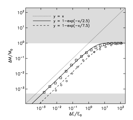
Figure 7: Fractional mass loss defined as the fractional loss of bound stars ($\Delta M/M_{0}$) vs. fractional energy gain ($\Delta E/|E_{0}|$) from the simulations (circles). The dashed line is a simple functional form that makes $\Delta M/M_{0}$ a factor of 7.5 lower than $\Delta E/|E_{0}|$ for $\mbox{$\Delta E/|E_{0}|$}<1$ and flattens to 1 for $\mbox{$\Delta E/|E_{0}|$}>1$. The $\Delta M/M_{0}$ defined as the number of stars beyond $r_{\rm t}$ is shown as squares. A functional fit is shown as a full line. A one-to-one relation is shown as dotted line. The results of the simulations are expected to be between the grey shaded regions, since the maximum value for $\Delta M/M_{0}$ is 1, corresponding to the total disruption of the cluster and the minimum value is 1/8192, when a single star got unbound by the perturbation.

5.2 The cluster disruption time

5.2.1 A toy model for spiral arms in the disc

The strength of a spiral arm perturbation on a cluster depends on $V_{\rm drift}$, $H$ and $\rho_{0}$. In Sections 2.2 and 2.3 and Table 1 we adopted a constant arm-interarm density contrast $\Gamma=10$ and scale length of $H=150\,$pc for gaseous arms, leaving $V_{\rm drift}$ as main $R$ dependent variable.

From equation (2) and $\langle\rho_{\rm HI}\rangle$ from Section 2.2 we find $\rho_{0}=0.33\,\mbox{$M_{\odot}\,{\rm pc}^{-3}$}$. The value of $V_{\rm max}$ in the arm is found from $V_{\rm drift}$ and by considering an acceleration by the arm from $Y_{0}=-2H$ to $Y=0$ (equation 10). With these parameters and Eqs. 13 and 15 we can now calculate the energy gain for clusters that cross spiral arms at different $R$.

With the relation between $\Delta M/M_{0}$ and $\Delta E/|E_{0}|$ from Section 5.1, that is, equation (17) with the factor $f=0.4$, we can estimate the mass loss of the cluster at different $R$. We assume here that $\Delta M/M_{0}$ is independent of $N$, which can be justified since the derivations of $\Delta E/|E_{0}|$ (equations. 8 and 13) are independent of $N$ as well. They do, however, depend on the distribution of stars in the clusters, that is, on the cluster density profile or the concentration index. There might be a small $N$ dependence in the boundary between the impulsive and the adiabatic regime, since clusters with low $N$ are able to adjust faster to a changing potential.

5.2.2 The cluster disruption time

Ostriker et al. (1972) define the cluster disruption time due to many repeated disc shocks ($t_{\rm dd}$) using the impulsive approximation by dividing the initial cluster energy $E_{\rm 0}$ by the energy injection per unit time: $t_{\rm dd}=|\mbox{$E_{\rm 0}$}|/\langle\mbox{${\rm d}$}E/\mbox{${\rm d}$}t\rangle$. For the cluster energy they assume $\mbox{$E_{\rm 0}$}=-0.2\,G\,\mbox{$M_{\rm c}$}/\mbox{$r_{\rm h}$}$ (Note that this implies $\eta=0.4$, see Section 4.1.2). Combined with equation (8) and the fact that clusters have two disc passages per orbital period ($P$), Ostriker et al. (1972) express $t_{\rm dd}$ as

$$t_{\rm dd}=\frac{3\,G\,\mbox{$M_{\rm c}$}\,P\,V^{2}}{20\mbox{$g^{2}_{\rm m}$}\,\mbox{$r^{3}_{\rm h}$}},$$ (18)

This time scale is defined as the time needed to unbind the cluster by (periodically) injecting energy in the cluster by disc shocks. Note that here we have assumed $\mbox{$r^{2}_{\rm h}$}=\mbox{$\bar{r^{2}}$}$. This is true only for very concentrated clusters.

This expression can be rewritten to derive a disruption time due to periodic spiral arm perturbations ($t_{\rm ds}$). We explicitly use the mass loss per spiral arm passage (equation 17), which we approximate as $\mbox{$\Delta M/M_{0}$}=f(\mbox{$\Delta E/|E_{0}|$})$, with $f\simeq 0.4$ (Section 5.1). The expression for $t_{\rm ds}$ can then be derived from

$$\mbox{$t_{\rm ds}$}=\frac{\Delta t}{f}\frac{|\mbox{$E_{\rm 0}$}|}{\Delta E},$$ (19)

with $\Delta E$ from equation (13) (with the adiabatic correction factor) and $\Delta t=\mbox{$t_{\rm drift}$}(R)$. Using the definition of $E_{\rm 0}$ from Section 4.1.2, we can write $\Delta E/|E_{0}|$ as

$$\Delta E/|E_{0}| = \frac{2\mbox{$g^{2}_{\rm m}$}\mbox{$\bar{r^{2}}$}}{3\mbox{$V^{2}_{\rm max}$}}\frac{2\mbox{$r_{\rm h}$}}{\eta G\mbox{$M_{\rm c}$}}\mbox{$A_{\rm w}(x)$}$$ (20)

$$= \frac{4\mbox{$g^{2}_{\rm m}$}}{3\mbox{$V^{2}_{\rm max}$}}\frac{\mbox{$r^{3}_{\rm h}$}}{\eta G\mbox{$M_{\rm c}$}}\frac{\mbox{$\bar{r^{2}}$}}{\mbox{$r^{2}_{\rm h}$}}\mbox{$A_{\rm w}(x)$},$$

where we included a factor $\mbox{$\bar{r^{2}}$}/\mbox{$r^{2}_{\rm h}$}$ to get a dependence on $\mbox{$M_{\rm c}$}/\mbox{$r^{3}_{\rm h}$}$ as in equation (18). For a cluster with $W_{0}=5$ $\mbox{$\bar{r^{2}}$}/\mbox{$r^{2}_{\rm h}$}\simeq 2$.

The adiabatic correction factor ($A_{\rm w}(x)$) of equation (20) is calculated using the results of Section 4. We use the parameters for the $W_{0}=5$ cluster as described in Sections 4.1.3 and 4.2, that is, $\eta=0.41$ and $\bar{\omega}=0.58$. We consider clusters with $\mbox{$M_{\rm c}$}=10^{2}\,\mbox{${\rm M}_{\odot}$},\,10^{3}\,\mbox{${\rm M}_{\odot}$}$ and $10^{4}\,\mbox{${\rm M}_{\odot}$}$ all with $\mbox{$r_{\rm h}$}=3.75\,$pc. The constant radius is based on recent observations of young clusters in spiral galaxies (Larsen, 2004). Using the scaling relations of Section 4.1.2, the values of $\bar{\omega}$ for these clusters are $0.046,0.14$ and $0.46\,$Myr^-1, respectively. In panel A of Fig. 8 we show the result for the impulsive approximation, that is $A(x)=1$, in the top panel and Weinbergs correction factor ($A_{\rm w}(x)$) in the bottom panel.

In panel B of Fig. 8 we show the energy gain of equation (20) using values of $A(x)$ from panel A. For the cluster with $\mbox{$M_{\rm c}$}=10^{2}\,\mbox{${\rm M}_{\odot}$}$ inclusion of the correct $A_{\rm w}(x)$ does not make much difference. For the cluster with $\mbox{$M_{\rm c}$}=10^{3}\,\mbox{${\rm M}_{\odot}$}$, $A_{\rm w}(x)$ decreases to 0.2 at $R_{\rm CR}$ and for the most massive cluster ($\mbox{$M_{\rm c}$}=10^{4}\,\mbox{${\rm M}_{\odot}$}$) the effect of the spiral arm passage is largely damped for almost all values of $R$. This is because $t_{\rm cr}$ is shorter in a more massive cluster, assuming a constant radius.

If we translate $\Delta E/|E_{0}|$ to $\Delta M/M_{0}$ with equation (17) we prevent that the mass loss becomes larger than the cluster mass. Panel C shows $\Delta M/M_{0}$ in the impulsive approximation (top) and with the adiabatic correction factor (bottom). The cluster with $\mbox{$M_{\rm c}$}=10^{2}\,\mbox{${\rm M}_{\odot}$}$ can get completely unbound by a single spiral arm passage ($\Delta M/M_{0}$=1).

An expression for $t_{\rm ds}$ can be obtained by combining Eqs. 19 and 20

$$\mbox{$t_{\rm ds}$}(R)=\frac{3\mbox{$V^{2}_{\rm max}$}}{4g_{\rm m}^{2}}\,\frac{\eta}{f}\frac{1}{\mbox{$A_{\rm w}(x)$}}\frac{G\mbox{$M_{\rm c}$}}{\mbox{$r^{3}_{\rm h}$}}\frac{r_{h}^{2}}{\mbox{$\bar{r^{2}}$}}\,\mbox{$t_{\rm drift}$},$$ (21)

where $\mbox{$V_{\rm max}$}\simeq|\mbox{$V_{\rm drift}$}(R)|$ (equation 1) and $\mbox{$t_{\rm drift}$}=2\pi R/(m|\mbox{$V_{\rm drift}$}|)$, with $m$ the number of spiral arms in the galaxy. In panel D of Fig. 8 we show the result of $t_{\rm ds}$ as a function of $R$ for a two-armed spiral galaxy ($m=2$). For clusters inside the corotation radius, i.e. $R<\mbox{$R_{\rm CR}$}$, the value of $t_{\rm ds}$ is nearly constant. This is because we have assumed the arm parameters not to vary with $R$ (Section 2.2). The variables that are a function of $R$ in equation (21) are $V_{\rm max}$ and $t_{\rm drift}$. The product $V^{2}_{\rm max}\mbox{$t_{\rm drift}$}$ from equation (21) varies with $R$ approximately as $R|1-R/\mbox{$R_{\rm CR}$}|$, since $\mbox{$t_{\rm drift}$}\propto R/|\mbox{$V_{\rm drift}$}|$ and $\mbox{$V_{\rm max}$}\simeq|\mbox{$V_{\rm drift}$}|$ (equation 1). The product $R|1-R/\mbox{$R_{\rm CR}$}|$ increases from 0 at $R=0$ to a maximum at $\mbox{$R_{\rm CR}$}/2$ to decrease again beyond $R=\mbox{$R_{\rm CR}$}/2$. Since at $R_{\rm CR}$ there is never a spiral arm crossing $t_{\rm ds}$ is infinite there.

Figure 8: Evolution of the cluster parameters with $R$ in a two armed grand design spiral galaxy. In the top row results are shown using the impulsive approximation, that is $A(x)=1$, and in the bottom panel we used $A_{\rm w}(x)$ of equation (15). The adiabatic correction factor is shown in panel A. Panel B shows $\Delta E/|E_{0}|$ for a single shock at different $R$. The peak around $R_{\rm CR}$ is because of a minimum in $V_{\rm max}$ around $R_{\rm CR}$. From $\Delta E/|E_{0}|$ we derive $\Delta M/M_{0}$ through equation (17) and the result is shown in panel C. The disruption time at different $R$, $\mbox{$t_{\rm ds}$}(R)$ (equation 21), is shown in panel D. The results for clusters with masses of $10^{2}\,\mbox{${\rm M}_{\odot}$}\,10^{3}\,\mbox{${\rm M}_{\odot}$}$ and $10^{4}\,\mbox{${\rm M}_{\odot}$}$ are shown with dotted, dashed and dotted-dashed lines, respectively. The hashed region indicated the region where $t_{\rm ds}$ is smaller than $t_{\rm drift}$, and therefore $t_{\rm ds}$ from equation (21) can not exist.

6 Discussion and conclusions

Much work has been done on the combined effect of stellar evolution, a realistic stellar mass function and a spherically symmetric Galactic tidal field to understand the dissolution of star clusters. The resulting cluster disruption times of these models (for example Chernoff & Weinberg 1990; Takahashi & Portegies Zwart 2000; Baumgardt & Makino 2003) are longer than the observed values for open clusters in the solar neighbourhood (Lamers et al., 2005) and in the central region of M51 (Gieles et al., 2005). Our study is aimed at understanding the effect of perturbation by spiral arm passages and to see whether they can contribute to this difference.

From the age distribution of open clusters in the solar neighbourhood clusters, Lamers et al. (2005) derived a disruption time of $1.3\times 10^{3}\,$Myr for a $10^{4}\,\mbox{${\rm M}_{\odot}$}$ cluster, which they refer to as $t_{4}$. A similar analysis was performed by Gieles et al. (2005) using the age and mass distribution to derive the disruption time of clusters in the central region of M51. They find $t_{4}\simeq 150\pm 50\,$Myr for clusters with $R<6\,$kpc, that is, within $R_{\rm CR}$ (Section 2). These observed disruption time scales can be compared to the results of Baumgardt & Makino (2003). They derive the disruption time for clusters on a circular motion in the Galaxy and consider a realistic stellar mass function and stellar evolution and the tidal field of the Galaxy. They used a smooth analytical description of the Galaxy potential and find $t_{4}=6.9\times 10^{3}\,$Myr for clusters in the solar neighbourhood, that is, almost a factor of five longer than what is observed. For the parameters of M51, the predicted value of $t_{4}$ is ten times longer than the observed value.

Neither the spiral arm perturbations on a simple cluster, without mass function and stellar evolution (Section 5.2.2), nor the effect of the Galactic tidal field on a realistic cluster can, on their own, explain the observed disruption time. We can compare the disruptive effect of the spiral arm perturbations to the observed values. In Fig. 9 we show the $t_{\rm ds}$ as a function of cluster mass $M_{\rm c}$ for the solar neighbourhood (top panel) and for a grand design spiral galaxy, such as M51 (bottom panel). The parameters of Sections 2 and 5.2.2 are used, that is, the number of spiral arms is four ($m=4$) and $R\simeq 0.9\mbox{$R_{\rm CR}$}$, with $R_{\rm CR}$ the corotation radius, for the solar neighbourhood and $m=2$ and $R\simeq 0.5\mbox{$R_{\rm CR}$}$ for the clusters in M51. The full lines represent the resulting disruption times using the impulsive approximation and the dashed lines show the result for $t_{\rm ds}$ when the correct adiabatic correction is applied. As we showed in Section 5.2.2, the impulsive result applies to clusters with $\mbox{$M_{\rm c}$}\lesssim 3\times 10^{3}\,\mbox{${\rm M}_{\odot}$}$ in the solar neighbourhood, because of the long crossing time $t_{\rm cr}$ of stars in such clusters. For the cluster in a grand design spiral at $R=0.5\mbox{$R_{\rm CR}$}$ the adiabatic correction is important for clusters of slightly higher masses, since at that location $V_{\rm drift}$ is higher (equation 1). In the solar neighbourhood $t_{\rm ds}$ becomes constant for $\mbox{$M_{\rm c}$}\lesssim 10^{2}\,\mbox{${\rm M}_{\odot}$}$. This is because a single arm crossing can destroy clusters with such low masses and $t_{\rm ds}$ becomes equal to $t_{\rm drift}$. The disruption times from the observations of Lamers et al. (2005) and Gieles et al. (2005) for the solar neighbourhood and M51 are indicated as hashed regions in the top and bottom panel, respectively. The area of the hashed region represents the errors in the observations and the mass range of the observed cluster sample. Note that both studies found an empirical mass dependence of $\mbox{$t_{\rm dis}$}\propto\mbox{$M_{\rm c}$}^{0.6}$.

Figure 9: Disruption time due to spiral arm passages ($t_{\rm ds}$) for different $M_{\rm c}$ in the solar neighbourhood (top panel) and in a gra nd design spiral galaxy (bottom). The full lines show the result using the impulsive approximation, that is, equation (21) with $A(x)=1$. The dashed lines show $t_{\rm ds}$ with $A_{\rm w}(x)$ (Fig. 8). The shaded areas are the observed disruption times and mass range of the observed clusters from Lamers et al. (2005) (top) and Gieles et al. (2005) (bottom).

For the solar neighbourhood the disruption time due to the spiral arm perturbations is about an order of magnitude higher than the observed result. For M51 the difference is almost three orders of magnitude. This suggest that spiral arm perturbations contribute little to the disruption of the (low mass) open clusters in the solar neighbourhood and can definitely not explain the observed short disruption time of clusters in M51 (Gieles et al., 2005). In Section 2 we argued that the contribution of the stellar arms, which we have ignored, is even less than that of the gaseous component. This because the time it takes the cluster to cross of stellar arms is much longer than the crossing time of stars in the cluster. This causes the effect of heating by the stellar arms to be largely damped adiabatically (Section 3).

There should thus be a further disruptive agent, which we have not considered so far. The central region of M51 has a rich population of giant molecular clouds (GMCs) (for example Garcia-Burillo et al. 1993) whose velocity with respect to the cluster is relatively small ($\sim 10\,\mbox{km$\,$s${}^{-1}$}$). Even at the relatively large distance from the Galactic centre of the solar neighbourhood there are GMCs with masses $\gtrsim 10^{6}\,\mbox{${\rm M}_{\odot}$}$ (for example Solomon et al. 1987).

References

- Athanassoula (1984) Athanassoula E., 1984, Phys. Rep., 114, 321
- Athanassoula (1992) Athanassoula E., 1992, MNRAS, 259, 345
- Bastian et al. (2005) Bastian N., Gieles M., Lamers H. J. G. L. M., Scheepmaker R. A., de Grijs R., 2005, A&A, 431, 905
- Baumgardt & Makino (2003) Baumgardt H., Makino J., 2003, MNRAS, 340, 227
- Binney & Tremaine (1987) Binney J., Tremaine S., 1987, Galactic dynamics. Princeton, NJ, Princeton University Press, 1987
- Bissantz et al. (2003) Bissantz N., Englmaier P., Gerhard O., 2003, MNRAS, 340, 949
- Cayatte et al. (1994) Cayatte V., Kotanyi C., Balkowski C., van Gorkom J. H., 1994, AJ, 107, 1003
- Chernoff & Weinberg (1990) Chernoff D. F., Weinberg M. D., 1990, ApJ, 351, 121
- de Grijs & van der Kruit (1996) de Grijs R., van der Kruit P. C., 1996, A&AS, 117, 19
- Dehnen (2000) Dehnen W., 2000, AJ, 119, 800
- Dehnen (2002) Dehnen W., 2002, in Athanassoula E., Bosma A., Mujica R., eds, ASP Conf. Ser. 275: Disks of Galaxies: Kinematics, Dynamics and Peturbations Our Galaxy. pp 105–116
- Drimmel (2000) Drimmel R., 2000, A&A, 358, L13
- Drimmel & Spergel (2001) Drimmel R., Spergel D. N., 2001, ApJ, 556, 181
- Egusa et al. (2004) Egusa F., Sofue Y., Nakanishi H., 2004, PASJ, 56, L45
- Fux (2001) Fux R., 2001, A&A, 373, 511
- Garcia-Burillo et al. (1993) Garcia-Burillo S., Guelin M., Cernicharo J., 1993, A&A, 274, 123
- Georgelin & Georgelin (1976) Georgelin Y. M., Georgelin Y. P., 1976, A&A, 49, 57
- Gieles et al. (2005) Gieles M., Bastian N., Lamers H. J. G. L. M., Mout J. N., 2005, A&A, 441, 949
- Gieles et al. (2006) Gieles M., Portegies Zwart S. F., Baumgardt H., Athanassoula E., Lamers H. J. G. L. M., Sipior M., Leenaarts J., 2006, MNRAS, 371, 793
- Gnedin et al. (1999) Gnedin O. Y., Lee H. M., Ostriker J. P., 1999, ApJ, 522, 935
- Gnedin & Ostriker (1997) Gnedin O. Y., Ostriker J. P., 1997, ApJ, 474, 223
- Gnedin & Ostriker (1999) Gnedin O. Y., Ostriker J. P., 1999, ApJ, 513, 626
- Gonzalez & Graham (1996) Gonzalez R. A., Graham J. R., 1996, ApJ, 460, 651
- Harris (1996) Harris W. E., 1996, VizieR Online Data Catalog, 7195, 0
- Heggie & Mathieu (1986) Heggie D. C., Mathieu R. D., 1986, LNP Vol. 267: The Use of Supercomputers in Stellar Dynamics, 267, 233
- Holtzman et al. (1992) Holtzman J. A., Faber S. M., Shaya E. J., Lauer T. R., Groth J., Hunter D. A., Baum W. A., Ewald S. P., et al. 1992, AJ, 103, 691
- Kharchenko et al. (2005) Kharchenko N. V., Piskunov A. E., Röser S., Schilbach E., Scholz R.-D., 2005, A&A, 438, 1163
- King (1962) King I., 1962, AJ, 67, 471
- King (1966) King I. R., 1966, AJ, 71, 64
- Kranz et al. (2001) Kranz T., Slyz A., Rix H.-W., 2001, ApJ, 562, 164
- Kundic & Ostriker (1995) Kundic T., Ostriker J. P., 1995, ApJ, 438, 702
- Lamers et al. (2005) Lamers H. J. G. L. M., Gieles M., Bastian N., Baumgardt H., Kharchenko N. V., Portegies Zwart S., 2005, A&A, 441, 117
- Lamers et al. (2005) Lamers H. J. G. L. M., Gieles M., Portegies Zwart S. F., 2005, A&A, 429, 173
- Larsen (2004) Larsen S. S., 2004, A&A, 416, 537
- Larsen et al. (2001) Larsen S. S., Brodie J. P., Elmegreen B. G., Efremov Y. N., Hodge P. W., Richtler T., 2001, ApJ, 556, 801
- Levine et al. (2006) Levine E. S., Blitz L., Heiles C., 2006, Science, 312, 1773
- Makino et al. (2003) Makino J., Fukushige T., Koga M., Namura K., 2003, PASJ, 55, 1163
- Martos et al. (2004) Martos M., Hernandez X., Yáñez M., Moreno E., Pichardo B., 2004, MNRAS, 350, L47
- McMillan & Hut (1996) McMillan S. L. W., Hut P., 1996, ApJ, 467, 348
- Murali & Weinberg (1997) Murali C., Weinberg M. D., 1997, MNRAS, 291, 717
- Nakai et al. (1994) Nakai N., Kuno N., Handa T., Sofue Y., 1994, PASJ, 46, 527
- Nieten et al. (2006) Nieten C., Neininger N., Guélin M., Ungerechts H., Lucas R., Berkhuijsen E. M., Beck R., Wielebinski R., 2006, A&A, 453, 459
- Oort (1958) Oort J. H., 1958, Ricerche Astronomiche, 5, 507
- Ostriker et al. (1972) Ostriker J. P., Spitzer L. J., Chevalier R. A., 1972, ApJ, 176, L51+
- Portegies Zwart et al. (2001) Portegies Zwart S., McMillan S. L. W., Hut P., Makino J., 2001, MNRAS, 321, 199
- Rix & Rieke (1993) Rix H.-W., Rieke M. J., 1993, ApJ, 418, 123
- Roberts (1969) Roberts W. W., 1969, ApJ, 158, 123
- Rots et al. (1990) Rots A. H., Bosma A., van der Hulst J. M., Athanassoula E., Crane P. C., 1990, AJ, 100, 387
- Schweizer (1976) Schweizer F., 1976, ApJS, 31, 313
- Seigar & James (1998) Seigar M. S., James P. A., 1998, MNRAS, 299, 685
- Solomon et al. (1987) Solomon P. M., Rivolo A. R., Barrett J., Yahil A., 1987, ApJ, 319, 730
- Spitzer (1987) Spitzer L., 1987, Dynamical evolution of globular clusters. Princeton, NJ, Princeton University Press, 1987, 191 p.
- Spitzer (1958) Spitzer L. J., 1958, ApJ, 127, 17
- Spitzer & Chevalier (1973) Spitzer L. J., Chevalier R. A., 1973, ApJ, 183, 565
- Sygnet et al. (1988) Sygnet J. F., Tagger M., Athanassoula E., Pellat R., 1988, MNRAS, 232, 733
- Tagger et al. (1987) Tagger M., Sygnet J. F., Athanassoula E., Pellat R., 1987, ApJ, 318, L43
- Takahashi & Portegies Zwart (2000) Takahashi K., Portegies Zwart S. F., 2000, ApJ, 535, 759
- van der Kruit (1988) van der Kruit P. C., 1988, A&A, 192, 117
- van der Kruit & Searle (1981a) van der Kruit P. C., Searle L., 1981a, A&A, 95, 105
- van der Kruit & Searle (1981b) van der Kruit P. C., Searle L., 1981b, A&A, 95, 116
- van der Kruit & Searle (1982a) van der Kruit P. C., Searle L., 1982a, A&A, 110, 61
- van der Kruit & Searle (1982b) van der Kruit P. C., Searle L., 1982b, A&A, 110, 79
- Weinberg (1994a) Weinberg M. D., 1994a, AJ, 108, 1398
- Weinberg (1994b) Weinberg M. D., 1994b, AJ, 108, 1403
- Weinberg (1994c) Weinberg M. D., 1994c, AJ, 108, 1414
- Whitmore et al. (1999) Whitmore B. C., Zhang Q., Leitherer C., Fall S. M., Schweizer F., Miller B. W., 1999, AJ, 118, 1551
- Wielen (1971) Wielen R., 1971, A&A, 13, 309
- Zimmer et al. (2004) Zimmer P., Rand R. J., McGraw J. T., 2004, ApJ, 607, 285
- Zwicky (1955) Zwicky F., 1955, PASP, 67, 232