The use of neural networks to probe the structure of the nearby universe

Abstract

In the framework of the European VO-Tech project, we are implementing new machine learning methods specifically tailored to match the needs of astronomical data mining. In this paper, we shortly present the methods and discuss an application to the Sloan Digital Sky Survey public data set. In particular, we discuss some preliminary results on the 3-D taxonomy of the nearby ($z<0.5$) universe. Using neural networks trained on the available spectroscopic base of knowledge we derived distance estimates for $\sim 30$ million galaxies distributed over $\sim 8,000$ sq. deg. We also use unsupervised clustering tools to investigate whether it is possible to characterize in broad morphological bins the nature of each object and produce a reliable list of candidate AGNs and QSOs.

1 Introduction

Modern photometric digital surveys performed with dedicated instruments are in fact producing high quality multiband data at a huge rate, and a new generation of software tools is being developed to merge databases and to extract patterns, trends, etc. Furthermore, due the ongoing efforts to build a Virtual Observatory (VO) infrastructure (cf. the European VO-Tech, [1]), everyone will have at his fingertips the possibility to extract and manipulate such multi-wavelength, multi-epoch, multi-instrument datasets of huge dimensionality. The extraction of useful information from such datasets imposes to abandon old conceptual schemes largely based on the 3-D visualization capability of human minds, and to introduce in the astronomical practice fine tuned, machine learning methods for statistical pattern recognition, classification and visualization [2]. In this context, however, astronomical data pose non trivial problems due to the fact that they are usually highly degenerate, present strong non linear correlations among parameters and are plagued by large fraction of missing data and upper limits.

In what follows we shall shortly outline the first results of our ongoing effort to implement and apply a new generation of tools to the construction of a 3-D taxonomy of the nearby universe with a characterization of galaxy types in a few, broadly defined, catagories: normal (early and late type) galaxies, AGN, QSO, etc.

For all the experiments described below, we used the Sloan Digital Sky Survey Data Release 4 and/or 5 (hereafter SDSS4/5; [3]) which provides photometric data in 5 bands for several hundred million galaxies distributed over $\sim 8,000$ square degrees, together with additional spectroscopic information for a subsample (hereafter SpS) of $\sim 10^{6}$ galaxies. Such spectroscopic information include, among other things, redshifts and a spectral classification index derived from an eigenvector analysis which allows to disentangle among normal galaxies (SP2), stars (SP1), nearby AGN (SP3), distant AGN (SP4), late type stars (SP6). This spectroscopic base of knowledge can be used as a training ground for interpolative and supervised methods as well as a validation ground for unsupervised ones.

2 The photometric redshift

One of the main sources of degeneracy in the photometric properties of galaxies is the lack of information on their distances and therefore any attempt to partition the parameter space requires first the derivation of distance estimates. In order to evaluate photometric redshifts we made use of an improved version [4] of the Neural Networks (NNs) method presented in [5]. Both steps are accomplished using NNs architecture known as MLP (Multi Layer Perceptron).

We adopted a two steps approach based on the use of MLP [6, 7]. First we trained a MLP to recognize nearby (id est with redshift $z<0.25$) and distant ($z>0.25$) objects, then we trained two separate MLPs to work in the two different redshift regimes. Such approach finds support in the fact that in the SDSS-5 catalogue, the distribution of galaxies inside the two different redshift intervals is dominated by two different galaxy populations: the Main Galaxy (MG) sample in the nearby region, and the Luminous Red Galaxies (LRG) in the distant one. The use of two separate networks ensures that the NNs achieve a good generalization capabilities in the nearby sample, leaving the biases mainly in the distant one.

To perform the separation between MG and LRG objects, we extracted from the SDSS-4 SpS training, validation and test sets weighting, respectively, $60\%$, $20\%$ and $20\%$ of the total number of objects (449,370 galaxies). The resulting test set, therefore, consisted of 89,874 randomly extracted objects.

After the first network has classified the objects in nearby and distant ones, the derivation of the photometric redshifts is performed separately in the two regimes. Since NNs are excellent at interpolating data but very poor in extrapolating them, in order to minimize the systematic errors at the extremes of the training redshift ranges we adopted the following procedure. For the nearby sample we trained the network using objects with spectroscopic redshift in the range $\left[0.0,0.27\right]$ and then considered the results to be reliable in the range $\left[0.01,0.25\right]$. In the distant sample, instead, we trained the network over the range $\left[0.23,0.50\right]$ and then considered the results to be reliable in the range $\left[0.25,0.48\right]$.

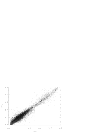
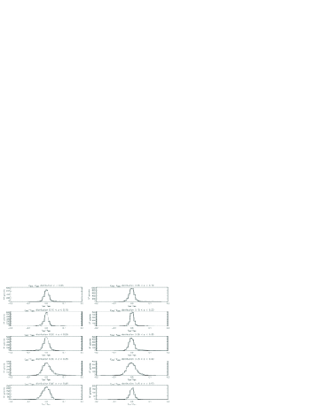
Figure 1: Left: distribution of spectroscopic versus photometric redshifts in the test set. Lighter grey points mark LRG galaxies. Notice the larger scatter of non-LRGs in the distant ($z>0.25$) sample. Right: distribution of the errors computed over redshift bins for the distant sample.

The error for our redshift estimates has been evaluated on the test set by measuring the dispersion of points in the $z_{spec}$ vs $z_{phot}$ plane, i. e. the variance of the $z_{spec}-z_{phot}$ variable, after performing an interpolative correction in order to correct for systematics. The results can be summarized as follows:

• For the MG sample, in the best experiment, the robust variance turned out to be $\sigma_{3}=0.0208$ over the whole redshift range and $0.0197$ and $0.0245$ for the nearby and distant objects, respectively.

• For LRG sample we obtained $\sigma_{3}\simeq 0.0163$ over the whole range, and $\sigma_{3}\simeq 0.0154$ and $\sigma_{3}\simeq 0.0189$ for the nearby and distant samples, respectively.

3 The clustering

The implementation of a reliable classification scheme based on photometric information only, is an old problem in astronomy [8]. In few words, it consists in partitioning the observed parameter space in clusters of objects sharing some underlying common physical property. Obviously, since there is no a priori reason to assume that photometric classification must reflect strictly any morphological classification (actually the degeneracy observed in colours strongly argues against it), any effective classification method must be unsupervised, id est it must partition the photometric parameter space using only the statistical properties of the data themselves. We therefore implemented a hierarchical approach which starts from a preliminary clustering performed using as unsupervised clustering algorithm the so called ”Probabilistic Principal Surfaces” or PPS, and then makes use of the Negative Entropy concept and of a dendrogram structure to agglomerate the clusters found in the first phase.

3.1 PPS - Principal Probabilistic Surfaces

Probabilistic Principal Surfaces (PPS) [9, 10] are a nonlinear extension of principal components, in that each node on the PPS is the average of all data points that projects near/onto it. PPS define a non-linear, parametric mapping ${\mathbf{y}}({\mathbf{x}};{\mathbf{W}})$ from a $Q$-dimensional latent space $({\mathbf{x}}\in{\mathbf{R}}^{Q})$ to a $D$-dimensional data space $({\mathbf{t}}\in{\mathbf{R}}^{D})$, where normally $Q<<D$. The function ${\mathbf{y}}({\mathbf{x}};{\mathbf{W}})$ (defined continuous and differentiable) maps every point in the latent space to a point into the data space.

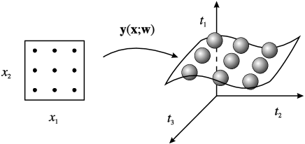
Figure 2: Scheme of a latent variable model mapping a $3$D data space onto a $2$D latent space with latent variables uniformly arranged. Each latent variable is mapped, through the nonlinear function $y$, to the center of a Gaussian distribution.

Since the latent space is $Q$-dimensional, these points will be confined to a $Q$-dimensional manifold non-linearly embedded into the $D$-dimensional data space. In our method, the points belonging to the parameter space will be projected on the surface of a 2-dimensional sphere. The visualization capabilities of the PPS can prove very useful in several aspects of the data interpretation phase such as, for instance, the localization of data points lying far away from the more dense areas (outlayers), or of those lying in the overlapping regions between clusters, or to identify data points for which a specific latent variable is responsible. A visualization of the data clustering is achieved by PPS algorithm through the projection of objects from the multi-parametric $D$-dimesional space to a two dimensional surface. These clusters, representing groups of objects corresponding to the same latent variable, are then decimated using NEC: a hyerarchical non supervised agglomeration algorithm.

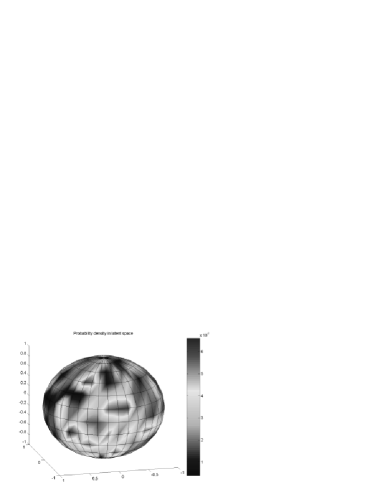
Figure 3: Probability density function of the SDSS data plotted on the latent sphere surface.

3.2 NEC - Negentropy Clustering

Most unsupervised methods require the number of clusters to be provided a priori. This circumstance represents a serious problem when exploring large and complex data sets where the number of clusters can be very high or, in any case, unpredictable. A simple treshold criterium is not satisfactory in most astronomical applications due to the high degeneracy and the noisiness of the data which lead to the erroneous agglomeration of data.

We introduce the Fisher’s linear discriminant which is a classification method that first projects high-dimensional data onto a line, and then performs a classification in the projected one-dimensional space [6]. The projection is performed in order to maximize the distance between the means of the two classes while minimizing the variance within each class. On the other hand, we define the differential entropy H of a random vector ${\mathbf{y}}=(y_{1},\ldots,y_{n})^{T}$ with density $f({\mathbf{y}})$ as $H({\mathbf{y}})=\int f({\mathbf{y}})\log f({\mathbf{y}})d{\mathbf{y}}$ so that negentropy $J$ can be defined as $J(\mathbf{y})=J({\mathbf{y}}_{Gauss})-H(\mathbf{y})$, where $\mathbf{y}_{Gauss}$ is a Gaussian random vector of the same covariance matrix as $\mathbf{y}$. Negentropy can be interpreted as a measure of non-Gaussianity and, since it is invariant for invertible linear transformations, it is obvious that finding an invertible transformation that minimizes the mutual information is roughly equivalent to finding directions in which the Negentropy is maximized.

Our implementation of the method makes use of an approximation to Negentropy which provides a good compromise between the properties of the two classic non-Gaussianity measures given by kurtosis and skeweness. Negentropy can be used to agglomerate the clusters (regions) found by the PPS and the only a priori information is a dissimilarity threshold $T$. Let us suppose to have $c$ multi-dimensional regions $X_{i}$ with $i=1,\ldots,c$ that have been defined by the PPS. The NEC algorithm, in practice, measures whether two clusters can or cannot be modeled by one single Gaussian or, in other words, if the two regions can be considered to be just aligned or rather as a part of a larger data set. By increasing the value of the dissimilarity treshold, the number of clusters decreases and robust partitions produce plateaus in the ”treshold vs number of clusters” diagram

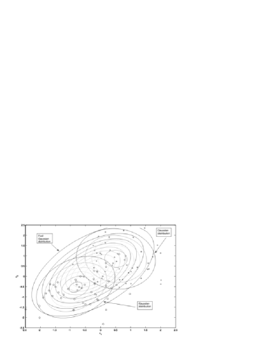
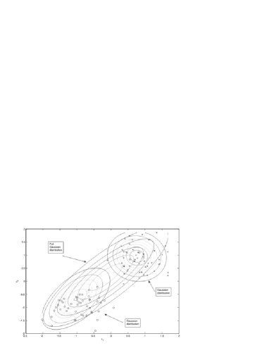
Figure 4: Exemplification of how the NEC algorithm works on two Gaussian distribution examples. Left: Negentropy = $2.6261$ using the $G_{1}$ function with $a_{1}=0.1$; Right: Negentropy = $0.005$ using the $G_{1}$ function with $a_{1}=0.1$

3.3 Preliminary results on clustering

We first applied the PPS algorithm to the sample of spectroscopically selected SDSS DR-4 objects using as parameters for the clustering the 4 colours obtained from model magnitudes (u-g,g-r,r-i,i-z) of SDSS archive. We fixed the number of latent variables and latent bases of the PPS to 614 and 51 respectively, so obtaining at the end of this step 614 clusters, each formed by objects which only respond to a certain latent variables. We choose a large number of latent variables in order to obtain an accurate separation of objects and to avoid that any group of distinct but near points in the parameter space could be projected onto the same cluster by chance. The clusters found by the PPS are graphically represented by groups of points with the same colour (a different colour for each cluster) on the surface of a 2-d sphere embedded in the 3-dimensional latent space. These first order clusters were then fed to the NEC algorithm which determined the final number of clusters. The plateau analysis of the agglomerative process and the inspection of the dendrogram allowed to set the treshold to a value corresponding to 31 clusters. We present in table (1) the ten most populous clusters together with the distribution of the specClass index within each cluster. The additional 21 clusters represent less than 10 $\%$ of the objects and are still under investigation. It needs to be emphasized that the clustering makes use of the photometric data only and the spectroscopic information is used only to validate them. As it can be seen, galaxies (SP2) clearly dominate clusters 1, 2 and 6. Whether this separation reflects or not some deeper differences among the three groups (such as, for instance, different morphologies), cannot be assessed on the grounds of presently available data. AGNs (SP3) dominate clusters 5 and 9 even though some contamination from galaxies exists.

Cl. n	SP0	SP1	SP2	SP3	SP4	SP6
1	69	145	9362	48	0	12
2	25	133	13370	10	0	12
3	149	132	63	64	0	5
4	44	3396	1530	189	67	1
5	202	85	447	2428	6	10
6	26	125	13728	12	0	12
7	0	0	0	0	0	484
8	1	1	1	0	0	329
9	541	1507	127	4750	18	1
10	89	474	2117	19	4	529

Table 1: The table shows the distribution of objects in the most significant clusters found by our procedure. The columns correspond to different values of the specClass index.

Late type stars (SP6) populate mainly clusters 7 and 8 and are strong contaminants of cluster 10 which also is dominated by galaxies.

4 Conclusions

We have produced a catalogue of redshifts for all galaxies in the SDSS database matching the following selection criteria and falling in the redshift range $0.005-0.5$. These redshifts have been used to produce a first 3-D map of the nearby universe which is currently under study to identify structures and to define accurate selection functions. Much work has instead still to be done in obtaining a reliable partition in hogeneous types. This is partly due to the lack of a reliable data sets for labeling and partly to a still poor understanding of how to deal in an effective way with upper limits and missing data.

Acknowledgements: this work was sponsored by the Italian MIUR through a PRIN grant and by the European Union through the VO-Tech project. The authors wish to thank G. Miele, G. Raiconi and N. Walton for useful discussions.

References

- [1] WWW site: http://eurovotech.org.
- [2] Staiano A., De Vico L., Ciaramella A., Donalek C., Longo G., Raiconi G., Tagliaferri R., Amato R., Del Mondo C., Mangano G. & Miele G., 2005, IEEE, in print.
- [3] Adelman-McCarthy J., et al., 2007, ApJS, submitted.
- [4] D’Abrusco R., Staiano A., Longo G., Brescia M., De Filippis E., Paolillo & Tagliaferri R. 2006, ApJ, submitted.
- [5] Tagliaferri R., Longo G., Andreon S., Capozziello S., Donalek C., & Giordano ,G., 2003, Lectures Notes in Computer Science, 2859, 226.
- [6] Bishop C. M., 1995, Neural Networks for Pattern Recognition, Oxford University Press.
- [7] Duda R.O., Hart P.E., Stork D.G., 2001, Pattern Classification, John Wiley & Sons Inc., Second Edition.
- [8] de Vaucouleurs G, de Vaucouleurs A., Corwin H.C. jr, 1976, Second Reference Catalogue of Bright Galaxies, University of Texas Press.
- [9] Chang K., 2000, Nonlinear Dimensionality Reduction Using Probabilistic Principal Surfaces, PhD Thesis, The University of Texas at Austin (USA).
- [10] Staiano A. 2003, Unsupervised Neural Networks for the Extraction of Scientific Information from Astronomical Data, PhD thesis, University of Salerno (Italy).