Optical multi-band observations of BL Lacertae during the outburst of 2005
Abstract
The aim of our observations is to investigate the intranight variability properties and the spectral variability of BL Lacertae. 799 optical multi-band observations were intensively made with the Beijing-Arizona-Taiwan-Connecticut (BATC) 60/90cm Schmidt telescope during the outburst composed of two subsequent flares in 2005. The second flare, whose rising phase lasted at least 44 days, was observed with amplitudes of more than 1.1 mag in three BATC optical bands. In general, on intranight timescale the amplitude of variability and the variation rate are larger at the shorter wavelength, and the variation rate is comparable in the rising and decaying phases within each band. A possible time lag between the light curves in bands e and m, around 11.6 minutes, was obtained. Based on the analysis of the colour index variation with the source brightness, the variability of BL Lacertae can be interpreted as having two components: a “strongly-chromatic” intranight component and a “mildly-chromatic” internight component, which may be the results of both intrinsic physical mechanism and geometric effects.
keywords:
galaxies: BL Lacertae objects: general – BL Lacertae objects: individual: BL Lacertae – galaxies: photometry1 Introduction
BL Lacertae (BL Lac) is the prototype of BL Lac objects(BL Lacs). In the unified scheme of radio-loud active galactic nuclei (AGNs), BL Lacs and flat-spectrum radio quasars (FSRQs) are usually collectively termed as blazars. BL Lacs are characterized by non-thermal continuum emission across the whole electromagnetic spectrum with absent or weak emission and absorption lines (e.g. Stickel, Fried & Kühr 1993, ), variable and high polarization (e.g. Angel & Stockman 1980, ; Impey & Neugebaur 1988, ; Gabuzda et al. 1989, ), large amplitude and rapid variability at all wavelengths from radio to -rays (e.g. Ravasio et al. 2002, ; Böttcher et al. 2003, ) and superluminal motion of radio components (e.g. Denn, Mutel & Marscher 2000). BL Lac is a well-studied source that has been monitored in optical band for more than a century. Variability on both long and short timescales has been observed by many authors (Villata et al. 2004a, , and references therein). Microvariability has been detected since the early work by Racine racine (1970). Intranight optical variability (INOV) of this object was studied in detail during the long 1997 outburst. Nesci et al. nesci (1998) reported multi-band INOV based on the observations made in July 1997. The source was never found to be stable during their campaign. They found that the amplitude of flux variation was always larger at shorter wavelengths and no apparent time lags among the light curves in different wavebands could be detected. Speziali & Natali speziali (1998) monitored BL Lac in three optical bands on three nights in August 1997. Their results involved INOV on timescale ranging from 30 minutes up to 3.5 hours. They concluded that the magnitude of variability was larger at shorter wavelengths and the source showed a marked trend to become bluer when brighter. This chromatism of INOV was confirmed by many other authors (e.g. Matsumoto et al. 1999, ; Ghosh et al. 2000, ; Clements & Carini 2001, ). Papadakis et al papadakis (2003) analyzed the INOV, the timescales of rising and decaying processes, and the time lags between different optical bands. Their results showed that the variability amplitudes increased with increasing frequency. The rising and decaying timescales were comparable within each band, but increased with decreasing frequency. The time lag between the light curves in bands B and I was less than 0.4 hours. They also detected significant spectral variations, which had the trend to become harder (bluer) as the flux increased.
In order to investigate the details of the physical processes and geometric conditions based on the brightness and spectral variability, BL Lac has been intensively monitored in four campaigns (see Ravasio et al. 2002, ; Villata et al. 2002, ; Böttcher et al. 2003, ; Villata et al. 2004a, ; Villata et al. 2004b, ) by the Whole Earth Blazar Telescope (WEBT) collaboration since 1999 to 2003. Most of these optical multi-band data were collected and analyzed by Villata et al. 2004a . Their results from the analysis of colour index revealed that the variability had two components, long term (a few-day timescale) “mildly-chromatic” variations and strong bluer-when-brighter chromatic short term variations (intraday flares). Stalin et al. stalin (2006) showed that BL Lac became bluer when brighter on intranight timescale, while this trend was less significant on internight timescale. Their results may also suggest that the variability of BL Lac has two components. They found that the dependence of the spectral variability on its brightness was different from that of S5 0716+714. On the contrary, some objects were reported to become redder when brighter. For example, Ramirez et al ramirez (2004) presented that the spectrum of PKS 0736+017 became redder when brighter on both internight and intranight timescales. This different property may be introduced by different physical processes or physical environments.
To shed more light on the INOV and spectral variation with respect to flux variation on both internight and intranight timescales, we carried out dense observations on BL Lac. We describe the observations and data reduction in the following section. Sect. 3 gives the results of our observations. A summary is presented in Sect. 4.
2 Observations and data reduction
Our observations were carried out with a 60/90cm f/3 Schmidt telescope, which is located at the Xinglong Station of the National Astronomical Observatories of China. The telescope is equipped with a 15-colour intermediate-band photometric system, covering a wavelength range of 3 000–10 000 Å. A Ford Aerospace CCD camera is mounted at its main focus. The CCD has a pixel size of 15 microns and its field of view is , resulting in a resolution of 1.7″/pixel. The telescope and the photometric system are mainly used to carry out the BATC survey (Zhou 2005, ).
We performed optical observations in the BATC e, i and m bands in a cyclic mode. Their central wavelengths are 4885, 6685 and 8013 Å, respectively. For good compromise between photometric precision and temporal resolution, the exposure times were 150 seconds in the BATC i band and mostly 240 seconds in the e and m bands. Because a frame size of pixels () is large enough to cover BL Lac and its comparison stars, we only read out the central pixels of the CCD images. The readout time is about 5.6 seconds. So we can achieve a temporal resolution of about 12 minutes in each band. This quasi-simultaneous measurements enable us to investigate the colour variation. BL Lac was observed on 26 nights during the period from July 5, 2005 to November 18, 2005.
All images were processed with the automatic data reduction procedure including bias subtraction, flat fielding, position calibration, aperture photometry and flux calibration. The adopted aperture radius was 4 pixels (6.8″), since the average FWHM of the object and the comparison stars was 3.5″. The inner and outer radii of the sky annulus were set as 6 and 9 pixels (10.2″and 15.3″), respectively. The comparison stars B, C and H from Smith et al. smith (1985) were used for flux calibration. Their BATC magnitudes were obtained by observing them and three BATC standard stars, HD 19445, HD 84937 and BD+17d4708, on a photometric night. They were listed in Table 1. The star ID is followed by its BATC e, i, m magnitudes and errors in Table 1. The BATC magnitudes of BL Lac can be obtained by differential photometry. The BATC magnitudes can also be transferred to standard Johnson-Cousins magnitudes by the relations obtained by Zhou et al. zhou2003 (2003). The details on data reduction procedure were described by Yan et al. yan (2000) and Zhou et al. zhou2003 (2003). Our photometry results are listed in Tables 2–4. These three tables have the same format. The universal date of observations (Col. 1) is followed by the universal time at the middle of exposure (Col. 2), Julian date at the middle of exposure (Col. 3), exposure time (Col. 4), BATC magnitudes (Col. 5), photometry error (Col. 6) and the difference, (it is the difference between the differential magnitude of comparision stars B, C , and the average of . x indicates the BATC band e, i or m.), which indicates the confidence of the observations (Col. 7). These three full tables are only available in electronic form.
| star | e | i | m |
|---|---|---|---|
| ID | (mag) | (mag) | (mag) |
| B | 13.8930.011 | 12.1480.010 | 11.5920.005 |
| C | 14.8590.018 | 13.9700.012 | 13.7550.012 |
| H | 15.2290.025 | 13.9130.013 | 13.5090.010 |
| UT Date | UT | JD | Exposure Time | e | ||
|---|---|---|---|---|---|---|
| yyyy/mm/dd | hh:mm:ss | (day) | (seconds) | (mag) | (mag) | (mag) |
| 2005/07/05 | 19:05:25 | 2453557.29541 | 240 | 16.126 | 0.032 | -0.003 |
| 2005/07/05 | 19:19:26 | 2453557.30518 | 240 | 16.079 | 0.032 | 0.003 |
| 2005/07/06 | 19:20:50 | 2453558.30615 | 300 | 16.239 | 0.050 | 0.000 |
| 2005/07/15 | 17:59:35 | 2453567.24976 | 240 | 16.011 | 0.078 | 0.029 |
| 2005/07/15 | 18:16:18 | 2453567.26123 | 240 | 16.008 | 0.064 | 0.036 |
| UT Date | UT | JD | Exposure Time | i | ||
|---|---|---|---|---|---|---|
| yyyy/mm/dd | hh:mm:ss | (day) | (seconds) | (mag) | (mag) | (mag) |
| 2005/07/05 | 19:09:31 | 2453557.29834 | 150 | 14.840 | 0.012 | -0.011 |
| 2005/07/05 | 19:24:42 | 2453557.30884 | 150 | 14.866 | 0.012 | 0.011 |
| 2005/07/06 | 19:28:01 | 2453558.31104 | 180 | 14.982 | 0.016 | 0.000 |
| 2005/07/15 | 18:05:46 | 2453567.25391 | 150 | 14.762 | 0.018 | 0.014 |
| 2005/07/15 | 18:20:33 | 2453567.26416 | 150 | 14.818 | 0.018 | 0.024 |
| UT Date | UT | JD | Exposure Time | m | ||
|---|---|---|---|---|---|---|
| yyyy/mm/dd | hh:mm:ss | (day) | (seconds) | (mag) | (mag) | (mag) |
| 2005/07/05 | 19:13:40 | 2453557.30127 | 240 | 14.258 | 0.013 | 0.003 |
| 2005/07/05 | 19:28:46 | 2453557.31152 | 240 | 14.245 | 0.014 | -0.003 |
| 2005/07/06 | 19:33:59 | 2453558.31519 | 300 | 14.410 | 0.018 | 0.000 |
| 2005/07/15 | 18:10:36 | 2453567.25732 | 240 | 14.205 | 0.017 | -0.005 |
| 2005/07/15 | 18:24:56 | 2453567.26733 | 240 | 14.205 | 0.017 | -0.010 |
3 Results
3.1 Light curves
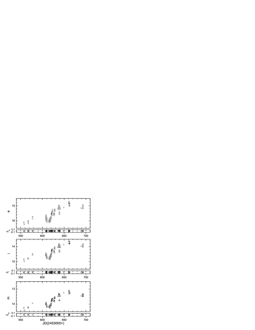
The light curves in bands e, i and m are displayed in Fig. 1. Our photometry clearly shows that BL Lac is violent and varies from day to day during the period of our more than four months (JD from 2453557 to 2453693) monitoring. One can see two flares apparently from Fig. 1. The rising phase of the second flare lasted 44 days (JD 2453617–2453661). The amplitudes of variation during the second flare are 1.374, 1.252 and 1.174 mag in bands e, i and m, respectively. The variability amplitudes increased with increasing frequency. It is a pity that we did not completely record these two flares due to the weather conditions or other campaigns.
One can see that many fast oscillations superimposed on the long term variations. Our multi-band observations on many nights gave us the opportunity to intensively investigate the intranight variability. The criterion presented by Jang & Miller jang (1997) was adopted to decide whether the source was variable or not. It is defined as , where is the standard deviation of the source magnitude, are the standard deviation of . Because presents the variation of the comparison stars, indicates the observational error that provides a more accurate determination of the actual error than the normal photometric error. is taken as the confidence level of variability. The source will be claimed to be variable at 99% confidence level when . The object is decided to be variable only when at least in two bands if it is monitored in three or more bands (Jang & Miller jang, 1997; Stalin et al. stalin, 2006). To quantitatively analyze the INOV, the intranight variability amplitude is defined as (Heidt & Wagner 1996, ):
| (1) |
where , and are the average, maximum and minimum of the magnitudes on one light curve. is the same as what is described above.
There are 19 out of 26 nights on which the data points are more than 5 in each band. The confidence level of variability was calculated for these 19 nights in each band. According to the criterion described above, the object was variable on 9 nights. The intranight variability amplitude, , was calculated for these 9 “variable nights”. The variability amplitude in band e is generally larger than those in bands i and m. The average values are 1.22%, 1.00% and 0.82%, respectively. It is larger at the higher frequency. This is consistent with the results of Nesci et al. nesci (1998), Speziali & Natali speziali (1998) and Papadakis et al. papadakis (2003). In order to compare the variation rates of the light curves in different bands at both the rising and decaying phases, we fitted the light curves on the 9 “variable nights” with a linear model. The slope of the linear least square fitting is taken as the variation rate. Fig. 2 gives examples of linear fittings on four nights. One can see from Fig. 2 that the light curves in three bands are consistent with each other. All the analysis results are listed in Table 5, in which the universal date of observations (Col. 1) is followed by the number of frames in each band (Col. 2), the confidence level of variability with the label of being variable or not (Col. 3, V/N indicates the source is variable or not.), the intranight variability amplitude (Col. 4), the variation rates and their errors in the rising and decaying parts (Col. 5 and Col. 6). The statistic results show that the variation rates of the light curves in band e is larger than those in bands i and m both in the rising and decaying parts. It is larger in the shorter wavebands in general. The average values of the variation rate are 0.065, 0.057 and 0.042 in the e, i and m bands for the rising parts, respectively, while for the decaying phases, they are respectively 0.064, 0.061 and 0.051. The variation rates are comparable in the rising and decaying phases.
| Date | Band | C(V/N) | Y | ||
|---|---|---|---|---|---|
| mm/dd | (N) | % | |||
| 07/15 | e(7) | 2.217(N) | |||
| i(7) | 1.264(N) | ||||
| m(7) | 1.845(N) | ||||
| 08/25 | e(14) | 4.385(V) | 2.09 | 7.74.3 | |
| i(14) | 1.909(N) | 1.15 | 6.30.7 | ||
| m(14) | 4.489(V) | 0.93 | 3.40.6 | ||
| 08/26 | e(9) | 4.262(V) | |||
| i(9) | 1.221(N) | ||||
| m(9) | 1.446(N) | ||||
| 08/27 | e(8) | 3.538(V) | |||
| i(8) | 0.918(N) | ||||
| m(7) | 1.276(N) | ||||
| 09/02 | e(6) | 2.853(V) | 0.88 | 7.23.9 | |
| i(6) | 3.187(V) | 0.39 | 5.21.5 | ||
| m(6) | 2.655(V) | 0.51 | 5.81.2 | ||
| 09/03 | e(12) | 1.785(N) | |||
| i(12) | 0.934(N) | ||||
| m(12) | 1.136(N) | ||||
| 09/05 | e(16) | 3.349(V) | 1.12 | 3.51.0 | |
| i(16) | 1.779(N) | 1.07 | 4.00.3 | ||
| m(16) | 4.008(V) | 0.91 | 3.00.3 | ||
| 09/06 | e(11) | 1.325(N) | |||
| i(11) | 1.556(N) | ||||
| m(11) | 1.831(N) | ||||
| 09/07 | e(20) | 1.687(N) | |||
| i(20) | 1.440(N) | ||||
| m(20) | 2.859(V) | ||||
| 09/08 | e(24) | 3.343(V) | 1.21 | 10.22.0 | 0.6 |
| i(24) | 2.285(N) | 1.19 | 9.20.7 | 0.2 | |
| m(24) | 4.105(V) | 0.87 | 6.90.7 | 0.3 | |
| 09/09 | e(9) | 3.929(V) | |||
| i(13) | 1.760(N) | ||||
| m(13) | 1.016(N) | ||||
| 09/13 | e(14) | 5.487(V) | 0.76 | 1.2 | |
| i(14) | 5.605(V) | 0.85 | 0.6 | ||
| m(14) | 5.069(V) | 0.67 | 0.7 | ||
| 09/14 | e(13) | 2.712(V) | 1.00 | 5.91.2 | |
| i(13) | 2.874(V) | 0.87 | 5.80.4 | ||
| m(13) | 3.047(V) | 0.73 | 3.60.5 | ||
| 09/24 | e(17) | 2.349(N) | |||
| i(17) | 1.450(N) | ||||
| m(17) | 2.063(N) | ||||
| 09/25 | e(8) | 2.338(N) | |||
| i(8) | 1.029(N) | ||||
| m(8) | 1.474(N) | ||||
| 09/26 | e(8) | 1.964(N) | 0.88 | 3.52.7 | |
| i(8) | 5.477(V) | 1.15 | 6.20.6 | ||
| m(8) | 2.800(V) | 0.53 | 2.90.7 | ||
| 10/17 | e(10) | 1.384(N) | |||
| i(10) | 1.332(N) | ||||
| m(10) | 1.624(N) | ||||
| 10/18 | e(24) | 3.306(V) | 1.41 | 2.80.4 | |
| i(24) | 3.932(V) | 0.83 | 1.80.1 | ||
| m(24) | 2.992(V) | 0.93 | 1.90.1 | ||
| 11/18 | e(17) | 4.507(V) | 1.59 | 11.21.8 | 3.8 |
| i(17) | 3.481(V) | 1.47 | 7.10.4 | 1.3 | |
| m(17) | 5.289(V) | 1.28 | 6.30.5 | 1.0 |

3.2 Time lag
It can be noticed that the shape of the light curves in three bands are very similar (see Figs. 1 and 2). To look for correlations and possible time lags between them, the z-transform discrete correlation function (ZDCF, Alexander alexander, 1997) was applied to the light curves on “variable nights” that were determined to have INOV. ZDCF is an improvement of the discrete correlation function (DCF). ZDCF applies z transformation to the correlation coefficients and uses equal population bins rather than the equal time bins in DCF (Edelson & Krolik 1988, ). The calculation of ZDCF requires that the light curves must have at least 12 points (Alexander alexander, 1997). The ZDCFs between the light curves in band e and m are illustrated in Fig. 3. The ZDCFs in three nights without enough observation points are not good. So we only use the good ZDCFs in three nights to obtain the result. The time lag was calculated by three methods. is the time lag corresponding to the maximum of ZDCF, and are the time lags calculated as centroid (see Raiteri et al. 2003, ; Raiteri et al. 2005, ) and by Gaussian fit, respectively. They are listed in Table 6. The columns of Tabel 6 are the date of observation, the maximum of ZDCF and the time lags by three methods followed by their errors. The time lags reveal that the variations in band e lead the variations in band m. The average of the time lags by three methods is 0.194 hours (11.6 minutes). It is in excellent agreement with the lag obtained by Papadakis et al. papadakis (2003) on Jul. 5, 2001, 0.23 hours between band B and I. These two results are all larger than 3 minutes obtained by Stalin et al. stalin (2006) between band V and R on Oct. 22, 2001. But the different separation of band frequency must be considered. An upper limit to the possible time delay (10 minutes) between band B and I of 0716+714 obtained by Villata et al. villata2000 (2000) suggests that our result is reasonable. It should be treated with caution, since it is close to the temporal resolution of observation in each band.

| Date | Max | |||
|---|---|---|---|---|
| mm/dd | (hour) | (hour) | (hour) | |
| 09/08 | 0.724 | 0.236 | 0.2760.082 | |
| 10/18 | 0.736 | 0.156 | 0.2250.337 | |
| 11/18 | 0.770 | 0.147 | 0.1070.095 |
3.3 Spectral variability
The relationship between the optical spectral variability and the brightness variation was investigated by many authors for a number of BL Lacs (see e.g. Speziali & Natali speziali, 1998; Papadakis et al. papadakis, 2003; Raiteri et al. 2003, ; Villata et al. 2004a, ; Wu et al. 2005, ; Stalin et al. stalin, 2006). D’Amicis et al. (damicis, 2002) reported that the spectra of all their 8 BL Lac samples became bluer when they got brighter. Similar results were obtained by Fiorucci et al. fiorucci (2004). However Ramirez et al (ramirez, 2004) showed that the spectrum of a FSRQ PKS 0736+017 became red with increased brightness. Gu et al. (gu, 2006) found that all their 5 BL Lacs tended to be bluer as they turned brighter, while two out of three FSRQs tended to be redder when they were brighter. Villata et al. (villata2006, 2006) reported that FSRQs 3C 454.3 generally had the redder-when-brighter behaviour during the 2004-2005 outburst. The variation rate between the colour index (or spectral index) and the brightness of each source studied above was different.

Based on our high temporal resolution observations, the spectral variability with the brightness was investigated in this section. The colour index , which was calculated by coupling the BATC e and m magnitudes taken within 20 minutes, was adopted to denote the optical spectral slope. We took to denote the brightness of the source. In our analysis, the contribution of the host galaxy was not subtracted from the total flux densities. But the results are not strongly affected by the host galaxy, since it has colours similar to the AGN. Figs. 4. a–c display the relationship between colour index and brightness on three “variable nights”. Only the most densely observed three nights were plotted as examples, similar results can be obtained from the data on other “variable nights”. Solid lines are the best fittings to the data points. b is the fitted slope followed by its error. Fig. 4. d gave the relationship between the obtained 258 colour indices and their brightness during our monitoring. One can obviously see that the values of for intranight points were larger than that in Fig. 4. d. It suggests that the spectral variability of the intranight fast flares and internight variability may be different. To decompose the intranight variation from the internight variation, we used the faintest magnitudes in bands e and m on each observation night to indicate the internight long term variation. Then the intranight variations were obtained by subtracting the magnitudes from the maximum for each night. The relationships between the colour index and the brightness were drawn in Figs. 4. e and f for the internight variations and the intranight fast flares, respectively. The linear correlations are all significant at a 0.95 confidence level, while the slope of fast flares () is larger than that of internight variations (). So the spectral variability reveals that the variability has “strongly chromatic” intranight fast flares and “mildly chromatic” internight variations. Our result is consistent with that of Villata et al. 2004a . The slopes in this work are larger than the slopes by Villata et al. (2004a, ), since the considered frequency separation in this work is larger than that in Villata et al. (2004a, ).
4 Summary
We monitored BL Lac with a high temporal resolution with BATC telescope during the period from July 5, 2005 to November 18, 2005. Many fast variations superposed on the long term trend were recorded. The rising phase of the second flare lasted at least 44 days. During this rising process, the variability amplitudes are 1.374, 1.252 and 1.174 mag in band e, i and m, respectively. 799 optical multi-band observations and 258 colour indices were obtained. By analyzing the INOV, we conclude that for the intranight variability, the amplitude of variability is larger at the shorter wavelength, the variation rate is also larger at shorter wavelength and it is comparable in the rising and decaying phases within each band. An average time lag between bands e and m was obtained by the method of ZDCF. It must be treated with caution, because it is close to the temporal resolution of our observations. Different variation rates in different bands and the time lag will lead to spectrum variations. The variability of BL Lac can be interpreted as having two components by the analysis of spectral variability with the brightness: a “strongly-chromatic” intranight component and a “mildly-chromatic” internight component. Our results confirmed the conclusions about the components of the variability from Villata et al. (2004a, ).
In the generally accepted scenario, the non-thermal emission from BL Lacs includes low frequency synchrotron radiation and high frequency inverse-Compton radiation, which are produced by relativistic electrons in a jet oriented at a small angle to the line of sight. The jet is powered and accelerated by a supermassive black hole surrounded by an accretion disk (e.g. Ghisellini et al. 1998, ). Although the details are still under debate, this scenario can well explain most of the observation properties of BL Lacs (see e.g. Böttcher & Bloom 2000, ). The combination of “strongly-chromatic” intranight variability and “mildly-chromatic” internight variability is possible induced by both intrinsic mechanisms and geometrical effects. The “mildly-chromatic” component can be interpreted by the variation of Doppler factor on a spectrum slightly deviating from a power law (Villata et al. 2004a, ). The direction of the jet varies as the knots move relativistically on helical trajectories within an small angle with respect to the observer. The internight variations can be introduced by the variation of the direction of jet adding the spectrum slightly deviating from the power law. The “strongly-chromatic” component can be explained by particle acceleration and propagation by shock-in-jet events (e.g. Mastichiadis & Kirk 2002, ). The particles are accelerated by the shocks advancing down the jet, the optical synchrotron emission is enhanced due to the accelerated particles and the over-dense magnetic field. This kind of shock-in-jet model will lead to a bluer-when-brighter phenomenon (Marscher & Travis 1996, ), which is the same as the spectral variability in this paper. The intranight component can also be explained by a simple model representing the variability of a synchrotron component (Vagnetti, Trevese & Nesci 2003, ). So the variability of BL Lac may be the results of both intrinsic mechanisms and geometric effects.
Acknowledgments
We owe great thanks to all the BATC staffs who make great efforts to this campaign. We are grateful to the referee for valuable comments and detailed suggestions that have been adopted to improve this paper very much. This research is supported by the National Natural Science Foundation of China under Grants 10433010 and 10521001. This work is partly supported by the Youth Growth Foundation of Shandong University at Weihai.
References
- (1) Alexander T., 1997, in Maoz D., Sternberg A., Leibowitz E. M., eds, Astronomical Time Series. Dordrecht, Kluwer, p. 163
- (2) Angel J. R. P., Stockman H. S., 1980, ARA&A, 18, 321
- (3) Böttcher M., Bloom S. D., 2000, AJ, 119, 469
- (4) Böttcher M. et al., 2003, ApJ, 596, 847
- (5) Clements S. D., Carini M. T., 2001, AJ, 121, 90
- (6) D’Amicis R., Nesci R., Massaro E., Maesano M., Montagni F., D’Alessio F., 2002, PASA, 19, 111
- (7) Denn G. R., Mutel L. R., Marscher A. P., 2000, ApJS, 129,61
- (8) Edelson R. A., Krolik J. H., 1988, ApJ, 333,646
- (9) Fiorucci M., Ciprini S., Tosti G., 2004, A&A, 419, 25
- (10) Gabuzda D. C., Cawthorne T. V., Roberts D. H., Wardle J. F. C., 1989, ApJ, 347, 701
- (11) Ghisellini G., Celotti A., Fossati G., Maraschi L., Comastri A., 1998, MNRAS, 301, 451
- (12) Ghosh K. K., Ramsey B. D., Sadun A. C., Soundararajaperumal S., Wang J., 2000, ApJ, 537, 638
- (13) Gu M. F., Lee C.-U., Pak S., Yim H. S., Fletcher A. B., 2006, A&A, 450, 39
- (14) Heidt J., Wagner S. J., 1996, A&A, 305, 42
- (15) Impey C. D., Neugebaur G., 1988, AJ, 95, 307
- (16) Jang M., Miller H. R., 1997, AJ, 114, 565
- (17) Marscher A. P., Travis J. P., 1996, A&AS, 120, 537
- (18) Mastichiadis A., Kirk J. G., 2002, PASA, 19, 138
- (19) Matsumoto K., Kato T., Nogami D., Kawaguchi T., Kinnunen T., Poyner G., 1999, PASJ, 51, 253
- (20) Nesci R., Maesano M., Massaro E., Montagni F., Tosti G., Fiorucci M., 1998, A&A, 332, L1
- (21) Papadakis I. E., Boumis P., Samaritakis V., Papamastorakis J., 2003, A&A, 397, 565
- (22) Racine R., 1970, ApJ, 159, 99L
- (23) Raiteri C. M. et al., 2003, A&A, 402, 151
- (24) Raiteri C. M. et al., 2005, A&A, 438, 39
- (25) Ramirez A., de Diego J. A., Dultzin-Hacyan D., Gonzalez-Perez J. N., 2004, A&A, 421, 83
- (26) Ravasio M. et al., 2002, A&A, 383, 763
- (27) Smith P. S., Balonek T. J., Heckert P. A., Elston R., Schmidt G. D., 1985, AJ, 90, 1184
- (28) Speziali R., Natali G., 1998, A&A, 339, 382
- (29) Stalin C. S., Gopal-Krishna G.-K., Sagar Ram, Wiita Paul J., Mohan V., Pandey A. K., 2006, MNRAS, 366, 1337
- (30) Stickel M., Fried J. W., Kühr H., 1993, A&AS, 98, 393
- (31) Vagnetti F., Trevese D., Nesci R., 2003, ApJ, 590, 123
- (32) Villata M. et al., 2000, A&A, 363, 108
- (33) Villata M. et al., 2002, A&A, 390, 407
- (34) Villata M. et al., 2004a, A&A, 421, 103
- (35) Villata M. et al., 2004b, A&A, 424, 497
- (36) Villata M. et al., 2006, A&A, 453, 817
- (37) Wu J. H., Peng B., Zhou X., Ma J., Jiang Z. J., Chen J. S., 2005, AJ, 129, 1818
- (38) Yan H. J. et al., 2000, PASP, 112, 691
- (39) Zhou X. et al., 2003, A&A, 397, 361
- (40) Zhou X., 2005, JKAS, 38, 203