A Particle Simulation for the Global Pulsar Magnetosphere: the Pulsar Wind linked to the Outer Gaps

Abstract

Soon after the discovery of radio pulsars in 1967, the pulsars are identified as strongly magnetic (typically $10^{12}$G) rapidly rotating ($\sim 10^{2}-0.1$ Hz) neutron stars. However, the mechanism of particle acceleration in the pulsar magnetosphere has been a longstanding problem. The central problem is why the rotation power manifests itself in both gamma-ray beams and a highly relativistic wind of electron-positron plasmas, which excites surrounding nebulae observed in X-ray. Here we show with a three dimensional particle simulation for the global axisymmetric magnetosphere that a steady outflow of electron-positron pairs is formed with associated pair sources, which are the gamma-ray emitting regions within the light cylinder. The magnetic field is assumed to be dipole, and to be consistent, pair creation rate is taken to be small, so that the model might be applicable to old pulsars such as Geminga. The pair sources are charge-deficient regions around the null surface, and we identify them as the outer gap. The wind mechanism is the electromagnetic induction which brings about fast azimuthal motion and eventually trans-field drift by radiation drag in close vicinity of the light cylinder and beyond. The wind causes loss of particles from the system. This maintains charge deficiency in the outer gap and pair creation. The model is thus in a steady state, balancing loss and supply of particles. Our simulation implies how the wind coexists with the gamma-ray emitting regions in the pulsar magnetosphere.

1 Introduction

Our particle simulation follows the historic gedanken experiments by Goldreich & Julian (1969) and by Jackson (1976), in which a rotating neutron star with aligned magnetic moment is put in vacuum, and motion of charged particles around the star are explored. Electromagnetic induction by the star produces a quadrupolar electric field in the surrounding space with a surface charge on the star. The electric force is so large that the surface charge is pulled out into the magnetosphere. For the fate of these charged particles, it was shown by the earlier simulations (Krause-Polstorff & Michel 1985a; 1985b, hereafter KM) that the magnetosphere settles down into a quiet state with electronic domes above the polar caps, a positronic or ionic equatorial disc and vacuum gaps in the middle latitudes. (For definite of sign of charge, we consider a parallel rotator rather than an anti-parallel rotator; with this polarity the polar caps are negatively charged and the equatorial region is positively charged.) The quiet solution has no energy release at all. However, the gaps are unstable against pair creation cascade, which is the subject of our simulation for an active magnetosphere.

Before describing the results of our simulation, let us consider how plasma density and dissipation processes affect the magnetic filed structure. Here, we restrict ourselves to the axisymmetric case for which many works have been done. In the limit of low density, the electromagnetic fields around the star is vacuum ones, and the magnetic field lines are closed. As has been shown by the previous particle simulation (KM), for a moderate density of plasmas, the electromotive force by the star manifests itself in strong charge separation. The magnetosphere contains the gaps in between the polar domes and the equatorial disc. It is known that convective current by the corotating clouds with finite extent is not enough to open the magnetic field (KM, Kaburaki 1982, Fitzpatrick & Mestel 1988).

To obtain the quiet solutions with finite extent of plasmas in space, the total charge of the system $Q$ is assumed to be non-zero. If $Q=0$, the corotating plasma will extend to the light cylinder and possibly beyond the light cylinder (KM). However, such a solution has yet to be discussed seriously. Rylov (1978) and Fitzpatrick & Mestel (1988) considered a flow beyond the light cylinder in closed magnetic filed lines. In this case, non-electromagnetic force such as radiation drag and inertial force is required for a self-consistent steady solution. The reaction force due to rotational bremsstrahlung may be important: the radiation reaction force becomes comparable to the Lorentz force when $\gamma\sim(3BR_{c}^{2}/2q)^{1/4}\equiv\gamma_{r}$, where $B$ is the magnetic field strength, $R_{c}$ is the curvature radius, and $q$ is the charge of a particle. A typical value of $\gamma_{r}$ is $\sim 3\times 10^{7}(\mu_{30}/P)^{1/4}$ for electrons, where $P$ is the rotation period in seconds and $\mu_{30}$ is the magnetic moment in $10^{30}{\rm G}\;{\rm cm}^{3}$. The value of $\gamma_{r}$ is still smaller in a region where the magnetic field is weaken in vicinity of the equatorial neutral sheets. The expected global flow pattern is circular, being similar to the electric quadrupolar fields, starting from the star, going beyond the light cylinder and returning back to the star. A possibility is also pointed out that both positive and negative particles may leave the star to make a wind toward infinity in the steady state (Jackson 1976, Fitzpatrick, & Mestel 1988).

Contrary to the case of moderate densities, the force-free model assumes high density neutral plasmas and imposes the boundary conditions that the magnetic field is opened. However, the appropriate boundary condition for the force-free problem is still controversial (Uzdensky 2003). It has been shown that the separatrix, which is the open-close boundary, should not have a sheet current if the Y-point is located on the light cylinder, and that a wedge-shaped electric-field-dominant region ($E>B$) appears beyond the light cylinder (Uzdensky 2003). Ogura and Kojima (2003) obtains a numerical solution of the force-free magnetosphere, and find that electric field becomes larger than the magnetic field in a region beyond a few light-cylinder radii, suggesting break down of the force-free approximation. Relativistic magnetohydrodynamic simulation also requires some dissipation in vicinity of the magnetic neutral sheet, where magnetic field lines are closed (Komissarov 2006). Thus, the force-free model suggests that most part of the magnetic flux will be open, but some flux might be closed with dissipation in the equatorial neutral sheet.

In any case, the force-free approximation requires sources of copious quasi-neutral plasmas. Young pulsars such as Crab will have a high rate of pair creation, and therefore the open filed structure may be plausible in a large part of the magnetosphere. On the other hand, for older pulsars such as Geminga, the pair creation rate is lower, and therefore a larger gap and closed field structure may be plausible. Our study starts with a simulation for the latter low-density case in which the magnetic filed is assumed to be dipole. To be consistent, pair creation rate is assumed to be low. Cases with higher densities shall be treated in subsequent papers. Our result will be helpful also for understanding the electrodynamics in the dissipative domain with closed magnetic fields.

2 Method of Simulation

In the first step of our calculation, we have reproduced the quiet solution. However, it must be noted here that we use a distinctively different method. In the previous works, to reduce load in calculation, the particles are assumed to follow magnetic field lines and to obey the Aristotelian mechanics, i.e., the particles are put at rest if the exerting force vanishes. We solve the relativistic equation of motion for each particle like particle-in-cell (PIC) methods, so that we treat gyro-motion and any kinds of drift motions. The mass-charge ratio of the simulation super-particles is taken to be so small that gyro-motion is kept always microscopic. In the case of actual pulsars, gyro-motion can be macroscopic if the Lorentz factor $\gamma$ is increased up to the maximum reachable value $\gamma_{\rm max}$, which corresponds to the available voltage of the star, in other words, the potential drop across the polar caps. However, this would not be the case because not all the available voltage is used for field-aligned acceleration in the gaps, and radiation drag prevents $\gamma$ from increasing. In our simulation, typical gyro-radii for the light cylinder magnetic field are $\sim 5\times 10^{-4}\gamma R$, where $\gamma$ is the Lorentz factor of the super-particles, and $R$ is the stellar radius. The value of $\gamma_{\rm max}$ for the super-particles is 2000. In the simulation, $\gamma\ll\gamma_{\rm max}$, so that gyro-radii are always much smaller than $R$. As mentioned before, we take the radiation drag force into account in our equation of motion, which becomes

$${d\mbox{\boldmath$p$}_{i}\over dt}=q_{i}(\mbox{\boldmath$E$}+\mbox{\boldmath$\beta$}_{i}\times\mbox{\boldmath$B$})+\mbox{\boldmath$F$}_{r},$$ (1)

where $\mbox{\boldmath$\beta$}_{i}$ is the velocity of the $i$-th particle in units of the light speed; $\mbox{\boldmath$p$}_{i}=m\gamma_{i}\mbox{\boldmath$\beta$}_{i}$, $\gamma_{i}=(1-\mbox{\boldmath$\beta$}_{i}\cdot\mbox{\boldmath$\beta$}_{i})^{-1/2}$; $m$ and $q_{i}$ ($=+q$ or $-q$) is the mass and charge of the particles; $\mbox{\boldmath$F$}_{r}=(2/3)(q_{i}^{2}/R_{c}^{2})\gamma_{i}^{4}(\mbox{\boldmath$p$}_{i}/|\mbox{\boldmath$p$}_{i}|)$ represents the radiation drag force.

Unlike typical PIC, the electric field is calculated in use of a Green’s function with the boundary condition that the stellar surface is a perfect conductor. The method enables us to keep exactly the corotational potential on the stellar surface. We calculate the electric field and particle motion in three dimension, and therefore the scheme itself is fully three dimensional. The model we considered is axisymmetric because of the boundary condition of aligned rotator. The electric field is composed of the vacuum part $\mbox{\boldmath$E$}_{v}$, which is produced by a rotating star in vacuum, and the particle part $\mbox{\boldmath$E$}_{m}$, which is produced by particles in the magnetosphere:

$$\mbox{\boldmath$E$}(\mbox{\boldmath$r$})=\mbox{\boldmath$E$}_{v}(\mbox{\boldmath$r$})+\mbox{\boldmath$E$}_{m}(\mbox{\boldmath$r$})=-\nabla\phi_{v}-\nabla\phi_{m}$$ (2)

with

$$\phi_{v}=\left\{\begin{array}[]{lr}\displaystyle{B_{s}R\;\Omega\over 6}\left[3\left(r\over R\right)^{2}\sin^{2}\theta-2\right],&(r\lid R)\\ \displaystyle B_{s}R\left[-{\Omega\over 6}\left(R\over r\right)^{3}(3\cos^{2}\theta-1)+Q{R\over r}\right],&(r>R)\end{array}\right.$$ (3)

and

$$\phi_{m}=\sum^{n}_{i=1}q_{i}\left[{1\over|\mbox{\boldmath$r$}-\mbox{\boldmath$r$}_{i}|}-{R/r_{i}\over|\mbox{\boldmath$r$}-(R/r_{i})^{2}\mbox{\boldmath$r$}_{i}|}-{1-R/r_{i}\over|\mbox{\boldmath$r$}|}\right],$$ (4)

which yields

$$\mbox{\boldmath$E$}_{m}(\mbox{\boldmath$r$})=\sum_{i=1}^{n}q_{i}\left[{\mbox{\boldmath$r$}-\mbox{\boldmath$r$}_{i}\over|\mbox{\boldmath$r$}-\mbox{\boldmath$r$}_{i}|^{3}}-\frac{R}{r_{i}}{\mbox{\boldmath$r$}-(R/r_{i})^{2}\mbox{\boldmath$r$}_{i}\over|\mbox{\boldmath$r$}-(R/r_{i})^{2}\mbox{\boldmath$r$}_{i}|^{3}}-\frac{(1-R/r_{i})\mbox{\boldmath$r$}}{r^{3}}\right],$$ (5)

where $r$ is the position vector for a given point, $q_{i}$ and $\mbox{\boldmath$r$}_{i}$ are the charge and the position of the $i$-th particle, and $n$ is the particle number; $B_{s}$ is the magnetic field strength at the poles, $\Omega=R/R_{L}$ is the non-dimensional angular velocity, and $Q$ is the non-dimensional net-charge in units of $B_{s}R^{2}$. Freedom of the net-charge of the system $Q$ is included in $\mbox{\boldmath$E$}_{v}$. The Green’s function, the brackets in (4), is composed of Coulomb potentials by the particles in the magnetosphere and their mirror charges, so that $\phi_{m}$ satisfies the boundary conditions, $\phi_{m}=$ constant on the stellar surface and $\phi_{m}\rightarrow 0$ at infinity. Since $\mbox{\boldmath$E$}_{v}$ represents the corotation electric field by the star, $\mbox{\boldmath$E$}_{v}+\mbox{\boldmath$E$}_{m}$, is automatically guaranteed to be the corotational electric field on the stellar surface. In general, surface charge appears, and field-aligned electric force exerts on it. We, therefore, replace the surface charge by simulation particles in each step of time, so that the surface charge can move into the magnetosphere freely.

In (4), we neglect the retardation effect. By this neglect, the calculation of the electric field becomes simply summing-up of Coulomb forces, which can be done very quickly by the special purpose computer for astronomical $N$-body problem, GRAPE (Sugimoto et al. 1990; Makino et al. 1997). Typical use of GRAPE is for stellar dynamics. Note that GRAPE has sign-bits and applies to the Coulomb forces. Omission of retardation is not serious as far as an axisymmetric and steady state is concerned, while introduction of GRAPE makes us possible to perform this heavy calculation.

For realistic simulation of the active pulsars, we take into account electron-positron pair creation. If there is a very large electric field along the magnetic field, particles are accelerated to emit curvature gamma-rays which converted into pairs by interaction with soft photons from the stellar surface or with strong magnetic field near the star. In our simulation, we omit detailed pair creation processes and assume that pairs are created if a region has a field-aligned electric field larger than a critical value $E_{cr}$. For the results presented in this paper, $E_{cr}=0.25B_{L}$, where $B_{L}$ is the light cylinder magnetic field. The creation rate is a simulation parameter and limited by ability of computer. In the present calculation, typically $1600$ particles are created per rotation. The total number of particles is $\sim 5\times 10^{4}$ in a steady state.

As prescribed by our choice of the Green’s function, the boundary condition for the electric potential has already been included, i.e., the corotational potential (or $E_{\theta}=B_{s}\Omega\sin\theta\cos\theta$) on the stellar surface and $\phi\rightarrow 0$ at infinity. It is a distances of about $10R_{L}$ that the electric potential vanishes within the accuracy of the calculation, which is $1.5\times 10^{-2}B_{L}R_{L}$ in our simulation. While the outer boundary condition for the electric filed is given at infinity, we put an outer boundary for particles at $R_{out}=10R_{L}$, so that the particles flowing out across the outer boundary are removed, and no particles come into the simulation domain across it, and thereby we save the number of particles. We also used $R_{out}=20R_{L}$, and $30R_{L}$ to check the effect of the outer boundary. For the initial condition, we started with a vacuum magnetosphere, and suppress pair creation until the static solution by KM is reached. Once we establish the static solution, then pair creation is switched on. The simulation parameters are $\Omega=R/R_{L}=0.2$, $m/q=10^{-5}$, and $B_{L}=(1/2)\Omega^{3}B_{s}=4\times 10^{-3}B_{s}$.

3 Results and Discussion

After several rotation-periods of time, the magnetosphere settles into a steady state with electronic polar outflows and positronic equatorial outflows, which are mixed in the middle latitudes (see the top panels of Fig. 1). Some particles are circulating in the magnetosphere. However, the rest of the particles forms the wind. A region around the null surface produces electron-positron pairs steadily, and the accelerating electric field is kept slightly larger than $E_{\rm cr}$, typically $\sim 1.5E_{\rm cr}$. In the course to the steady state, after the onset of pair creation, the gaps diminish both in size and in electric field strength: the original gap field is screened out down to $E_{cr}$, except for the geometrically small gaps locating around the null surface at axial distances of $\sim 0.5R_{L}$ ( the bottom panels of Fig. 1b). This region is identified as the outer gap (Cheng, Ho & Ruderman 1986; Takata, Shibata & Hirotani 2004) which has been proposed to explain the gamma-ray beams. The bottom right panel of Fig. 1 shows that the field-aligned electric field is unscreened in the gaps. On the other hand, the outside of the gaps as well as inside the polar domes and the equatorial disc, the plasmas screen out the field-aligned electric field.

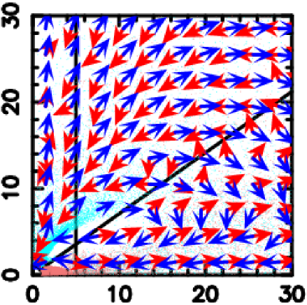
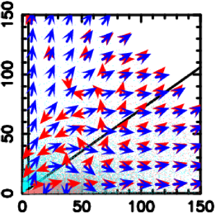
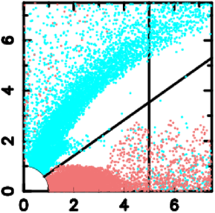
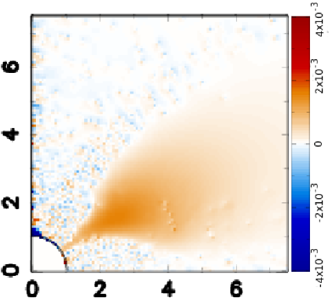
Figure 1: Top left panel: The velocity fields (arrows) and the positions of the particles (dots) on the meridional plane. The red arrows and light red dots are for positive particles, and the blue arrows and light blue dots are for negative particles. The geometrical scale length is normalized by the stellar radius, and the light-cylinder corresponds to the axial distance of 5. The inclined line in the middle latitude indicates the null surface for the dipole field, on which the Goldreich-Julian charge density vanishes. Top right panel: The same, but for the outer magnetosphere. Bottom left panel: The outer gap appears at axial distance of $\sim 3$ around the null surface, where the positive particles are ejected to the right, and the negative particles to the left. Only the particle positions are shown. Bottom right panel: The strength of the field-aligned electric fields.

The positrons ejected from the outer gap accumulate in the equatorial disc which grows in size with time. Due to strong induction of rotation, the azimuthal velocity of the disc plasma increases with distance toward the speed of light, and the Lorentz factor is found to increase until radiation reaction becomes important. Since the radiation drag is in azimuthal direction, the drift across the closed magnetic field causes the radial outflow of the positrons (Fig. 1). Interestingly the global electric field becomes such that the equatorial disc super-corotates as shown in Fig. 2, and as a result, radiation drag becomes efficient before the very vicinity of the light-cylinder, $\sim 0.8R_{L}$. Because the azimuthal motion is due to $E_{\perp}$ cross $B$ drift, the perpendicular electric field $E_{\perp}$ plays an essential role for the wind mechanism. Of the positrons drifting across the field, about one half flows out of the system, while the other half drifts to higher latitudes and turns back to the star.

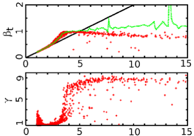
Figure 2: The azimuthal velocity of the particles in the disc ($|z|\leq 0.2$) (upper panel) and the corresponding Lorentz factor (lower panel) as functions of the axial distance in units of the stellar radius. The light radius is located at the axial distance of $\varpi=5$, and the Lorentz factor is found to increase around $\varpi\sim 4$. The dashed green curve indicates the $E_{\perp}$-drift velocity, $E_{\perp}/B$, calculated formally from the local fields. The saturation Lorentz factor by the drag is $\gamma_{r}\sim 14$ for the super particle (corresponding to $\gamma_{r}=10^{4}-10^{5}$ for real electrons) and is 4% of $\gamma_{\rm max}$

On the other hand, electrons produced in the outer gap are absorbed by the star. However, the equivalent amount is re-emitted from the polar caps at higher latitudes. As a result, the electron domes grow and expand across the light cylinder. In the steady state, the property of the polar domes changes spatially from the corotating parts near the star to the sub-rotating parts in higher altitudes as shown in Fig. 3, where the azimuthal velocity is indicated by colors with the electric iso-potentials. The boundaries of the colors are vertical in the corotating parts, while they bend in the sub-rotating parts, in which field-aligned motion becomes appreciable. In the electron clouds extending further out with axial distances of $\sim 1.5R_{L}$, increase of the azimuthal velocity ($E_{\perp}$-acceleration) causes increase of the Lorentz factor and the drag force. About one half of the polar electrons flows out of the system nearly along the magnetic field lines (the centrifugal outflow), while the other half drifts across the field lines significantly due to radiation drag, and turns back to the star.

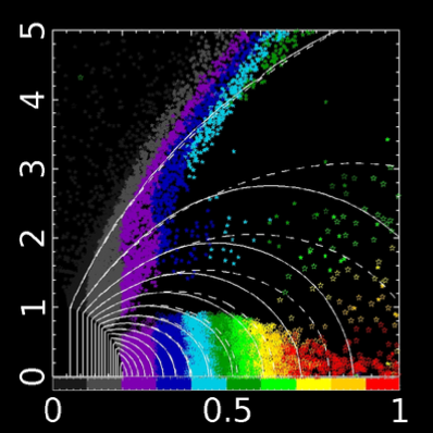
Figure 3: The azimuthal velocity (color coded) of the particles (dots) and the contours of the electric potential (dashed-curves) with the fields lines (solid curves). The meaning of the colors is shown in the color bar just below the equatorial plane, where each color indicates the corotation speed at each axial distance.

Concerning the electric property of the magnetosphere, we find it most remarkable that the net charge $Q$ of the system (the star plus magnetosphere) almost vanishes. In the previous works (KM; Smith, Michel & Thacker 2001), a positive $Q$, e.g. our initial value $Q=1/3$ (equivalent to $+10$ of KM with their choice of the unit charge), is assumed to obtain a finite extent of the plasma clouds, and it was suggested that if $Q\sim 0$, the clouds may expand to the light cylinder. We have started with a positive $Q=1/3$. It is notable that our simulation includes creation and loss of particles, and the dynamics determines the stable value of $Q$. In the final steady state, the positive $Q$ disappears. More precisely, $Q$ is kept slightly negative so as for electrons to be pushed and escape. The net charge $Q$ is adjusted so that the same amounts of the negative and positive particles flow out steadily.

To see that the particles which are removed at the outer boundary really leave from the star, we made a convergency study with $R_{out}=10R_{L}$, $20R_{L}$, and $30R_{L}$. When $R_{out}$ is increased, it becomes much clear that the separatrics between circulating (closed) stream lines and wind (open) stream lines is located at about $R\sim 8R_{L}$ for electrons and this position is independent of $R_{out}$. The loss rate of particle times $R_{out}^{2}$ increases with $R_{out}$. Kinetic energies of the removed particles are an order of magnitude larger than potential energy differences to infinity when $R_{out}\ga 20R_{L}$. These facts indicate that the particles which reach the outer boundary ($\ga 10R_{L}$) are most likely to reach infinity and to form the wind. It is also confirmed by the convergency study that the inner electric field structure within a few light cylinder radii is not affected by $R_{out}\ga 10R_{L}$.

There is a potential drop by artifact between the mathematical stellar surface $|\mbox{\boldmath$r$}|=R$ and the bottom of the magnetosphere $|\mbox{\boldmath$r$}|=R+\Delta$. Geometrical thickness of this gap is $\Delta\sim 0.04R$ in our simulation. The potential gap appears for all latitudes and is, respectively, negative and positive at high and low latitudes with magnitude of $\sim 0.01B_{L}R_{L}$. The potential drop is just an artifact due to the fact that continuous surface charge on the stellar surface is represented by a finite number of mirror charges. This effect is similar to that of work function on the stellar surface. However, gaps just above the polar caps ($\theta\la 10^{\circ}$) is an exception: the potential gap is three times larger than the artifact level. This “polar gap” might be related to dynamics of the polar outflow, and should obviously be the future interest.

Finally, we calculate change in the magnetic field as a perturbation by the obtained electric current. Since our simulation is performed for a low density class, the change obtained is little to be consistent with the assumption of a dipole field. However, we can detect in the perturbed filed that the field lines are pushed outward slightly, and that a small fraction of the polar field is opened. The polar electrons would flow out through the open magnetic flux in a self-consistent calculation with higher densities. In a subsequent paper, we would like to treat such cases with higher pair densities and a finite open magnetic flux by improving the numerical code.

Observationally, the principal activities of the pulsar magnetosphere are the pulsar wind and the gamma-ray pulses. The pulsar powered nebulae observed in X-ray strongly suggest that the pulsar wind is a relativistic outflow of pair plasmas. On the other hand, it is known that the outer gap well explains the pulsed high energy radiation (Romani & Yadigaroglu 1995; Dyks & Rudak 2003). Our simulation shows that the pulsar wind and the outer gap coexists in a self-consistent manner. Recently, the force-free solutions for the axisymmetric magnetosphere is investigated by several authors (Uzdensky 2003; Komissarov 2006; McKinney 2006) with the assumption of copious pair supply. One of the controversial topics is dissipation in the magnetic neutral sheets in the equatorial plane and the Y-point at the boundary of open and close magnetic filed lines. The azimuthal $E_{\perp}$ acceleration and radiation drag may play an important role in the dynamics of such regions. In our simulation, these dissipative effects appear in an exaggerated manner because the particle density is small. However, future simulation with higher densities and with modification of magnetic field should enlighten the dissipation processes around the light cylinder.

References

- Cheng, Ho & Ruderman (1986) Cheng, K.S., Ho, C, Ruderman, M, 1986, ApJ, 300, 500
- Dyks & Rudak (2003) Dyks, J., & Rudak, B., 2003, ApJ, 598, 1201
- Fitzpatrick & Mestel (1988) Fitzpatrick, R., & Mestel, L., 1988, MNRAS, 232, 303
- Goldreich & Julian (1969) Goldreich P. & Julian W.H., 1969, ApJ, 157, 869
- Jackson (1976) Jackson, E.A., 1976, ApJ, 206, 831
- Kaburaki (1982) Kaburaki, O., 1982, Astrophys. Space Sci., 82, 441
- Komissarov (2006) Komissarov, S. S., 2006, MNRAS, 367, 19
- Krause-Polstorff & Michel (1985) Krause-Polstorff, J., Michel, 1985, F.C., A&A, 144, 72
- MacKinney (2006) McKinney, J. C., 2006, MNRAS, 368, L30
- Makino et al. (1997) Makino, J., Taiji, M., Ebisuzaki, T. & Sugimoto, D., 1997, ApJ, 480, 432
- Ogura & Kojima (2003) Ogura, J., & Kojima, Y., 2003, Progress of Theoretical Physics, 109, 619
- Romani & Yadigaroglu (1995) Romani, R. W., & Yadigaroglu, I.-A., 1995, ApJ, 438, 314
- Shibata & Kaburaki (1985) Shibata S., Kaburaki O., 1985, Ap&SS, 108, 203
- Smith, Michel & Thacker (2001) Smith, I. A., Michel, F. C. & Thacker, P. D., 2001, MNRAS, 322, 209
- Sugimoto et al. (1990) Sugimoto, D., Chikada, Y., Makino, J., Ito, T., Ebisuzaki, T. & Umemura, M., 1990, Nature, 345, 33
- Takata, Shibata,& Hirotani (2004) Takata, J., Shibata, S. & Hirotani, K., 2004, MNRAS, 354, 1120
- Uzdensky (2003) Uzdensky, D. A., 2003, ApJ, 598, 446