Automated Coronal Hole Detection using He I 1083 nm Spectroheliograms and Photospheric Magnetograms

Abstract

A method for automated coronal hole detection using He I 1083 nm spectroheliograms and photospheric magnetograms is presented here. The unique line formation of the helium line allows for the detection of regions associated with solar coronal holes with minimal line-of-sight obscuration across the observed solar disk. The automated detection algorithm utilizes morphological image analysis, thresholding and smoothing to estimate the location, boundaries, polarity and flux of candidate coronal hole regions. The algorithm utilizes thresholds based on mean values determined from over 10 years of the Kitt Peak Vacuum Telescope daily hand-drawn coronal hole images. A comparison between the automatically created and hand-drawn images for a 11-year period beginning in 1992 is outlined. In addition, the creation of synoptic maps using the daily automated coronal hole images is also discussed.

National Solar Observatory, Tucson, Arizona, USA

1. Introduction

The association of high-speed solar wind with solar coronal holes is of great importance for forecasting space weather events (e.g. Zirker 1977; Arge et al. 2004). Coronal holes are low density regions in the solar corona that have less extreme ultraviolet and X-ray emission than nominal quiet and active regions. The magnetic fields within these regions are mostly unipolar and extend beyond the corona into the interplanetary medium (e.g. Bohlin 1977). For ground-based observations, a useful proxy for estimating the location of coronal holes is the He I 1083 nm line. The unique He I 1083 nm line formation in the chromosphere results in decreased absorption (e.g. Andretta & Jones 1997). The Kitt Peak Vacuum Telescope (KPVT) He I 1083 nm equivalent width images (e.g. Harvey & Sheeley 1977) are defined such that these regions appear bright (see Figure 1). KPVT measurements of the sun at He I 1083 nm span from 1974 through September 2003 (e.g. Harvey & Livingston 1994). A sample KPVT He I 1083 nm spectroheliogram, along with a comparison Extreme Ultraviolet Imaging Telescope (EIT) 19.5 nm Fe XII emission line image are shown in Figure 1 (note that the coronal hole regions appear dark in the EIT image).

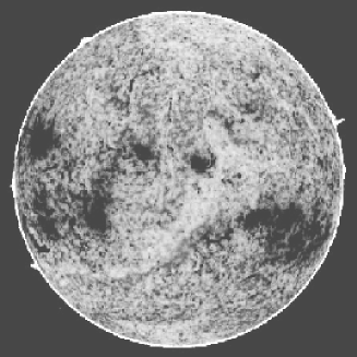
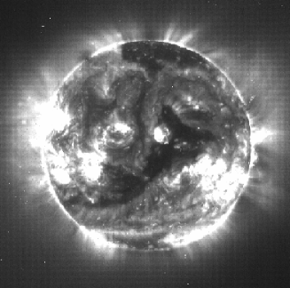
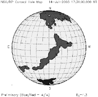
Figure 1.: KPVT He I 1083 nm spectroheliogram (top, left), EIT 19.5 nm Fe XII emission line image (top, right), the KPVT associated “hand-drawn” coronal hole image (bottom, left), and the automated detection coronal hole image (bottom, right) for July 14, 2003 at approximately 17 UT.

Using KPVT He I 1083 nm spectroheliograms and photospheric magnetograms, daily computer-assisted “hand drawn” (HD) coronal hole images by Karen Harvey and Frank Recely span from April 1992 through September 2003. In addition, they constructed coronal hole Carrington synoptic maps for the period between September 1987 and March 2002 (see Harvey & Recely 2002). Prior to these periods HD maps were drawn on photographic prints and incorporated in synoptic maps published in Solar Geophysical Data. The creation of the HD coronal hole images and synoptic maps is notably labor intensive, requiring iterative visual inspection of high resolution helium spectroheliograms and photospheric magnetograms. The production of HD coronal hole maps stopped with the conclusion of operation of the KPVT in September 2003. Unpublished HD daily and synoptic maps exist for periods back to 1974.

The motivation for developing an automated detection (AD) coronal hole algorithm is to create daily images and synoptic maps similar to the hand-drawn maps for the period between 1974 and 1992 using available KPVT data. In addition, the AD algorithm will be used to create coronal hole images using the daily SOLIS Vector SpectroMagnetograph (VSM) helium spectroheliograms and photospheric magnetograms. The SOLIS-VSM began synoptic observations in August 2003. Initially during the development of the AD coronal hole algorithm, only the helium equivalent width images were utilized, at various spatial scales and thresholds, with limited success (Henney & Harvey 2001). The critical addition for the detection recipe presented here is the inclusion of magnetograms in the analysis to determine the percent unipolarity of the candidate region (e.g. Harvey & Recely 2002) to avoid areas of polarity inversions and centers of supergranular cells that otherwise resemble coronal holes.

Other methods for detecting coronal holes include utilizing spectral line properties of He I 1083 nm (Malanushenko & Jones 2005) and multi-wavelength analysis (de Toma & Arge 2005). In future work, we plan to compare these methods in detail with the AD coronal hole algorithm presented here. The following sections outline the parameterizing of coronal holes (Section 2), the coronal hole detection recipe, along with a comparison with the HD coronal hole images and the creation of synoptic maps (Section 3).

2. Coronal Hole Parameters

The preliminary step in the development of the automated coronal hole detection algorithm outlined in the following section is to parameterize unique properties of coronal holes. This allows for general threshold limits to be set for the input data. The thresholds used to select coronal hole candidate regions are estimated using successive pairs of KPVT magnetogram and helium spectroheliogram data originally used to create the HD coronal hole maps. Using the coronal hole boundaries from the hand drawn images, the area of each coronal hole is projected into the corresponding average magnetogram and helium spectroheliogram image in heliographic coordinates.

Figure 2.: Coronal hole parameters, for the period between 1992 through 2003, verses latitude (left) and central meridian distance (CMD, right). The total number of holes (top), normalized helium 1083 nm equivalent width (EQW, middle), and mean percent unipolarity (bottom) are shown. The 1-$\sigma$ error for the values is delineated by the vertical lines. See text for discussion.

The average images are created with two consecutive observations weighted inversely by one plus the time difference between the observations in fractional days. The two images are averaged in heliographic coordinates sine-latitude and longitude, where the older image is rotated into the time reference frame of the most recent image. The KPVT data coverage for the period April 1992 through September 2003 includes 2,781 image pairs. For this period, the boundaries of 11,241 HD coronal holes were used to estimate the mean percent unipolarity for these regions relative to latitude and central meridian distance.

In Figure 2, the number of coronal holes (top), the normalized He I 1083 nm equivalent width (middle) and the mean percent unipolarity (bottom) are exhibited for the period between 1992 and 2003. The helium equivalent width is normalized by the median of all positive values, where the zero point is essentially the mean of the disk values excluding active regions and filaments. Note that for the KPVT helium equivalent width images the limb darkening is removed. For this period a greater number of coronal holes were detected in the southern hemisphere. The difference between the hemispheres could be a result of a delayed or slower migration of the holes to the southern polar region or possibly longer lived regions, since no attempt was made to avoid recounting long-lived regions. The greater number of detections on the eastern limb is most likely a result of false detections. For the normalized helium equivalent width and the mean unipolarity percentage shown in Figure 2, the dashed lines delineate the threshold used with the AD algorithm. In addition, provisional regions are allowed for the east limb where the magnetic information becomes sparse due to the time difference between observations that constitute the average magnetogram. The threshold for the percent unipolarity is lowered for regions within the central meridian distance band between -90 and -50 degrees (depicted by the dotted line in Figure 2).

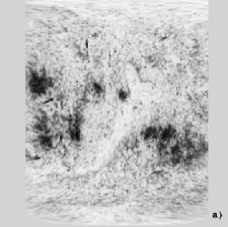
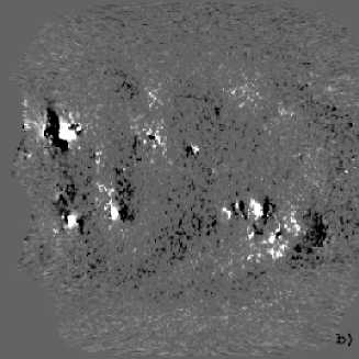
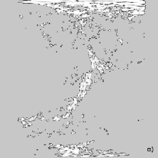
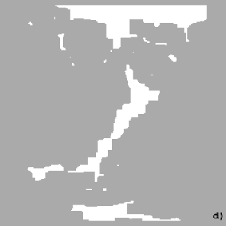
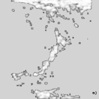
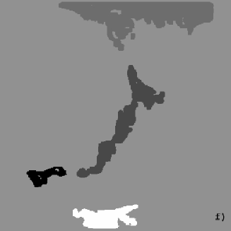
Figure 3.: Selected images throughout the automated coronal hole detection process are depicted: a) the initial average helium spectroheliogram in heliographic coordinates; b) the average magnetogram; c) after retaining only values from the image shown in a) above 0.10 of the median of the positive values; d) after applying the Close function; e) after applying the Open function; f) after removing small and low percentage unipolarity regions.

3. Automated Detection Recipe

The coronal hole detection process begins with a two-day average He I 1083 nm spectroheliogram and a two-day average photospheric magnetogram. The average images are created as discussed in the previous section. The helium image averaging assists in the detection of coronal holes by taking advantage of the low intrinsic network contrast within coronal holes (e.g. Harvey & Recely 2002). The weighted average images are trimmed on the east and west limb regions for unsigned central meridian distances greater than 70 degrees (see Figure 3a and 3b).

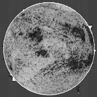
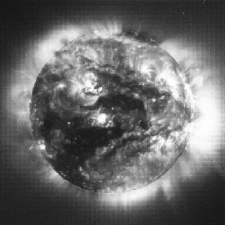
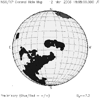
Figure 4.: An example when the HD (bottom, left) and AD (bottom, right) coronal hole images disagree. KPVT He I 1083 nm spectroheliogram (top, left), and EIT 19.5 nm Fe XII emission line image (top, right) observed on March 12, 2003 are also shown.

Starting with the average helium image, the first step is to retain only values above $1/10$ the median of positive values (based on the mean values shown in Figure 2). After removing the negative values, the candidate coronal hole regions become clearly visible (see Figure 3c). The next two steps are to spatially smooth the remaining positive values and set all positive value pixels to a fixed value. The resultant image is then smoothed with the morphological image analysis function Close (e.g. Michielsen & De Raedt 2001) using a square kernel function as the shape-operator. Shown in Figure 3d, the Close function fills the gaps and connects associated or nearby regions to define the areas of the coronal hole candidates. The regions that are too small to be coronal holes are then removed (see Harvey & Recely 2002). The spatial image pixel positions of non-zero spatial points of the resultant image (e.g. Figure 3d) are used to fill the corresponding pixels in the image that was created after the first step (e.g. Figure 3c) with large values (e.g. $10^{4}$). After being spatially smoothed, the large values result in the filling of small gaps and holes. The resultant image is then smoothed with the morphological image analysis function Open (e.g. Michielsen & De Raedt 2001), where the Open function removes small features while preserving the size and shape of larger regions (see Figure 3e). For more discussion on morphological image analysis and standard algorithms for segmenting images see Jähne (2004).

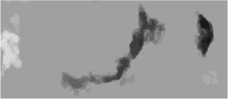
Figure 5.: Subregion of an automated coronal hole synoptic map for Carrington rotation 2005. The gray-scale reflects the polarity (positive and negative are represented by white and black respectively) and the number of coronal hole detections at a given latitude and longitude. The central region is the same coronal hole exhibited in Figure 1 and 3.

The primary goal of the steps so far has been to consolidate and define the boundaries of candidate coronal hole regions. The next step is to use the average magnetic image data to determine the percentage of unipolarity of each candidate region. Candidate regions that have a percentage of unipolarity lower than the thresholds (delineated by the dashed lines in Figure 2) are removed. The final step is to number the coronal hole candidates and apply the sign of the region polarity (e.g. Figure 3f). Candidate regions with mean unipolarity values that fall within the dashed and dotted lines depicted in Figure 2 are considered provisional. These regions are distinguished in the final output image by adding a fractional value (e.g. 0.5) to the region number value of the image pixels for the given coronal hole area.

3.1. Coronal Hole Map Comparison

In general the coronal hole candidate regions detected by the AD algorithm agree well with the HD images. For the 11 years compared, the automated coronal hole areas have approximately 3% less area than the hand-drawn regions between -50 through 90 degrees latitude. The difference increases for the latitude band between -90 and -50 degrees. However, the increase is believed to be the result of incomplete observations used in the average images (i.e. the KPVT full-disk observations always began in the north). Comparisons between the HD and AD coronal hole images are shown in Figures 1 and 4. The two images agree for the July 14, 2003 example shown in Figure 1. However, comparisons with only the HD maps have the limitation of not comparing directly with coronal measurements. Figure 4 highlights this difficulty. For this example, the AD map is in better agreement with the EIT image. A detailed comparison with other coronal hole detection methods (e.g. de Toma & Arge 2005; Malanushenko & Jones 2005) is planned. These comparisons will undoubtedly result in further refinement to the presented AD algorithm.

3.2. Coronal Hole Synoptic Maps

In addition to creating coronal hole images, these individual images are combined to create synoptic maps for fixed Carrington rotation or daily synoptic maps. Each pixel value of the synoptic map represents the number of detections that a coronal hole is observed for that location. A subregion from an example Carrington map is shown in Figure 5. These maps reflect the estimated coronal hole boundary variations as a result of temporal evolution of the region in addition to the quality of the detection. The new synoptic maps will be publicly available via the NSO digital library along with the daily AD coronal hole images.

4. Acknowledgments

The coronal hole data used here was compiled by K. Harvey and F. Recely using National Solar Observatory (NSO) KPVT observations under a grant from the National Science Foundation (NSF). NSO Kitt Peak data used here are produced cooperatively by NSF/AURA, NASA/GSFC, and NOAA/SEL. The EIT images are courtesy of the SOHO/EIT consortium. This research was supported in part by the Office of Naval Research Grant N00014-91-J-1040. The NSO is operated by the Association of Universities for Research in Astronomy, Inc. under cooperative agreement with the NSF.

References

- Andretta & Jones (1997) Andretta, V., & Jones, H. P. 1997, ApJ, 489, 375
- Arge et al. (2004) Arge, C. N., Luhmann, J. G., Odstrcil, D., Schrijver, C. J., Li, Y. 2004, Journal of Atmospheric and Solar-Terrestrial Physics, 66, 1295
- Bohlin (1977) Bohlin, J. D. 1977, in Coronal Holes and High Speed Wind Streams, ed. J. B. Zirker, (Colorado:CAU Press), 27
- Harvey & Sheeley (1977) Harvey, J. W., & Sheeley, N. R., Jr. 1977, Solar Physics, 54, 343
- Harvey & Livingston (1994) Harvey, J. W., & Livingston, W. C. 1994, in IAU Symp. 154, Infrared Solar Physics (Dordrecht:Kluwer), 59
- Harvey & Recely (2002) Harvey, K. L., & Recely, F. 2002, Solar Physics, 211, 31
- Henney & Harvey (2001) Henney, C. J., & Harvey, J. W. 2001, at the American Geophysical Union, Spring Meeting, SP51B-03
- Jähne (2004) Jähne, B. 2004, Practical Handbook on Image Processing for Scientific and Technical Applications, 2nd ed., (Boca Raton:CRC Press)
- Malanushenko & Jones (2005) Malanushenko, O. V., & Jones, H. P. 2005, Solar Physics, in press
- Michielsen & De Raedt (2001) Michielsen, K., & De Raedt, H. 2001, Physics Reports, 347, 461
- de Toma & Arge (2005) de Toma, G., & Arge, C. N., these Proceedings
- Zirker (1977) Zirker, J. B. 1977, in Coronal Holes and High Speed Wind Streams, ed. J. B. Zirker, (Colorado:CAU Press), 1