The Non-Parametric Model for Linking Galaxy Luminosity with Halo/Subhalo Mass: Are First Brightest Galaxies Special?

Abstract

We revisit the longstanding question of whether first brightest cluster galaxies are statistically drawn from the same distribution as other cluster galaxies or are “special”, using the new non-parametric, empirically based, model presented in Vale & Ostriker (2006) for associating galaxy luminosity with halo/subhalo masses.

We introduce scatter in galaxy luminosity at fixed halo mass into this model, building a conditional luminosity function (CLF) by considering two possible models: a simple lognormal and a model based on the distribution of concentration in haloes of a given mass. We show that this model naturally allows an identification of halo/subhalo systems with groups and clusters of galaxies, giving rise to a clear central/satellite galaxy distinction, obtaining a special distribution for the brightest cluster galaxies (BCGs).

Finally, we use these results to build up the dependence of BCG magnitudes on cluster luminosity, focusing on two statistical indicators, the dispersion in BCG magnitude and the magnitude difference between first and second brightest galaxies. We compare our results with two simple models for BCGs: a statistical hypothesis that the BCGs are drawn from a universal distribution, and a cannibalism scenario merging two galaxies from this distribution. The statistical model is known to fail from work as far back as Tremaine & Richstone (1977). We show that neither the statistical model nor the simplest possibility of cannibalism provide a good match for observations, while a more realistic cannibalism scenario works better. Our CLF models both give similar results, in good agreement with observations. Specifically, we find $<m_{1}>$ between -25 and -25.5 in the K-band, $\sigma(m_{1})\sim 0.25$ and $<\Delta_{12}>$ between 0.6 and 0.8, for cluster luminosities in the range of $10^{12}$ to $10^{13}h^{-2}{\rm L_{\odot}}$.

1 Introduction

The nature of brightest cluster galaxies (BCGs) has long been a subject of interest and much debate (Peebles, 1968; Sandage, 1972; Dressler, 1978). In particular, investigators have asked whether their origin is statistical or special in nature, that is, whether they follow a special distribution independent of the fainter galaxies in the cluster, or on the contrary, they are merely the extreme values of the same global distribution derived for all cluster galaxies.

On the theoretical side, there has been renewed interest in this subject with recent studies of the relation between galaxies and their dark matter haloes from a theoretical, statistical point of view, involving the study of the distribution of the galaxy population through different haloes while bypassing the complications of the physics of galaxy formation (e.g., Berlind & Weinberg 2002; Vale & Ostriker 2004; Tasitsiomi et al. 2004; Yang et al. 2005; Zehavi et al. 2005; Zheng et al. 2005; Cooray 2006; Conroy, Wechsler & Kravtsov 2006; van den Bosch et al. 2006). Since these involve populating dark matter haloes with galaxies, they usually lead to a distinction between central and satellite galaxies. This in turn has lead to, in many of these works, central galaxies being treated separately from the rest, and therefore having a distinct distribution, with consequences visible, for example, in the luminosity function. Some of these studies have in fact looked at some specific BCG-related properties of clusters, like the magnitude gap (e.g., Milosavljević et al. 2006; van den Bosch et al. 2006).

In the past, observational studies which have focused on this issue (Tremaine & Richstone, 1977; Hoessel, Gunn & Thuan, 1980; Schneider, Gunn, & Hoessel, 1983; Bhavsar & Barrow, 1985; Hoessel & Schneider, 1985; Bhavsar, 1989; Postman & Lauer, 1995; Bernstein & Bhavsar, 2000) have been hindered by the limited numbers of high luminosity galaxy observations available, since the strongly declining nature of the bright end of the luminosity function requires having very large samples to obtain significant numbers of high luminosity galaxies. Due to this, these studies were mostly inconclusive when it came to answer the question of whether BCGs were statistical or special in nature, although many works hinted at the latter. More recently, the advent of large scale surveys such as the 2dF Galaxy Redshift Survey or the Sloan Digital Sky Survey (SDSS), has motivated plentiful, ongoing work on this subject (e.g., Lin, Mohr & Stanford 2004; Lin & Mohr 2004; Loh & Strauss 2006; Bernardi et al. 2006; von der Linden et al. 2006).

This issue is in large part motivated by the fact that, observationally, BCGs do look different from other galaxies. They usually sit at the centre of the cluster, and tend to be considerably brighter than the remaining cluster members. The most striking case is cD galaxies, found in the centre of rich clusters and which dominate their satellites in both size and brightness, while having a characteristically distinct morphology and surface brightness distribution (e.g., Binggeli, Sandage & Tammann 1988). Likewise, cD galaxies tend to be brighter than what would be expected from the bright end of the cluster galaxy luminosity function. In fact, it has been observed that, when analyzing composite luminosity functions of cluster galaxies, the most luminous of them form a hump at the bright end (e.g., Colless 1989; Yagi et al. 2002; Eke et al. 2004). Yet, at the same time, there is little variation in magnitude among them (Hoessel & Schneider, 1985; Postman & Lauer, 1995; Bernardi et al., 2006; von der Linden et al., 2006). This ties in with the fact that the luminosity of BCGs is expected to vary only slowly with increasing cluster luminosity (Lin & Mohr 2004; see also the results for the mass luminosity relation of central galaxies in Vale & Ostriker 2006).

In order to try to answer this problem from available observational data, two different indicators have been considered. One is the shape of the overall distribution of the magnitude of BCGs. If BCGs are merely the extreme cases of a general distribution applicable to all cluster galaxies, then it is expected that results from extreme value theory in statistics apply, predicting a resulting distribution shaped like the Gumbel distribution (Bhavsar & Barrow, 1985; Bernstein & Bhavsar, 2000). On the other hand, if BCGs are considered a special, distinct type of galaxy, then some particular distribution is to be expected, such as a Gaussian (Postman & Lauer, 1995) or lognormal. Some studies have also raised the possibility that it could be actually a combination of the two, probably depending on the type of cluster (Bhavsar, 1989; Bernstein & Bhavsar, 2000).

The other property studied is the ratio $r=\Delta_{12}/\sigma_{1}$, where $\Delta_{12}$ is the average magnitude difference between the first and second brightest galaxies, and $\sigma_{1}$ the dispersion in the magnitude of the first brightest galaxy. It is possible to prove the powerful conclusion (Tremaine & Richstone, 1977) that, if all galaxies are drawn from the same statistical distribution, regardless of its exact form, then $r\leq 1$. Observational results give a value for $r$ around 1.5 (e.g., Lin & Mohr 2004; Loh & Strauss 2006), which would exclude this possibility.

This has led to the study of possible alternative scenarios for the formation of BCGs, in order to account for their special nature. One such is galactic cannibalism, initially proposed by Ostriker and collaborators (Ostriker & Tremaine, 1975; Ostriker & Hausman, 1977; Hausman & Ostriker, 1978). Such a scenario is akin to taking the above case of having all galaxies drawn from the same distribution, but then merging the brightest of them with one or more of the others. From this simplistic model of the process, it is easy to see that this mechanism would help to solve the above problem, mostly by increasing the value of $\Delta_{12}$ as the luminosity of the first brightest galaxy is driven up by the mergers and the brightness of the surviving second brightest galaxy declines as luminous galaxies are merged out of existence.

In the present paper, we explore this issue in light of the non-parametric model for the mass luminosity relation presented in Vale & Ostriker (2006) (hereafter paper I; see also Vale & Ostriker 2004). The basic idea behind the non-parametric model is to adopt the simple proposition that more luminous galaxies are hosted in more massive haloes/subhaloes. No attempt at physical modelling is made and the association is made simply by matching one-to-one the rank ordered observational list of galaxies with the rank ordered computed list of haloes/subhaloes. We here extend this model by introducing scatter into it, and also by considering possible effects on the total disruption of some subhaloes into the total luminosity related to the halo.

As is the case in HOD models (e.g., Berlind & Weinberg 2002; Zehavi et al. 2005; Zheng et al. 2005), this model naturally gives rise to a separation between central and satellite galaxies, by associating the former with the parent halo itself and the latter with the subhaloes associated with it. We analyze this issue in more detail, studying how it affects the cluster galaxy luminosity function and gives rise to a bright end bump caused by the central galaxies. We then develop a model for the BCG luminosity distribution. Since the halo in fact arises from the union of subhaloes this non-parametric model is a statistically well defined variant of the cannibalism scenario.

This paper is organised as follows: in section 2, we give a brief summary of the non-parametric model relating galaxy luminosity with halo/subhalo mass presented in paper I, and introduce a simple recipe for checking the contribution of destroyed subhaloes to the halo mass, and how this changes our estimate of the total luminosity. In section 3, we introduce scatter into the non-parametric model by building a conditional luminosity function, where we consider two possibilities for it, either a simple lognormal shape or a better motivated approach involving the distribution of concentration for haloes of a given mass. In section 4, we explore more indepth how the model gives rise to a central/satellite galaxy separation, and show how this impacts the cluster galaxy luminosity function. In section 5, we build up a model for the distribution of cluster galaxies, based on the mass-luminosity relation and the halo/subhaloes separation which underpins it. In section 6, we present simple models to account for another two possible origins for the BCG distribution: first, we consider that all cluster galaxies are drawn from the same distribution; then we take a simple model for cannibalism, by merging two of the galaxies (the brightest plus one other) in the first example. Finally, in section 7 we present the results of all models for the average magnitude of first and second brightest galaxies as well the dispersion of the former as a function of cluster luminosity. We then compare these results with observations.

Throughout we have used a concordance cosmological model, with $\Omega_{m}=0.24$, $\Omega_{\Lambda}=0.76$, $h=0.735$ and $\sigma_{8}=0.74$ (Spergel et al., 2006).

2 The Mass-luminosity relation

The work presented below is based on the non-parametric model for relating galaxy luminosity with halo/subhalo mass presented in paper I. The basic idea is that more massive haloes/subhaloes have deeper potential wells and will thus accrete more gas and subsequently will have more luminous galaxies forming within them. In effect, we take the relation between galaxy luminosity and halo/subhalo mass to be one to one and monotonic. An additional extra ingredient is necessary to maintain this approximation in the framework of the model, since subhaloes lose mass to the parent halo after accretion due to tidal interactions. Alternatively put, a halo is not simply the sum of the identifiable subhaloes within it due to tidal stripping. Therefore, we need to account for the mass of the subhaloes not at present, but that which they had at the time of their merger into the parent. The relation between mass and luminosity is then obtained statistically by matching the numbers of galaxies with the total number of hosts, that is, haloes plus subhaloes through their distributions.

The halo abundance is given by the usual Sheth-Tormen mass function (Sheth & Tormen, 1999):

$$n_{h}(M)dM=A\Big{(}1+\frac{1}{\nu^{2q}}\Big{)}\sqrt{\frac{2}{\pi}}\frac{\rho_{m}}{M}\frac{d\nu}{dM}{\rm exp}\Big{(}-\frac{\nu^{2}}{2}\Big{)}dM\,,$$ (1)

with $\nu=\sqrt{a}\frac{\delta_{c}}{D(z)\sigma(M)}$, $a=0.707$, $A\approx 0.322$ and $q=0.3$; as usual, $\sigma(M)$ is the variance on the mass scale $M$, $D(z)$ is the growth factor, and $\delta_{c}$ is the linear threshold for spherical collapse, which in the case of a flat universe is $\delta_{c}=1.686$, with a small correction dependent on $\Omega_{m}$ ($\delta_{c}=1.673$ for $\Omega_{m}=0.24$).

Following the discussion in paper I, we will assume a very simple model for the subhalo mass distribution within the parent. In terms of their original, pre-accretion mass, we assume that the subhalo distribution is given by a simple Schechter function:

$$N(m|M)dm=A(M)(m/\beta M)^{-\alpha}{\rm exp}(-m/\beta M)dm/\beta M\,,$$ (2)

where the cutoff parameter $\beta=0.5$ serves to insure that no subhalo was larger than half the present mass of the parent (otherwise it would, by definition, be the parent). The slope $\alpha=1.9$ is set to the same value as is generally found for the present day subhalo mass function in simulations (e.g., Gao et al. 2004; Weller et al. 2005; van den Bosch, Tormen & Giocoli 2005; Zentner et al. 2005; Shaw et al. 2006). The normalization $A(M)=1/\beta[\Gamma(2-\alpha)-\Gamma(2-\alpha,1)]$ is set so that the total mass originally in subhaloes corresponds to the present day mass (where the integration is done to an upper limit of $0.5M$). This approximation potentially ignores the problem of total disruption of some of the merged subhaloes, as can occur for example in the case of major mergers, by assuming that all of these subhaloes are still present and that therefore the total fraction of mass originally in subhaloes is one. In Vale & Ostriker (2006), we showed that as long as this fraction is close to one, then the resulting mass luminosity relation is similar, with both number of satellites in a halo and their total luminosity decreasing slightly. From the study of simulation results it is still not completely clear how to treat this complex issue, and no simple analytical models are available, so we explore a simple recipe to better account for this problem in the context of our model in section 2.1.

The galaxy distribution is given by the luminosity function. This is given by the usual Schechter function fit:

$$\phi_{obs}(L)dL=\phi_{*}\Big{(}\frac{L}{L_{*}}\Big{)}^{\alpha}{\rm exp}\Big{(}-\frac{L}{L_{*}}\Big{)}\frac{dL}{L_{*}}\,.$$ (3)

The values of the parameters will depend on the waveband used. In this paper, we use mostly the K-band luminosity function from the 2MASS survey, with parameters given by $\alpha=-1.09$, $\phi_{*}=1.16\times 10^{-2}h^{3}{\rm Mpc^{-3}}$ and $M_{*}-5{\rm log}h=-23.39$ (Kochanek et al., 2001). For comparison, we also obtain the $b_{J}$-band 2dF survey, with $\alpha=-1.21$, $\phi_{*}=1.61\times 10^{-2}h^{3}{\rm Mpc^{-3}}$ and $M_{*}-5{\rm log}h=-19.66$ (Norberg et al., 2002). Also note that we are in fact extending these fits as necessary, including beyond the magnitude interval in which they were obtained.

The basic mass-luminosity relation can then be obtained from these ingredients by a counting process, matching the numbers of galaxies at a given luminosity to the total number of hosts at a given mass:

$$\int_{L}^{\infty}\phi(L)dL=\int_{M}^{\infty}(n_{h}(M)+n_{sh}(M))dm\,,$$ (4)

where the host contribution is separated into a halo term, $n_{h}(M)$, and a subhalo term obtained by summing up all the subhaloes at that mass, $n_{sh}(m)=\int_{0}^{\infty}N(m|M)n_{h}(M)dM$. An average relation between host mass and galaxy luminosity can then be built through this process, with results that match well with observations (see paper I for a detailed analysis). The resulting relation can be well fit by a double power law of the type:

$$L_{ref}(M)=L_{0}\frac{(M/M_{0})^{a}}{[1+(M/M_{0})^{bk}]^{1/k}}\,,$$ (5)

where the differents parameters are shown in table 1; mass is in units of $h^{-1}{\rm M}_{\odot}$, luminosity in $h^{-2}{\rm L}_{\odot}$. The fit was done in the mass range $10^{11}$ ($3\times 10^{10}$ in the $b_{j}$ band case) to $3\times 10^{15}$ $h^{-1}{\rm M}_{\odot}$.

	K-band	$b_{J}$-band
$L_{0}$	$1.37\times 10^{10}$	$4.12\times 10^{9}$
$M_{0}$	$6.14\times 10^{9}$	$1.66\times 10^{10}$
$a$	21.03	6.653
$b$	20.74	6.373
$k$	0.0363	0.111

Table 1: Fit parameters for the mass-luminosity relation.

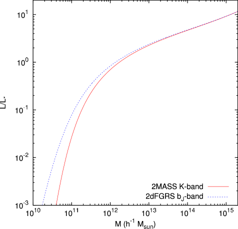
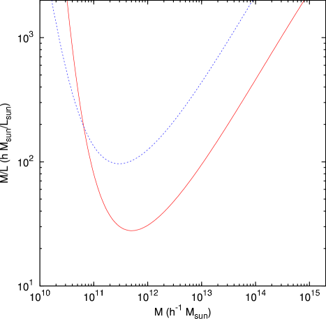
Figure 1: Mass-luminosity relation as obtained using the non-parametric model, in the K- and $b_{J}-$ bands. Upper pannel shows galaxy luminosity normalized to the characteristic luminosity, $L^{*}$, of each band; lower pannel shows the corresponding mass-to-light ratio.

Figure 1 shows the results for the luminosity of a single galaxy as a function of the mass of the hosting halo/subhalo, together with the corresponding mass-to-light ratio. Shown are curves for both K- and $b_{J}$ bands. We caution that the results for the latter band should be treated with some reserve. This counting method is not entirely adequate to get the mass-luminosity relation in the blue, due to complications arising from recent star formation, although it is still interesting to compare the differences obtained from using two different luminosity functions.

2.1 Destroyed subhaloes and the subhalo mass fraction

As mentioned, a potentially important correction to the non-parametric model in paper I is to account for subhaloes which have been completely destroyed. The study of this evolution of the subhalos and their eventual destruction, with the subsequent merger (or not) of their galaxy with the central one, is a very interesting topic by itself, which is still not completely understood but which is essential to a complete understanding of the formation of BCGs. However, such a detailed look at this question is beyond the scope of the present paper; here, we are merely interested in a simple model to account for how much mass was in these destroyed subhalos, to correct the normalization of our original subhalo mass function.

Our scheme is based on the fact that most of the luminosity of the central galaxy is built up by merging with the satellite galaxies brought in by these subhaloes. In other words, the central (BCG) optical galaxy is made up of the galaxies that have been ”merged away” – disappeared from the original distributions. This is consistent with what is known of the size, shape and colour properties of central galaxies. We therefore assume that the fraction of mass in these destroyed subhalos (with respect to the total halo mass), is given by the ratio of the central galaxy luminosity to the total luminosity of the halo:

$$f_{dest}=\frac{m_{dest}}{M}=\frac{L_{cent}}{L_{total}}\,.$$ (6)

For a given $L(M)$ relation, which sets the luminosity of both the central and satellite galaxies as a function of the halo/subhalo mass, the previous equation can then be solved for $f_{dest}$ as a function of halo mass, since the total luminosity is going to be a function of only it and the total mass: $L_{total}=L_{cent}(M)+(1-f_{dest})L_{sat,max}(M)$, where $L_{sat,max}$ is the maximum contribution of the satellites for when $f_{dest}=0$. This is given by:

$$L_{sat,max}(M)=\int_{0}^{0.5M}L_{ref}(m)N(m|M)dm\,.$$ (7)

The upper pannel of figure 2 shows the destroyed mass fraction as a function of halo mass for our base mass-luminosity relation, given by equation (5), while the bottom pannel shows the effect on the total luminosity. As can be seen, this is most pronounced at the lower end of the mass scale shown, and becomes small enough to have little effect at high mass.

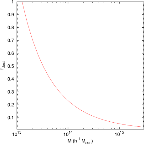
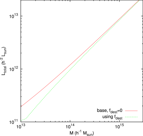
Figure 2: Upper pannel: total mass in subhaloes which have been completely disrupted, as a fraction of the total halo mass. Bottom pannel: total luminosity as a function of halo mass with or without using the fraction of mass in destroyed subhaloes shown in the upper pannel. Results are for the K-band, using the base mass-luminosity relation of equation (5).

There are two additional factors that need to be noted. First, the introduction of this term can also have an effect on the actual mass-luminosity relation, since we are using a counting method to obtain it. However, for the mass range we are interested in, the number counts are dominated by the central galaxies and will therefore not be affected (see section 4). Likewise, the only haloes capable of hosting subhaloes large enough to be counted in this range are the most massive ones, for which the effect is smallest (see section 3). Secondly, in principle, this approach will also depend on the exact form of the mass-luminosity relation. However, for the small deviations from the base relation we will be considering in this paper, the effect on the total luminosity is small, since the variation to the base relation will be greatest at higher mass, where this effect is smallest. We will therefore, for simplicity, use this one result throughout the paper.

Finally, it needs to be stressed that this is just a very simple approximation. The calculated factor is applied to the whole subhalo mass fraction as a correction to the normalization, without taking into account a possible dependence on subhalo mass. In particular, the situation with very low mass subhaloes is very uncertain in this scheme, since they are expected to be very faint, and have therefore very little weight in the sum of the total luminosity, while they can contribute an important fraction of the mass. Another important point is that in principle the luminosity of the galaxies that were contained in the destroyed subhaloes should be added to the central galaxy luminosity, since under this scheme we are assuming that these are merging. In practice, though, the light in these destroyed subhaloes is going to be small in comparison with the BCG in this model, since the largest fraction of destroyed subhaloes occurs for less massive haloes where the BCG is dominant. For simplicity, we will here ignore this contribution.

3 Introducing scatter

3.1 The conditional luminosity function

In the context of the present paper, we need a more detailed model than the one described previously. Most importantly, it needs to include some kind of scatter in the mass-luminosity relation. Naturally, we expect that not all galaxies in hosts of the same mass will have the same luminosity. To capture this, we introduce a dispersion around the average relation describe above. We use the conditional luminosity function (CLF) formalism introduced by Yang et al. (2003) (see also van den Bosch et al. 2006 and references therein) and by Cooray and collaborators (e.g., Cooray & Milosavljević 2005a; Cooray 2006 and references therein). This consists of replacing a deterministic mass-luminosity relation, like the one in equation (5), with a distribution of luminosity around an average value for any given halo mass, $\phi_{CLF}(L|M)dL$, which represents the probability of having a galaxy of luminosity $L$ in a halo of mass $M$. Note that here we are only applying this to the central galaxy in any given halo, since that is the important one for the study of BCGs; the distribution of satellite galaxies we draw directly from the distribution of subhalo masses.

An important point is that this CLF must, by definition, match the observed luminosity function when it is integrated over all haloes, i.e. $\int_{0}^{\infty}\phi_{CLF}(L|M)n(M)dM=\phi(L)$, where $n(M)$ is the halo mass function, $\phi(L)$ the observed luminosity function and $L$ should only be considered in the range where the haloes dominate the number of hosts (i.e., at high luminosity, which is precisely the range we are interested in when looking at BCGs;otherwise, we would also need to account for subhalo contribution). The introduction of scatter then leads to a problem with the mass-luminosity relation derived from the counting method, however. As noted by Tasitsiomi et al. (2004), the fact that the mass function is decreasing with increasing mass causes an effect similar to the Malmquist bias: for any given mass bin, more objects are scattered into it from lower mass bins than are scattered out of it. If we then take our base mass-luminosity relation to be the average one in the CLF distribution, because of this effect we will end up with a calculated luminosity function that greatly overestimates the abundance of very bright galaxies when compared to the observed one.

To get the correct matching to the observed luminosity function, it is then necessary to modify the average mass-luminosity function we take for the basis of the CLF. This is achieved by introducing an additional term, of the form:

$$L(M)=L_{ref}(M)(1+M/M_{s})^{a}\,,$$ (8)

where $L_{ref}(M)$ refers to the base mass-luminosity relation of equation (5). In practice, $a$ is going to be negative since we need to lower the luminosity corresponding to any given high-mass halo in order to drive the value of our calculated luminosity function down.

There is one final, potentially important point about this issue: once scatter is introduced, care must be taken when looking at the calculated average mass-luminosity relation. In our approach, the average luminosity at fixed mass needs to go down, relative to the scatter-less case or, looking at it the opposite way, the same average luminosity is obtained for higher mass haloes. This is due to the fact that, when considering the CLF, we are doing the binning by mass (or more precisely, taking the conditional variable in the distribution to be the mass). If we had instead binned by luminosity, the effect of introducing scatter would have been the opposite: the average mass correspoding to a given luminosity would instead have gone down. This is to be expected and is just a statistical effect of the two different ways in which the conditional function can be defined. It does however mean that care must be taken when comparing results of different authors to look at how the binning was done in each case.

In this paper we will consider two different models for the CLF of the central galaxy: a simpler model where we assume the distribution is lognormal, but where we are left with a free parameter in the scatter introduced; and a more complicated one based on the distribution of concentrations at a given halo mass, which fully motivates the introduction of scatter in the CLF without any free parameters. For the satellite galaxies we will use the same modified mass-luminosity relation as well, since these were central galaxies within their own independent haloes prior to merging, so it is reasonable to expect the same effects to apply to them. From semi-analytical modelling, it has been shown that this is a good approximation, although a more careful treatment shows a slightly different relation for sattelites than for central galaxies (Wang et al., 2006). But note that, when doing analytical calculations, using the subhalo mass function already introduces a form of distribution for the subhaloes as well (in that the mass of a given subhalo can be drawn from it, see section 5.1 for further discussion).

3.2 Lognormal model

The simplest CLF model we consider is to assume it has a lognormal form. This is similar to what was done previously by other authors (Cooray & Milosavljević, 2005a; Cooray, 2006), and such a form seems a good match to the distribution of stellar mass obtained in semi-analytic modelling (Wang et al., 2006). The problem with this approach is that there is no a priori reason to assume any specific value for the dispersion. Furthermore, this value is linked to the modified mass-luminosity relation of equation (8), so it needs to be defined in some way in order to determine the latter. We do this by determining which value of the dispersion leads to an average luminosity as a function of mass which best fits observational values. For simplicity, we will consider that the value of the dispersion, $\sigma$, is constant and independent of mass. Since we are only interested in the bright end, where we expect central galaxies to dominate, and these are known to have only a small scatter in luminosity (e.g., Postman & Lauer 1995; Bernardi et al. 2006), this is quite likely a good approximation. Semi-analytical modelling also shows that scatter in stellar mass is only a weak function of halo mass (Wang et al., 2006).

The luminosity $L$ of a galaxy in a host of mass $M$, is then given by a lognormal distribution of the type:

$$\phi_{CLF}(L|M)dL=\frac{1}{\sqrt{2\pi}\sigma_{LN}L}{\rm exp}\Big{(}-\frac{({\rm ln}[L/L_{0}(M)]+\sigma_{LN}^{2}/2)^{2}}{2\sigma_{LN}^{2}}\Big{)}dL\,,$$ (9)

where $L_{0}(M)$ is some average luminosity for a host of mass $M$ (discussed further below), and $\sigma$ is the dispersion in the normal logarithm of the luminosity. Note that there is some confusion in the literature over the exact form defined for the lognormal distribution. First, it is necessary to pay attention to whether the distribution is in the natural logarithm or base 10 logarithm of the variable; the quoted value of $\sigma$ will be different in the two cases for the same distribution. Secondly, the way we have defined it in equation (9), the average luminosity is given by $L_{0}(M)$. This is due to the second term in the denominator of the exponential term, which not all authors include; if it is omitted, $L_{0}$ would not be the average luminosity.

The difficulty with using an approach such as this is that we are left with two unknowns we need to determine, the reference luminosity function $L_{0}$ and the dispersion $\sigma$. The only condition we can impose on this distribution is that, when integrated over all hosts, the resulting luminosity function must match the observed one. Fitting this calculated luminosity function to the observed one then allows us to relate the two parameters we have when we take $L_{0}=L(M)$ from equation (8), $a$ and $M_{s}$, to the scatter $\sigma$. However, this still leaves us with one free parameter which we cannot otherwise specify. In order to address this problem, we determine which value of the scatter gives us an average luminosity as a function of mass that best fits the observed data. Since our original mass-luminosity relation was already quite a good fit to the data (see paper I), we must necessarily have only a small correction to it (i.e., a small value of $a$), which in turn implies a small value for the scatter, which is qualitatively in good agreement with observations (see further discussion in section 7).

3.3 Concentration model

The other model for the CLF of BCGs we consider is based on the variation of the concentration of haloes with the same mass. The basic idea behind this is that the distribution of concentration in same mass haloes will lead to different mass in the inner region of the halo where the galaxy will be present; the luminosity of the hosted galaxy will then simply be proportional to this mass. In practice, we calculate the mass-to-light ratio of this inner region, for the average concentration and with an average luminosity given by equation (8), and then calculate the change in luminosity as the concentration changes by assuming that the mass-to-light ratio is fixed (observationally, it has been noted that the dynamical mass-to-light ratio of BCGs is almost constant, e.g. von der Linden et al. 2006). This then gives us the BCG luminosity as a function of both concentration and halo mass.

Although the model is conceptually simple, the details are problematic. The main issue is to determine what exactly is this inner region and how to calculate its mass. The most obvious solution, taking quoted values from the literature for BCG radius and its dependence on luminosity, is not really satisfactory since these are most often determined from isophotal limits and in the case of cD galaxies it would be necessary to further consider whether to include the envelopes; also, it is natural to assume that the actual region of influence for the dark matter is more extensive than the visible galaxy. Other options such as some parameter from the dark matter structure, run into the problem of motivating what exactly it should be.

In the end, after checking the results of several different possible models, we concluded that the one that has the best motivation and also gives the best results is to calculate the inner region mass by using a weighting function based on the luminosity profile of the BCGs.

Since we just require it to make our weighting function, for simplicity we assume that the luminosity profile of BCGs can be universally fit by a Sersic profile:

$$I(r)=A\,exp(-b_{n}[(r/r_{e})^{1/n}-1])\,,$$ (10)

where $A$ is a normalization factor, and $\Gamma(2n)=2\gamma(2n,b_{n})$, where $\Gamma(2n)$ is the gamma function and $\gamma(2n,x)$ the incomplete gamma function; this can be well approximated by $b_{n}\approx 2n-0.327$ (Capaccioli, 1989). It is know that there is a correlation between the profile parameters $n$ and $r_{e}$, and also between $r_{e}$ and the galaxy luminosity $L$, although the correlation between $n$ and $L$ is very weak (e.g., Graham et al. 1996). For simplicity, we will assume that we can relate both parameters to the galaxy luminosity; although in practice this is not really true, for our purposes here it is a sufficient, if rough, approximation. Based on results from the literature (Graham et al., 1996; Lin & Mohr, 2004), we use the following relations:

$$n=2.8694{\rm log}(r_{e})+2.0661\,,$$ (11)

$${\rm log}(r_{e})=0.9523{\rm log}(L)-9.1447\,,$$ (12)

where $L$ is the K-band luminosity; these are similar to what is reported by other authors (e.g., Bernardi et al. 2006). Our weighting function is then given not by the actual profile, but rather the integration factor for the luminosity, $w(r)=rI(r)$, and the normalization $A$ chosen so that $\int_{0}^{r_{vir}}w(r)dr=1$. Finally, the inner region mass is simply obtained by integrating the mass density times the weighting function:

$$M_{inner}=\int_{0}^{r_{vir}}4\pi r^{2}w(r)\rho(r)dr\,.$$ (13)

We use the usual NFW profile for the density (Navarro, Frenk, & White, 1997),

$$\rho=\frac{\rho_{1}}{x(x+1)^{2}}\,,$$ (14)

where $x=r/r_{s}$, with $r_{s}=r_{vir}/c_{vir}$ and the virial radius is $r_{vir}=(3M/4\pi\Delta_{vir}\bar{\rho})^{1/3}$ and $\Delta_{vir}=387$; $\rho_{1}$ is normalized to give the halo mass at the virial radius.

For the concentration distribution, we take the model of Bullock et al. (2001) (see also Macciò et al. 2006, who get similar results). This relates the average concentration of a halo of mass $M$ with the scale factor at its collapse, $a_{c}$, given by:

$$\sigma(fM)=\frac{\delta_{c}}{D(a_{c})}\,,$$ (15)

where $\sigma$ is, as usual, the variance of the linearly extrapolated power spectrum of perturbations, $D(a)$ is the growth factor and $\delta_{c}=1.673$ the linear threshold for collapse; $f=0.001$ is a parameter. The concentration is then given by $c_{vir}=k/a_{c}$, with the parameter $k=3$. Finally, the distribution of the concentration is given by a lognormal distribution with average $c_{vir}$ and variance $\sigma[{\rm log}(c_{vir})]\sim 0.18$.

The BCG luminosity distribution is then obtained from the concentration distribution by $\phi(L|M)=f(c|M)/(dL/dc)$, where $f(c|M)$ is the concentration distribution as a function of halo mass. As mentioned, the luminosity for any given concentration and halo mass is given by

$$L(c,M)=\frac{M_{inner}}{(M/L)_{0}}\,,$$ (16)

where $(M/L)_{0}$ is the mass-to-light ratio with the inner mass calculated at the average concentration and the luminosity given by our mass-luminosity relation, equation (8), and $M_{inner}$ is given by equation (13). Finally, we fit our calculated luminosity function to the observed one, in order to determine the parameters that go into the modified mass-luminosity relation (see table 2).

Note that both Bullock et al. (2001) and Macciò et al. (2006) find that subhaloes tend to have higher concentrations than parent haloes of the same mass. Although it goes beyond the scope of the present work, it is wortwhile to mention that in the framework of the model just presented, this can possibly lead to slightly different distributions of luminosity as function of mass for the subhaloes, although this is most likely complicated by the fact that we need to take the subhalo properties at accretion rather than at present.

model	$\sigma_{LN}$	$a$	$M_{s}$
concentration	N/A	-0.08	$10^{13.5}$
lognormal	0.265	-0.07	$10^{13}$

Table 2: Fit parameters for the modified mass-luminosity relation of equation (8), for the concentration and lognormal models. The dispersion in the latter is fixed to the value shown, and variable in the former.

Table 2 shows the values we obtain for the parameters of the modified mass-luminosity relation of equation (8). Figure 3 shows examples of the actual distribution we obtain for the BCG luminosity, both for the lognormal model and for the concentration model.

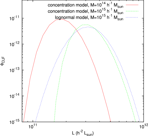
Figure 3: Examples of the calculated distribution for the BCG luminosity, for both the lognormal and concentration models, and for two different values of the halo mass.

4 Central vs satellite galaxies

As was briefly mentioned above, the way we build up the mass-luminosity relation naturally gives rise to a model for clusters, featuring a distinct separation between central and satellite galaxies. This comes from the fact that we consider that galaxies are hosted by both the parent halo and the subhaloes. Since we consider that the same mass-luminosity relation applies for both, and the former will be, by definition, considerably more massive than the latter, this results in there being a central, very luminous galaxy, hosted by the parent halo, while fainter satellite galaxies are spread throughout in the subhaloes.

Of particular importance for the question of whether the first brightest galaxies are special, this separation implies that these galaxies should indeed have a special luminosity distribution, independent from that of the remaining galaxies in the cluster. This comes from the fact that the distribution functions of these two types of galaxies will be different in origin: the central galaxies one will be determined by the halo mass function, while the satellite galaxies one will depend on the subhalo mass function. This dichotomy is also found in HOD models, for instance when accounting for total galaxy occupation number (e.g., Yang et al. 2005; Zheng et al. 2005): while $P(N|M)$, the probability that a halo of mass $M$ hosts $N$ galaxies, is Poissonian at high $N$, where satellite galaxy numbers dominate, it is significantly sub-Poissonian at low $N$, indicating that the distribution of the central galaxies is much more deterministic.

This has an important consequence, derived from the fact that, at high mass, and therefore also at high luminosity, the total mass function is dominated by the haloes, not subhaloes. This means that, when analysing the luminosity function of galaxies in clusters, the brightest region will be dominated by the central galaxies, which will actually be more abundant overall than the brightest of the satellite galaxies. We then expect that this will cause a feature in the cluster galaxy luminosity function at the bright end; this point will be examined in further detail below. Another consequence is that we expect the luminosity of the central galaxy in the cluster to be completely determined by halo mass and its distribution, without the need to account for surviving subhaloes.

It is in fact possible to derive the different contributions to the global luminosity function from the central and satellite galaxies, by associating them with the halo and subhalo distributions, respectively, and then using the CLF formalism presented in the previous section:

$$\phi_{i}(L)dL=\int_{0}^{\infty}\phi_{CLF}(L|M)n_{i}(M)dM\,,$$ (17)

where the $i$ indexes refer to the haloes and subhaloes, respectively. The derived luminosity functions for central and satellite galaxies are shown in figure 4. Unsurprisingly, the central galaxies completely dominate the overall luminosity function at high luminosity, with their numbers becoming comparable to the satellites only at low luminosity. This simply reflects the trends seen in the halo and subhalo numbers (see paper I). The expected relative contributions of both types of galaxies are still uncertain: while Benson et al. (2003a) using their semi-analytical modelling find satellite galaxies to dominate at the faint end, Cooray & Milosavljević (2005b) using a conditional luminosity function formalism find that central galaxies dominate throughout the range (likewise, Zheng et al. (2005) find that central galaxies dominate the stellar mass function on any mass scale).

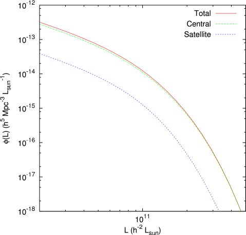
Figure 4: Contribution to the high-end luminosity function of central and satellite galaxies. These particular curves are for the $K$-band, lognormal model, but the results are similar for the concentration model. It is very noticeable that the halo numbers dominate in this luminosity range. The relative satellite contribution to the total luminosity function is qualitatively similar to what is found by other authors (van den Bosch et al., 2006).

4.1 Definition of cluster threshold mass

A necessary first step before continuing this analysis is to define precisely what we mean by a ”cluster”. We will opt for a simple choice, following the standard Abell definition of rich cluster, namely that it must have upwards of 30 objects brighter than $m_{3}+2^{m}$, where $m_{3}$ is the magnitude of the third brightest galaxy in the cluster. It is then possible, following our model, to translate this into a minimum mass threshold for a halo to host a cluster, as follows.

The third brightest galaxy will correspond to the second most massive subhalo (since the brightest galaxy is hosted by the parent halo itself), and the probability of this having a mass $m_{2}$ is then:

$$P_{2}(m_{s,2},M_{h})=N(m_{s,2}|M_{h})<N>{\rm e}^{-<N>}\,,$$ (18)

where $N(m_{s,2}|M_{h})$ is the mass distribution function of the subhaloes, equation (2), and $<N>=\int_{m_{s,2}}^{\infty}N(m^{\prime}|M_{h})dm^{\prime}$ is the average number of subhaloes more massive than $m$ in a parent halo of mass $M_{h}$. This expression assumes that the distribution of subhalo masses is Poissonian with average $<N>$, as expected for the subhaloes (e.g., Kravtsov et al. 2004; since we are looking at cluster sized haloes, $<N>$ will be large in this case), and it is simply the product of the probability of having a subhalo with mass $m_{2}$, given by the first term on the right hand side, by the Poisson probability of having exactly one subhalo more massive than $m_{2}$. Using the fact that $d<N>/dm=-N(m_{s}|M_{h})$, it is easy to check that this probability is well normalized to 1. The average value of the magnitude corresponding to this subhalo, $m_{3}$, can then be calculated from the distribution by:

$$<m_{3}(M_{h})>=\int_{0}^{\infty}m(m_{s})P_{2}(m_{s},M_{h})dm_{s}\,,$$ (19)

where $m(m_{s})$ represents the corresponding magnitude as a function of the subhalo mass, calculated using the mass-luminosity relation from section 2. In this instance, we have used the simpler relation of equation (5), since it greatly simplifies the calculations and using the full CLF results in only a slight difference.

Using this magnitude we can then obtain $m_{3}+2^{m}$, and then convert this back into a mass threshold, $m_{t}(M_{h})$, which will be dependent on the parent halo mass. Finally, we can find the probability, as a function of $M_{h}$, that $N(m_{t}|M_{h})\geq 29$ (giving more than 30 objects above the magnitude limit, when including the central galaxy). Since we are assuming that the subhalo distribution is Poissonian, this will simply be given by $\sum_{n=29}^{\infty}P(n,\mu)$, where $P(n,\mu)$ is the normal Poisson probability with average $\mu=<N(m_{t}|M_{h})>$. This gives a smooth transition for the mass of cluster hosting haloes, shown in figure 5, starting around a halo mass of $M_{h}=10^{14}h^{-1}{\rm M_{\odot}}$, but which depends on the luminosity function considered.

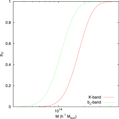
Figure 5: Probability that a halo of mass $M$ contains more than 30 galaxies brighter than $m_{3}+2^{m}$ and is considered a rich cluster according to the usual Abell definition. Using either the $b_{J}$ or the $K$ bands to do the counting results in the two different curves.

4.2 Cluster galaxy luminosity function

Once we have a mass threshold for haloes hosting clusters, obtaining the cluster galaxy luminosity function is straightforward: we simply sum up the mass function of haloes above this threshold with the mass function of all the subhaloes hosted by them (i.e., use equation (2), but further multiplied by a term to reflect the probability that the halo does indeed host a rich cluster, given by the result shown in figure 5). Then, we transform this into a luminosity function using the CLF. Our result is shown in figure 6.

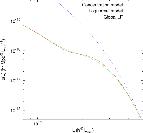
Figure 6: Luminosity function of galaxies in rich clusters, in the $K$-band. The two curves correspond to the two models for the dispersion used, described in the previous section. Also shown, for comparison, is the global LF. Only galaxies above the mass threshold shown in figure 5 were considered.

Qualitatively, we obtain a good agreement with observed luminosity functions (such as the one of de Propris et al. 2003, although in this particular case a direct comparison is difficult because these results are in a different band; redoing our analysis in the same band produces a good match), particularly in the lower luminosity range. At the bright end, there is some disagreement caused by a particular feature of our result, a bump in the luminosity function at the bright end. It is simple to understand that this bump is caused by the central galaxies. The discrepancy in numbers between central and satellite galaxies comes from the fact that, at high luminosity, the contribution from parent haloes to the total luminosity distribution (shown in figure 4) completely dominates over the subhalo one. This is a reflection of the fact that haloes are much more abundant at the high mass end than subhaloes (see paper I). In fact, it can be seen from the figure that these central galaxies essentially correspond to the high luminosity end of the global luminosity function. This is hardly surprising, since we can expect the most luminous galaxies to lie at the centre of the most massive clusters.

Such a feature is thus a natural consequence of the model: very luminous galaxies will predominantely be central galaxies of high mass haloes, which will therefore dominate in number over satellite galaxies of the same luminosity; at the same time, since we introduce a lower mass limit to rich cluster hosting haloes, the faint end contribution to the luminosity function of galaxies in such clusters will come entirely from satellites. It is important to note that this is not a particularity of this specific model: any model associating central galaxies with parent haloes and satellite galaxies with subhaloes will show a similar feature, due to the discrepancy in numbers between the two at high mass (though it may also require that this be associated with high luminosity in both cases; or, more particularly, that the same mass-luminosity relation is used for both haloes and subhaloes, as is the case in the model used here).

A note of caution comes from the fact that the shape of the bump depends on the dispersion in the CLF: the smaller it is, the sharper the bump will be. Furthermore, the actual shape of the bump is determined by the cluster definition being used, through the cluster threshold mass discussed in the previous section. This cutoff mass is responsible for the decreasing values of the cluster galaxy luminosity function on the left side of the bump; a lower threshold mass would result in a wider bump. Taking this threshold to lower and lower values (beyond the range where it would be reasonable to assume the presence of clusters) results in the progressive disappearance of the bump as we naturally regain the overall global luminosity function. It should be stressed, however, that the presence of a bump is a fundamental prediction of the model, independent of the precise cluster definition being used, since it is a direct consequence of the discrepancy in numbers between haloes and subhaloes at high mass.

This kind of feature is also present in some recent work dealing with HOD models and the central/satellite galaxy separation. In Zheng et al. (2005) (see also Zhu et al. 2006), the authors use a semi-analytical model of galaxy formation to obtain the conditional galaxy baryonic mass function. For high mass haloes in the range we are considering here, they also obtain a high mass bump in this function caused by the central galaxy. They show that the baryonic mass function can be described by combining a Schechter function representing the satellite galaxies contribution with a high mass gaussian due to the central galaxy. Likewise, Zehavi et al. (2005) build up HOD models from SDSS results, and analyze the central/satellite galaxy split; from this, they build conditional luminosity functions, and show that their results imply that the central galaxies lie far above a Schechter function extrapolation of the satellite population. The observational work also hints at similar features: for example, it is known that cD galaxies are brighter than what is given by the bright end of the cluster galaxy luminosity function (e.g., Binggeli, Sandage & Tammann 1988). This is also present in studies of the luminosity function of galaxies in clusters (e.g., Eke et al. 2004). All this once again reinforces the notion that central galaxies form a special distribution, essentially separate from the satellite galaxy one.

5 Building the BCG luminosity distribution

As discussed above, the non-parametric model used naturally builds a picture of galaxy clusters. This translates itself into a procedure to build up the total luminosity distribution of galaxies within a halo of a given mass. This will be composed of two steps, one dealing with the satellite galaxies in the subhaloes, another with the central galaxy.

5.1 Satellites

In this step, we need to sum up the total luminosity in the satellite galaxies contained in the halo. We start by taking the total number of subhaloes in a given halo, as calculated from the SHMF (that is, the occupation number; see paper I) , as an average number for a parent halo of this mass, taking into account the effect of destroyed subhaloes as introduced in section 2.1. In this step it is necessary to specify a minimum mass: we take a low enough value to ensure that we account for all subhaloes massive enough to give a noticeable contribution to the total luminosity of the halo. We then assume that the total number of subhaloes follows a Poisson distribution (as discussed above; e.g., Kravtsov et al. 2004).

For each subhalo, up to a total as calculated from the Poisson distribution, we determine a mass, by assuming the subhaloes follow a random distribution given by the subhalo mass function (2). Then we convert this to the luminosity of the hosted galaxy using the mass luminosity relation.

Finally, once we have the total number of subhaloes (as determined initially from the Poisson distribution), we can sum all of their calculated luminosities to obtain the total in satellite galaxies.

At the same time, the average luminosity of the brightest satellite galaxy can be calculated in a more direct fashion. Using the subhalo mass distribution, we can get the probability distribution of the mass of the most massive subhalo. Analogously to what was done in the previous section for the second most massive subhalo (see equation 18), this will be given by

$$P_{1}(m_{1},M_{h})=N(m_{1}|M_{h}){\rm e}^{-<N>}\,,$$ (20)

where $<N>=\int_{m}^{\infty}N(m^{\prime}|M_{h})dm^{\prime}$ as before. Used together with the mass luminosity relation, the average luminosity of the galaxy hosted in the most massive subhalo (and therefore the most luminous of the satellites) is simply given by $<L_{1}>(M_{h})=\int_{0}^{\infty}L(m_{1})P_{1}(m_{1},M_{h})dm_{1}$.

5.2 Central galaxy

The way we have built up the CLF gives us a natural way of obtaining the distribution of the luminosity of first brightest galaxies with cluster luminosity, since we are already introducing a distribution with mass. We use the results of both the lognormal and concentration models for comparison.

The total luminosity is obtained by summing over the BCG and satellite contributions, and taking into account the effect of the destroyed subhaloes from section 2.1. The average total luminosity at any given mass is simply the sum of the average luminosities of the BCG and satellites, and is, by construction, equal to the one shown in figure 2.

Finally, we can also obtain the global distribution of BCG luminosity over all clusters. To do this, we use the cluster threshold mass, as calculated in the previous section, and simply integrate the conditional distribution we have multiplied by the halo mass function:

$$f(L_{1})=\int_{0}^{\infty}f(L_{1}|M)n(M)p(M)dM\,,$$ (21)

where $n(M)$ is the halo mass function, given by (1), and $p(M)$ is the probability that a halo of mass $M$ hosts a rich cluster, as given in figure 5.

6 Other models for BCGs

In this section, we introduce two other simple models to complement the one presented above in order to allow better comparisons with the observational results. The first, and, a priori, best motivated is based on the simple assumption that the BCGs are merely the extreme values of the unique distribution that applies to all cluster galaxies. We do this based on a regular cluster galaxy luminosity function, and build the BCG distribution directly from it. The second is based on assuming some form of cannibalism. We use a simple approach to model this mechanism, that of merging the brightest galaxy with one other, where both are taken from the universal distribution in the first case we consider.

6.1 Extremes of a general distribution

The simplest assumption possible when studying the distribution of the galaxies in a cluster is that they are all drawn from the same statistical distribution (for example, a Schechter function for luminosity). The galaxies in a cluster would then simply be a random sample drawn from this distribution, with the brightest galaxy simply the extreme value of this sample. This approach has been studied in the literature before (e.g., Tremaine & Richstone 1977). In particular, it has been shown that this approach leads to a result from extreme value theory, the Gumbel distribution, for the overall distribution of the magnitudes of the first brightest galaxy (Bhavsar & Barrow, 1985; Bernstein & Bhavsar, 2000). This is given by

$$f(M)=ae^{a(M-M^{*})-e^{a(M-M^{*})}}\,,$$ (22)

with $M^{*}=M_{G}+\frac{0.577}{a}$, where $M_{G}$ is the mean of the magnitude values and $a$ is a measure of the steepness of fall of the parent distribution.

In the present paper, we take a slightly different approach, in order to match that which we will take for the other models. This model and subsquent calculations are similar to the ones presented in Tremaine & Richstone (1977), although some details, like the luminosity function used, will be different. We begin by assuming that the parent distribution of the luminosity of the galaxies in a cluster is given by a Schechter function, equation (3) (for simplicity, we use the same values for $M_{*}$ and the faint end slope, $\alpha$, as the global luminosity function).

The only dependence on the actual cluster considered comes in the normalization, which we set so that the total luminosity in all the galaxies equals the cluster luminosity, $L_{c}$:

$$\phi_{*}(L_{c})=\frac{L_{c}}{\Gamma[2-\alpha]L_{*}}\,.$$ (23)

We then take the value of the distribution of the first brightest galaxy at a given luminosity to be the probability that there are no galaxies brighter than that luminosity, times the probability that there is a galaxy at that luminosity. The latter is simply given by (3), while for the former we take a Poisson fluctuation around the average number of galaxies obtained by integrating the parent distribution, (3). Thus, the luminosity distribution for the brightest cluster galaxy is given by:

$$f_{1}(L,L_{c})=\phi(L,L_{c})e^{-\int_{L}^{\infty}\phi(L,L_{c})dL}\,,$$ (24)

where the integral in the exponential can be resolved to $\int_{L}^{\infty}\phi(L)dL=\phi_{*}(L_{c})\Gamma[1-\alpha,L/L_{*}]$. Using the same principles as discussed in section 4.1 above, it is simple to show that this probability distribution is adequately normalized to 1.

Similarly, the probability for the luminosity of the second brightest galaxy is given by the product of the probability of having a galaxy at a given luminosity by the probability of there being a single galaxy brighter than that luminosity. In general, and again taking Poisson fluctuations around the average number, the distribution of the n-th brightest galaxy will be given by:

$$f_{n}(L,L_{c})=\phi(L,L_{c})\big{(}\int_{L}^{\infty}\phi(L^{\prime})dL^{\prime}\big{)}^{n}e^{-\int_{L}^{\infty}\phi(L^{\prime})dL^{\prime}}/n!\,.$$ (25)

Likewise, the joint probability of having the first brightest galaxy at luminosity $L_{1}$ and the second at $L_{2}$ (given by the product of the probability of a galaxy at $L_{2}$, another at $L_{1}$, none in between and none above $L_{1}$) can also be derived:

$$f_{12}(L_{1},L_{2},L_{c})=\phi(L_{1},L_{c})\phi(L_{2},L_{c})e^{-\int_{L_{2}}^{\infty}\phi(L)dL}\,.$$ (26)

Once we have these distributions, it is then easy to obtain the various statistics we are interested in: the average magnitude of the first and second brightest galaxies, $<m_{1}>$ and $<m_{2}>$, the dispersion in first brightest galaxy magnitude, $\sigma_{1}$, and the average magnitude difference between these two $<\Delta_{12}>=<m_{1}-m_{2}>$. Some caution is necessary with the last one, since the fact that $L_{1}$ and $L_{2}$ are not independent variables would necessitate the use of the joint distribution; however, it turns out that the integrals over this joint distribution resolve to two different integrals over the two separate distributions, so that $<\Delta_{12}>=<m_{1}>-<m_{2}>$ as calculated for each separate, individual distribution.

6.2 Cannibalism

To illustrate the effect of galactic cannibalism, we consider here two simple models, starting with a common distribution like the one discussed in the previous section, and then merging the brightest galaxy with one of the others.

In general, the distribution of the new BCG will have to be taken from the joint distribution of the previous first and n-th brightest galaxies. It is important to note that these variables are not independent, and as such when calculating the average of the sum it will not, in principle, be possible to separate it into integrals over the two individual distributions (except in the particular case when $n=2$, as noted above).

6.2.1 $L_{1}+L_{2}$

The simplest possible model to consider when taking account of cannibalism is to merge the two brightest galaxies from a common distribution. Thus, the luminosity of the brightest galaxy is now given by the sum of the luminoisities of the previous two brightest galaxies, with a distribution given by the joint distribution of equation (26). The second brightest galaxy is now the old third brightest, with a distribution given by equation (25), with $n=3$.

The remaining calculations follow the same pattern as discussed in the previous case. It is to be expected that, due to the fact that the new first brightest luminosity is the result of the sum of two previous variables, the dispersion in first brightest luminosity will be slightly lower than before. Likewise, it is obvious that the difference in magnitude between first and second brightest galaxies will now be much larger.

6.2.2 $L_{1}+L_{n}$

A slightly more realistic toy model to illustrate galactic cannibalism is to proceed similarly as described above, but instead of merging the first brightest galaxy with the second, to take some weighting function to reflect the probability that the merger will occur with any one other of the galaxies in the cluster.

We take the probability of the merger occuring with the n-th brightest galaxy to be proportional to its average luminosity, $L_{n}$; this gives greater weight to the first few brightest galaxies, but since the average luminosity decreases only slowly with $n$, the probability is split over a wide range. We consider a possible merger down to the 30th brightest galaxy in the cluster, for which the merger probability given by this prescription will be below 1%.

The total probability distribution of the new BCG luminosity is obtained from the joint probability distribution of the different weighted pairs. Since the variables are not independent and therefore this joint distribution cannot be split into a product of terms each dependent only on a single variable, to calculate $<m_{1}>$, $<m_{2}>$ and $\sigma_{1}$ it is necessary to solve complicated integrations. We turn instead to a Monte Carlo method, building up the distribution of the new BCG luminosity by randomly generating merger pairs and the luminosity of their components, and then summing them. The new second brightest galaxy will be either the old one, or the old third brightest, depending on whether the merger occurred with the former or not.

7 Results

We start by showing the results for average magnitude of first and second brightest galaxies as a function of total cluster luminosity, for each of the models, in figures 7 and 8. The first noticeable thing is that the curves for both the concentration and lognormal models are very similar, which is not too surprising given the similar mass-luminosity relations obtained for each of them (see table 2), even though they were built in independent ways. This is in fact a success for the concentration model, since the lognormal model is by construction made to provide the best fit to the observed BCG magnitude, while the concentration model is not.

Comparing the different sets of curves, it is easy to see the differences between the models. The statistical distribution has the lowest average BCG luminosity, which is considerably higher for the other models. This comes from the fact that all other models take the BCG distribution to be special, like an additional distribution added on to the base Schechter distribution of the satellite galaxies. Looking at the average magnitude of the second brightest galaxy, the most obvious factor is that the one from the more extreme cannibalism model is much lower than the others; once again, this is unsurprising since this is essentially the third brightest galaxy in the statistical model. Likewise, the 1+n cannibalism model gives essentially the same result as the statistical one, since the second brightest galaxy is the same in both in most cases. Both of our models give considerably brighter values for the second brightest galaxy. This probably indicates that the luminosity function we used to generate the statistical and cannibalism models does not have enough bright galaxies (i.e., $L_{*}$ is too low), which is not very surprising since we are using the parameters of the global one. On the other hand, if this were to be the case then it is quite probable that the cannibalism models would then give BCGs which are too bright.

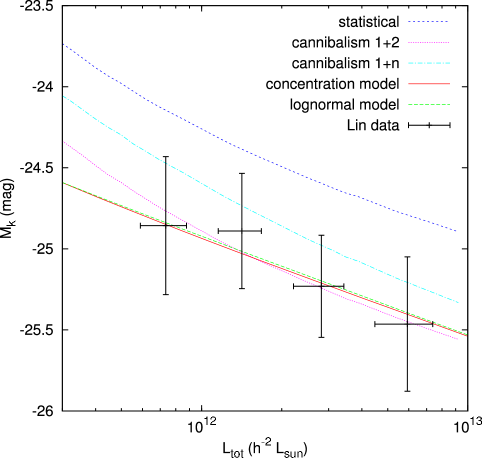
Figure 7: Average magnitudes, in the $K$-band, of the first brightest galaxy, as a function of the total cluster luminosity, as calculated for the different models: the ones based on the CLF formalism introduced, the statistical model and two forms of cannibalism: the extreme $L_{1}+L_{2}$, and the softer $L_{1}+L_{n}$. The data points shown are binned values of cluster galaxy data supplied by Yen-Ting Lin (2006, private communication).

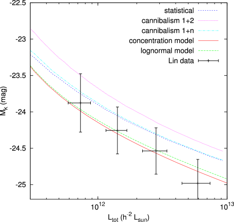
Figure 8: Same as figure 7, but for the second brightest galaxy in the cluster.

In any case, this problem should be less of an issue when looking at the magnitude gap $\Delta_{12}$, shown in figure 9. The values for the cannibalism 1+2 model are obviously much too high to match the observed ones: it is clear that merging the two brightest galaxies leaves too big a gap to the next brightest. The values for the statistical model are too low, in this case probably indicating that it is the BCG which is too faint. The values for the other, 1+n, cannibalism model look rather better, while both of our models show good agreement with the observations. But note the size of the errorbars in the observational data: the scatter in the observed values is quite large (see also Loh & Strauss 2006; van den Bosch et al. 2006). Since the scatter in the BCG magnitude is small, most of the scatter here in $\Delta_{12}$ is likely coming from the second brightest galaxy. The shape seen in the curves of figure 9 is unsurprising: the fact that $\Delta_{12}$ is increasing as the total luminosity goes down is a natural consequence of the decreasing number of satellites at this lower end. In fact, these correspond to haloes of only a few times $10^{13}h^{-1}{\rm M_{\odot}}$, and therefore many of these systems will not actually even be clusters (cf figure 5).

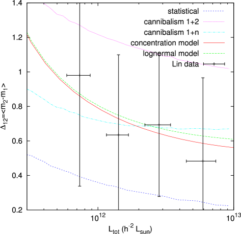
Figure 9: Values for the average magnitude difference between first and second brightest galaxies, $\Delta_{12}$. The data points come are again binned values from the catalogue supplied by Yen-Ting Lin. The large errorbars reflect the fact that the scatter in the values of $\Delta_{12}$ in these clusters is very large. For comparison, another observational value for $\Delta_{12}$, but in the $B$-band, is of $\approx 0.55$ magnitudes (Schneider, Gunn, & Hoessel, 1983). The values we obtain are also qualitatively consistent with the results of Milosavljević et al. (2006); Loh & Strauss (2006).

Figure 10 shows the calculated dispersion in the magnitude of the first brightest galaxy. Binning the Lin observational data results in values of $\sigma_{1}$ of 0.3 to 0.4 magnitudes. A direct comparison of this value with the model results shows that the values we obtain for our model are slightly too low, while the values for the statistical and cannibalism models look reasonable. There is, however, an additional point to bear in mind: these observational values are obtained by binning over a certain cluster luminosity range. Part of this observed scatter then simply comes from the fact that the average magnitude is changing as a function of this. When taking this into account, the values we get from our model are in fact in good agreement with the observed ones. Also, using Bayes’ theorem, it is possible to derive values for the dispersion in the mass of the hosting halo for a given galaxy luminosity. Doing so we obtain values which are in qualitative agreement with the ones found by van den Bosch et al. (2006), although a direct comparison is complicated by the fact that they use $b_{J}$-band instead of $K$-band for the galaxy luminosity.

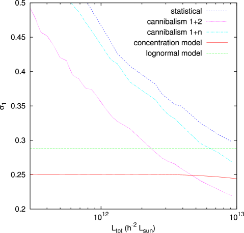
Figure 10: Dispersion in the magnitude of the first brightest galaxy. The data set used to plot the data points in the previous figures gives a value of between 0.3 and 0.4 magnitudes for the statistical error in each cluster luminosity bin. Another observationally measured dispersion in first brightest magnitude, in the $B$-band, is $\sigma_{1}\simeq 0.24$ (Postman & Lauer, 1995). Using a CLF approach similar to ours, Cooray (2006) obtains a value of $\sigma_{1}=0.17$ in the r-band.

8 Conclusion

In the present paper we focus on the implications of the mass luminosity relation first introduced in paper I on the properties of clusters, and more in particular on whether BCGs are statistical or special in nature. We expand the model of paper I by introducing scatter into the relation, building a CLF based on two different models: a simple lognormal shape or a model based on the distribution of concentrations in haloes of a given mass. We also introduce a simple model to evaluate the mass fraction in subhaloes which have been completely disrupted since they were accreted.

We have argued that this model naturally gives a separation between central and satellite galaxies in a cluster, with the former having a distinct distribution based on the halo mass function. We have shown that this leads to a characteristic bump in the cluster galaxy luminosity function, qualitatively similar to that seen in some observational work and some semi-analytical HOD based models. This is caused by the fact that, at any given high mass, haloes are considerably more abundant than subhaloes, coupled with the fact that, in any single system, central galaxies will be considerably brighter than the satellites (since the subhaloes are much less massive than the parent halo). Together with this, the faint end is completely determined by the satellite galaxies in the subhaloes, since we put in a minimum mass threshold for the haloes we consider host clusters.

Finally, to look at the question of the nature of BCGs, we study some statistical indicators that may provide a clue to this problem, namely the ratio $r$ between the magnitude difference between first and second brightest galaxies in a cluster, $\Delta_{12}$, and the dispersion of the former, $\sigma_{1}$. We also introduce two simple models to account for two different possibilities that are usually considered: the statistical hypothesis, that is, that all galaxies in a cluster, including the BCG, are drawn from the same distribution; and galactic cannibalism, where the BCG grows by merging with other galaxies in the cluster. As is already known, any model of the former gives a value for $r$ which is too small compared to what is observed. At the same time, we show that the simplest case of the latter, that of merging the two brightest galaxies from a common distribution, gives a value of $\Delta_{12}$ which is far too large.

From the results we obtain, it is possible to draw some answers to the issue discussed in the introduction about the nature of BCGs. The statistical hypothesis, which assumes that BCGs are drawn from the same universal distribution, can be ruled out. It gives values of $\sigma_{1}$ which are too big and $\Delta_{12}$ which are too small.

On the other hand, the simplistic model we analyse for galactic cannibalism looks to be far too extreme. Mainly, it gives values of $\Delta_{12}$ which are far too large compared to what is observed. This model mimics the scenario of two similar sized clusters merging, with a final distribution of galaxies which can be well fit by a single distribution, but where the BCG is then built up by merging the two BCGs of the original clusters. From our results, we expect that if such a scenario does occur, a merging of the brightest galaxies is excluded, as it leaves a too bright BCG and too large a gap to the second brightest galaxy (but see the discussion in Lin & Mohr 2004). A more general cannibalistic scenario, where the BCG is built up by merging with one other galaxy, is however not excluded, nor is the possibility of minor mergers, where one of the merging systems is much smaller than the other such that its brightest galaxy will not be the second brightest galaxy in the resulting cluster. It is worth noting that this fits in well with the results of recent semi-analytic simulations done by de Lucia & Blaizot (2006), who find that BCG growth occurs fast enough that major mergers are relatively rare, and that most of the later growth is through minor mergers.

Our model gives results which can be regarded as halfway between the other two: the BCG is in fact the product of a special distribution and is considerably brighter than what would result from a single distribution, but the second brightest galaxy is not as faint as in the cannibalistic scenario. The question remains, however, of what is the BCG formation scenario expected in this case. A satisfactory answer, in the framework of the way the mass luminosity relation is built, would require going back to the simulations and following the behaviour of the halo and its subhaloes.

There is an important assumption which has been implicit throughout this paper: that both the central and satellite galaxies follow the same mass luminosity relation. This may indeed appear to be contradictory with the possibility that the central galaxies are special, since it may seem to imply that they are formed through the same processes. On the other hand, the model is based on structure build up through the merger of dark matter haloes, and we assume that the satellite galaxies were formed in their own independent haloes, prior to being accreted into their present parent halo. This original halo would be the one that determines their properties, since the galaxy stops accreting gas or undergoing mergers of its own once its halo merges into the parent system and it becomes a satellite (and hence the need for some mass loss prescription). Therefore, it is to be expected that at least in some cases, they would have been a BCG in their own system themselves, and therefore it may not be unreasonable to assign them the same mass luminosity relation. Still, this leaves out the very important factor that the formation epoch may well be different, together with subsquent growth of the BCG in the parent system. At the same time, halo numbers completely dominate at high mass (and therefore it is to be expected the same is true of central galaxy numbers at high luminosity), and consequently the total average mass luminosity relation should be pretty much the same as calculated.

We should stress the fact that our concentration models gives quite good results, since unlike the lognormal model, it does not involve any fitting of parameters to BCG results. In fact, it is quite interesting that it gives values for the dispersion in BCG magnitude so close to the ones from the lognormal model, when the latter was set to the value that results in the best fit to the observed BCG magnitudes. In light of the recent discussion about the effects of additional parameters, such as environmental density, halo formation time or concentration (e.g., Wechsler et al. 2006; Berlind et al. 2006), on the clustering of halos and subsequently on the HOD, this seems to indicate that taking the halo mass as the primary determinant of the hosted galaxy luminosity, and then taking concentration as a secondary variable which determines the scatter around the average value is a good way to proceed.

References

- Benson et al. (2003a) Benson A. J., Frenk C. S., Baugh C. M., Cole S., Lacey C. G., 2003, MNRAS, 343, 679
- Bhavsar (1989) Bhavsar S.P., 1989, ApJ, 338, 718
- Bhavsar & Barrow (1985) Bhavsar S.P., Barrow J.D., 1985, MNRAS, 213, 857
- Berlind & Weinberg (2002) Berlind A. A., Weinberg D. H., 2002, ApJ, 575,587
- Berlind et al. (2006) Berlind A.A., Kazin E., Blanton M.R., Pueblas S., Scoccimarro R., Hogg D.W., astro-ph/0610524, submitted to ApJ
- Bernardi et al. (2006) Bernardi M., Hyde J.B., Sheth R.K., Miller C.J., Nichol R.C., 2006, ApJ, in press, astro-ph/0607117
- Bernstein & Bhavsar (2000) Bernstein J.P., Bhavsar S.P., 2000, MNRAS
- Binggeli, Sandage & Tammann (1988) Binggeli B., Sandage A., Tammann G.A., 1988, ARA&A, 26, 509
- Bullock et al. (2001) Bullock, J. S., Kolatt, T. S., Sigad, Y., Somerville, R. S., Kravtsov, A. V., Klypin, A. A., Primack, J. R., Dekel, A., 2001, MNRAS, 321, 559
- Capaccioli (1989) Capaccioli M., 1989, in The World of Galaxies, ed. H.G. Corwin& L. Bottinelli, Springer, Berlin, 208
- Colless (1989) Colless M., 1989, MNRAS, 237, 799
- Conroy, Wechsler & Kravtsov (2006) Conroy C., Wechsler R.H., Kravtsov A.V., 2006, ApJ, 647, 201
- Cooray (2006) Cooray A., 2006, MNRAS, 365, 842
- Cooray & Milosavljević (2005a) Cooray A., Milosavljević M., 2005a, ApJ, 627, L85
- Cooray & Milosavljević (2005b) Cooray A., Milosavljević M., 2005b, ApJ, 627, L89
- de Lucia & Blaizot (2006) De Lucia G., Blaizot J., 2006, MNRAS, accepted, astro-ph/0606519
- de Propris et al. (2003) De Propris R. et al., 2003, MNRAS, 342, 725
- Dressler (1978) Dressler A., 1978, ApJ, 222, 23
- Eke et al. (2004) Eke V.R. et al., 2004, MNRAS, 355, 769
- Gao et al. (2004) Gao L., White S.D.M., Jenkins A., Stoehr F., Springel V., MNRAS, 355, 819
- Graham et al. (1996) Graham A., Lauer T.R., Colless M., Postman M., 1996, ApJ, 465, 534
- Hausman & Ostriker (1978) Hausman M.A., Ostriker J.P., 1978, ApJ, 224, 320
- Hoessel, Gunn & Thuan (1980) Hoessel J.G., Gunn J.E., Thuan T.X., 1980, ApJ, 241, 486
- Hoessel & Schneider (1985) Hoessel J.G., Schneider D.P., 1985, AJ, 90, 1648
- Kochanek et al. (2001) Kochanek C. S., et al., 2001, ApJ, 560, 566
- Kravtsov et al. (2004) Kravtsov A. V., Berlind A. A., Wechsler R. H., Klypin A. A., Gottlöber A., Allgood B., Primack J. R., 2004, ApJ, 609, 35
- Lin & Mohr (2004) Lin Y., Mohr J.J., 2004, ApJ, 617, 879
- Lin, Mohr & Stanford (2004) Lin Y., Mohr J.J., Stanford S.A., 2004, ApJ, 610, 745
- von der Linden et al. (2006) von der Linden A., Best P.N., Kauffmann G., White S.D.M., 2006, astro-ph/0611196, submitted to MNRAS
- Loh & Strauss (2006) Loh Y., Strauss M.A., 2006, MNRAS, 366, 373
- Macciò et al. (2006) Macciò A.V., Dutton A.A., van den Bosch F.C., Moore B., Potter D., Stadel J., 2006, astro-ph/0608157, submitted to MNRAS
- Milosavljević et al. (2006) Milosavljević M., Miller C.J., Furlanetto S.R., Cooray A., 2006, ApJ, 637, L9
- Navarro, Frenk, & White (1997) Navarro J. F., Frenk C. S., White S. D. M., 1997, ApJ, 490, 493
- Norberg et al. (2002) Norberg P. et al., 2002, MNRAS, 336, 907
- Ostriker & Hausman (1977) Ostriker J.P., Hausman M. A., 1977, ApJ, 217, L125
- Ostriker & Tremaine (1975) Ostriker J.P., Tremaine S.D., 1975, ApJ, 202, 113
- Peebles (1968) Peebles, P.J.E., 1968, ApJ, 153, 13
- Postman & Lauer (1995) Postman M., Lauer T.R., 1995, ApJ, 440, 28
- Sandage (1972) Sandage, A., 1972, ApJ, 178, 1
- Schneider, Gunn, & Hoessel (1983) Schneider D. P., Gunn J. E., Hoessel J. G., 1983, ApJ, 268, 476
- Shaw et al. (2006) Shaw L., Weller J., Ostriker J.P., Bode P., 2006, ApJ, 646, 815
- Sheth & Tormen (1999) Sheth R. K., Tormen G., MNRAS, 1999, 308, 119
- Spergel et al. (2006) Spergel D. N. et al., 2006, astro-ph/0603449, submitted to ApJ
- Tasitsiomi et al. (2004) Tasitsiomi A., Kravtsov A. V., Wechsler R. H., Primack J. R., 2004, ApJ. 614, 533
- Tremaine & Richstone (1977) Tremaine S.D., Richstone D.O., 1977, ApJ, 212, 311
- Vale & Ostriker (2004) Vale A., Ostriker J. P., 2004, MNRAS, 353, 189
- Vale & Ostriker (2006) Vale A., Ostriker J. P., 2006, MNRAS, 371, 1173 (Paper I)
- van den Bosch, Tormen & Giocoli (2005) van den Bosch F. C., Tormen G., Giocoli C., 2005, MNRAS, 359, 1029
- van den Bosch et al. (2006) van den Bosch F.C. et al., 2006, astro-ph/0610686, submitted to MNRAS
- Wang et al. (2006) Wang L., Li C., Kauffmann G., De Lucia G., 2006, MNRAS, 371, 537
- Wechsler et al. (2006) Wechsler R.H., Zentner A.R., Bullock J.S., Kravtsov A.V., 2006, ApJ, in press, astro-ph/0512416
- Weller et al. (2005) Weller J., Ostriker J. P., Bode P., Shaw L., 2005, MNRAS, 364, 823
- Yagi et al. (2002) Yagi M., Kashikawa N., Sekiguchi M., Doi M., Yasuda N., Shimasaku K., Okamura S., 2002, AJ, 123, 87
- Yang et al. (2003) Yang X.H., Mo H.J., van den Bosch F.C., 2003, MNRAS, 339, 1057
- Yang et al. (2005) Yang X.H., Mo H.J., Jing Y.P., van den Bosch F.C., 2005, MNRAS, 358, 217
- Zehavi et al. (2005) Zehavi I. et al., 2005, ApJ, 630, 1
- Zentner et al. (2005) Zentner A.R., Berlind A.A., Bullock J.S., Kravtsov A.V., Wechsler R.H., 2005, ApJ, 624, 505
- Zheng et al. (2005) Zheng Z. et al., 2005, ApJ, 633, 791
- Zhu et al. (2006) Zhu G., Zheng Z., Lin, W.P., Jing Y.P., Kang X., Gao L., 2006, astro-ph/0601120, submitted to ApJ