Finding Binary Millisecond Pulsars with the Hough Transform

Abstract

The Hough transformation has been used successfully for more than four decades. Originally used for tracking particle traces in bubble chamber images, this work shows a novel approach turning the initial idea into a powerful tool to incoherently detect millisecond pulsars in binary orbits.

This poster presents the method used, a discussion on how to treat the time domain data from radio receivers and create the input ”image” for the Hough transformation, details about the advantages and disadvantages of this approach, and finally some results from pulsars in 47 Tucanae.

Introduction

The problem of discovering millisecond pulsars in binary orbits is apparent. Not only the parameter range for isolated pulsars has to be addressed, but — at least — five Keplerian parameters have to be included additionally. A simple Fourier analysis is not sufficient for this class of pulsars, since the signal is smeared out over a large frequency band due to Doppler’s effect (ref. Figure. 2).

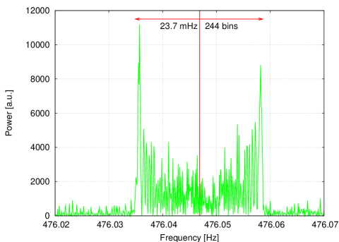
Figure 1: Power spectrum of the binary pulsar 47 Tuc J.

Over the past decades quite a few search algorithms have been devised to counter this problem, e.g. the very successful “acceleration search” [1] or the sideband search [2]. However, these approaches work purely on coherent data sets, thus they are ultimately limited by the maximum possible length of an observation

We would like to present an alternative approach to search for weak pulsars in a binary orbit, which utilizes data taken in several observation runs. In the following section we will briefly explain how the Hough transformation works, and how it can be applied to search for binary, millisecond pulsars before summarizing some of the results obtained for 47 Tucanae.

The Hough transformation

Paul Hough developed and patented the algorithm around 1960. The original algorithm was designed to search for straight particle traces in bubble chamber images by simply turning the usual line equation $y=ax+b$ into a parameter space equation $b=y-ax$.

From these two equations it is obvious that a line in the original space (“xy-space”) corresponds to a single point in the parameter space (“ab-space”). On the other hand a single point in xy-space is represented by a line in ab-space. Although sounding trivial, it actually solves a complex problem: Identifying parameters of lines found in (pixel) images.

Figure 2 shows what happens when transforming many points from a single line. For each of these points a line is drawn in ab-space and since each of these points belong to the same xy-line, their lines are required to intersect in a single point in ab-space. Naturally, random points in xy-space convert to random lines in ab-space only adding up to a random background.

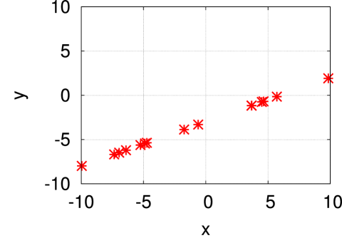
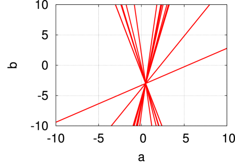
Figure 2: Points from a line in xy-space transform into lines intersecting in a single ab-point.

Tracking millions of lines along with their intersections is costly in terms of computing power and memory, thus we chose to discretize the ab-space into rectangular pixels and simply count how many lines are drawn through each pixel. This approach allows us to discover the blue “line” in Figure 3, where only 95 signal points are hidden beneath 200,000 noise points while still be detectable at an SNR of about 20!

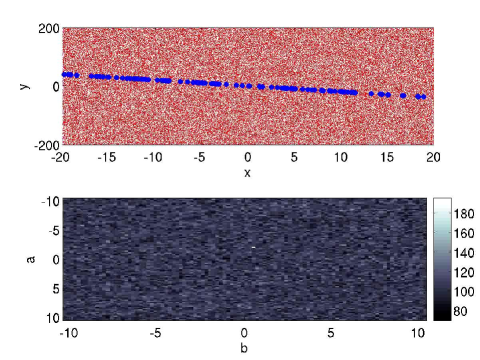
Figure 3: Recovering a hidden line (top,blue) with a SNR of about 20 (tiny white point (bottom)).

For binary pulsars, the frequency signature can be described by

$$f(t)=f_{p}(1+\lambda_{o}\cos(2\pi f_{o}-\Phi_{o})),$$

where $f_{p}$ is the intrinsic frequency of the pulsar, $f_{o}$ the orbital frequency, $\lambda_{o}$ the (dimensionless) frequency amplitude due to Doppler modulation and $\Phi_{o}$ the orbital phase at $t=0$. This equation can be recast into a line equation

$$C = Ax+By,\mbox{ where}$$

$$A = \sin(2\pi f_{o}-\Phi_{o}),$$

$$B = \cos(2\pi f_{o}-\Phi_{o}),$$

$$C = (f(t)-f_{p})/f_{p},$$

$$x = f_{p}\lambda_{o}\sin\Phi_{o},$$

$$y = f_{p}\lambda_{o}\cos\Phi_{o}.$$

Here, we split the variables into two types:

$\lambda_{o}$, $\Phi_{o}$:

These variables are considered in the Hough transform, i.e. the resulting Hough planes (formerly ab-space) are polar diagrams in these parameters.

$f_{p}$, $f_{o}$:

Called “external” variables, because they appear only as input parameters to the Hough transform and are varied outside the scope of it. This separation allows us to distribute the work onto a cluster of computers.

So far, we have not said anything about our “input image”. From the time domain data we use small pieces of the data (typically a few minutes), create a power spectrum for each piece and select peaks from the spectra. Then, we draw the registered peaks into a time-frequency plane which serves as our input for the Hough transformation.

47 Tucanae results

In this section we summarize some results obtained from 47 Tucanae data. Figure 4 shows the outcome obtained for the full parameter space ($f_{p}$, $P_{o}=f_{o}^{-1}$).

The maximum number counts (of how many lines are drawn through any pixel) found in each of the about $10^{9}$ computed Hough planes are color coded in this image. One can clearly see the signatures of several noise sources (lines at and below 100 Hz as well as pulsars (173 Hz, 186 Hz) and their harmonics at twice, thrice, … of the fundamental frequency.

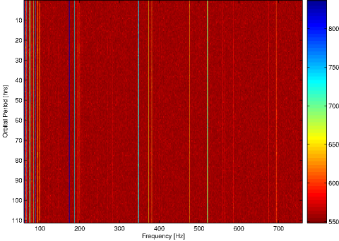
Figure 4: 47 Tucanae global result map

A closer look at the Hough planes reveals that 47 Tucanae C at 173.709 Hz is an isolated pulsar (Figure 5). Please recall that such a source does not feature any noticeable Doppler modulation in the solar system barycenter and the parameter $\lambda_{o}$ is therefore equal to zero. This in turn is shown by the maximum at the center/origin.

For the binary pulsar 47 Tucanae J the situation is different. It orbits its companion in less than 3 hours and the maximal measurable Doppler shift for this system is about 12 mHz. Figure 6 shows the Hough plane featuring the maximum at a distance to the origin corresponding exactly to this Doppler shift.

More already known pulsars have been found in the data set, but are not displayed here, please refer to [3] for more information.

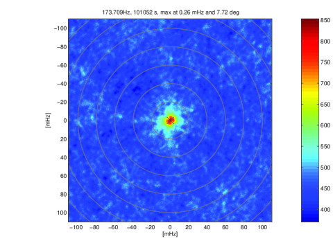
Figure 5: 47 Tucanae C: The maximum in this Hough plane is at the origin, suggesting no Doppler modulation of the signal (isolated pulsar).

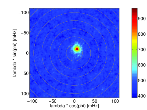
Figure 6: 47 Tucanae J: The maximum in this Hough plane is not at the origin anymore. The offset indicates a Doppler modulation of about 12 mHz agreeing well with literature values.

Summary

Although this new method has not revealed any new pulsars in the well observer globular cluster 47 Tucanae (yet), many already known pulsars have been “rediscovered” in a blind search. Since the obtained parameters for these sources agree remarkably well with the already published values, the method has proven to be principally able to discover new pulsars.

The most important advantage over “classical” search algorithms is the semi-coherent approach, allowing to combine data taken on several occasions into a single, more sensitive search. However, it should be noted that the Hough transform requires a large amount of CPU power, a typical search over a frequency bandwidth of a few hundred Hz can easily take several 10,000 CPU-hours — the current focus is to lower this number.

Finally, the author would like to thank the pulsar group at the Jodrell Bank observatory, especially Michael Kramer and Dunc Lorimer, and the Albert-Einstein-Institute for the opportunity to work on this project over the past years. At AEI especially the members of the data analysis group proved to be invaluable sources of knowledge. Special thanks go to Maria Alessandra Papa, Curt Cutler, Bernard Schutz, Alicia Sintes, Steffen Grunewald, Bernd Machenschalk, Badri Krishnan, Reinhard Prix and many more!

References

- [1] John Middleditch and Jerome Kristian. A search for young, luminous optical pulsars in extragalactic supernova remnants. Astrophysical Journal, 279:157–161, April 1984.
- [2] S. M. Ransom, J. M. Cordes, and S. S. Eikenberry. A New Search Technique for Short Orbital Period Binary Pulsars. Astrophysical Journal, 589:911–920, June 2003.
- [3] Carsten Aulbert. Finding Millisecond Binary Pulsars in 47 Tucanae by Applying the Hough Transformation to Radio Data. PhD thesis, Albert Einstein Institute, Potsdam, Germany, 2006.
- [4] Alicia M. Sintes and Badri Krishnan. Improved hough search for gravitational wave pulsars. Journal of Physics Conference Series, 32:206, 2006.
- [5] Badri Krishnan. Wide parameter search for isolated pulsars using the hough transform. Classical and Quantum Gravity, 22:S1265, 2005.
- [6] Badri Krishnan, Alicia M. Sintes, M. A. Papa, Bernard F. Schutz, Sergio Frasca, and Cristiano Palomba. The hough transform search for continuous gravitational waves. Physical Review D, 70:082001, 2004.