Hemispherical power asymmetry in the three-year
Wilkinson Microwave Anisotropy Probe sky maps

Abstract

We consider the issue of hemispherical power asymmetry in the three-year WMAP data, adopting a previously introduced modulation framework. Computing both frequentist probabilities and Bayesian evidences, we find that the model consisiting of an isotropic CMB sky modulated by a dipole field, gives a substantially better fit to the observations than the purely isotropic model, even when accounting for the larger prior volume. For the ILC map, the Bayesian log-evidence difference is $\sim 1.8$ in favour of the modulated model, and the raw improvement in maximum log-likelihood is 6.1. The best-fit modulation dipole axis points toward $(l,b)=(225^{\circ},-27^{\circ})$, and the modulation amplitude is 0.114, in excellent agreement with the results from the first-year analyses. The frequentist probability of obtaining such a high modulation amplitude in an isotropic universe is $\sim 1$%. These results are not sensitive to data set or sky cut. Thus, the statistical evidence for a power asymmetry anomaly is both substantial and robust, although not decisive, for the currently available data. Increased sky coverage through better foreground handling and full-sky and high-sensitivity polarization maps may shed further light on this issue.

1. Introduction

While the first-year results from the Wilkinson Microwave Anisotropy Probe (WMAP) experiment (Bennett et al., 2003) overall clearly supported the currently popular inflationary cosmological model, describing a flat, isotropic and homogeneous universe seeded by Gaussian and adiabatic fluctuations, a disturbing number of unexpected anomalies on large scales were reported shortly after the public data release. Perhaps the three most important ones were: 1) alignments and symmetry features among low $\ell$ multipoles (de Oliveira-Costa et al., 2004; Eriksen et al., 2004a), 2) an apparent asymmetry in the distribution of fluctuation power in two opposing hemispheres (Eriksen et al., 2004b; Hansen et al., 2004), and 3) a peculiar cold spot in the southern hemisphere (Vielva et al., 2004; Cruz et al., 2005). All of these features were subsequently studied extensively by independent groups, and all remain unresolved to the present day.

In March 2006 the three-year WMAP results were released, prompting researchers to revisit the anomalies detected in the first-year data (Bridges et al., 2006; Copi et al., 2006; Jaffe et al., 2006; Land & Magueijo, 2006; Martínez-González et al., 2006). Of course, considering that already the first-year data were strongly signal-dominated on the scales of interest, it should come as no surprise that most of these analyses concluded with similar results as for the previous data, although different foreground handling could affect some results.

The WMAP team paid particular attention to the question of large-scale power asymmetry in their analyses (Hinshaw et al., 2007; Spergel et al., 2007a). Specifically, in an early version of their paper, Spergel et al. (2007a) approached the problem from a semi-Bayesian point of view, by defining a parametric model consisting of an isotropic and Gaussian CMB field modulated by a large-scale function. The power asymmetry anomaly was then addressed by a dipolar modulation field, and the low-$\ell$ alignment anomalies were studied with a quadrupole modulation field. However, due to several issues with this early analysis, several of which were first addressed by the present paper, the authors decided to remove the corresponding section from the final version of their paper (Spergel et al., 2007b). One example is simple marginalization over non-cosmological monopoles and dipoles components, which was first done by Gordon (2007) in an otherwise identical analysis. A second example was the limited harmonic range considered by Spergel et al. (2007a). Thus, we present in this Letter the first complete modulation analysis that covers the full range of angular scales presented by Eriksen et al. (2004b), and that takes into account all known sources of systematics, such as monopole/dipole and foreground marginalization. We also present the first proper computation of the Bayesian evidence for the modulated model.

Following the first report of the power asymmetry, much effort has been spent by theorists on providing possible physical explanations. Examples range from those questioning the very fundamentals of physics and cosmology (e.g., introducing intrinsically inhomogeneous cosmologies – Moffat 2005 and Jaffe et al. 2005; violation of Lorenz invariance – Kanno & Soda 2006; or violation of rotational invariance in the very early universe – Ackermann, Carroll & Wise 2007) to those essentially considering special cases of established physics (e.g., second-order gravitational effects from local inhomogeneities – Tomita 2005; the presence of local voids – Inoue & Silk 2006; spontaneous isotropy breaking from non-linear response to long-wavelength density fluctuations – Gordon et al. 2005).

2. Algorithms

We now outline the methods used for the analyses presented in the following sections.

2.1. Data model and likelihood

We model the CMB temperature sky maps as

$$\mathbf{d}(\hat{\mathbf{n}})=\mathbf{s}(\hat{\mathbf{n}})[1+f(\hat{\mathbf{n}})]+\mathbf{n}(\hat{\mathbf{n}}),$$ (1)

where $\mathbf{s}(\hat{\mathbf{n}})$ is a statistically isotropic and Gaussian random field with power spectrum $C_{\ell}$, $f(\hat{\mathbf{n}})$ is a dipole modulation field with amplitude less than unity, and $\mathbf{n}(\hat{\mathbf{n}})$ is instrumental noise. Thus, the modulated signal component is an anisotropic, but still Gaussian, random field, and therefore has a covariance matrix given by

$$\tilde{\mathbf{S}}(\hat{\mathbf{n}},\hat{\mathbf{m}})=[1+f(\hat{\mathbf{n}})]\mathbf{S}(\hat{\mathbf{n}},\hat{\mathbf{m}})[1+f(\hat{\mathbf{m}})],$$ (2)

where

$$\mathbf{S}(\hat{\mathbf{n}},\hat{\mathbf{m}})=\frac{1}{4\pi}\sum_{\ell}(2\ell+1)C_{\ell}P_{\ell}(\hat{\mathbf{n}}\cdot\hat{\mathbf{m}}).$$ (3)

Taking into account instrumental noise and possible foreground contamination, the full covariance matrix is

$$\mathbf{C}(\hat{\mathbf{n}},\hat{\mathbf{m}})=\tilde{\mathbf{S}}(\hat{\mathbf{n}},\hat{\mathbf{m}})+\mathbf{N}+\mathbf{F}.$$ (4)

The noise and foreground covariance matrices depend on the data processing, and will be described in greater detail in §3. With these definitions ready at hand, the log-likelihood is given by

$$-2\log\mathcal{L}=\mathbf{d}^{T}\mathbf{C}^{-1}\mathbf{d}+\log|\mathbf{C}|,$$ (5)

up to an irrelevant constant.

2.2. Posterior distributions and choice of parameters

The posterior distribution $P(\theta|\mathbf{d})$ is a primary goal of any Bayesian analysis, $\theta$ being the set of all free parameters in the model. For the model defined above, the free parameters can be divided into two groups, namely those describing the isotropic CMB covariance matrix or $C_{\ell}$, and those describing the modulation field. Both may be parametrized in a number of different ways, and these choices may affect the outcome of the analysis through different prior definitions.

First, for the isotropic CMB component, we choose to parametrize the power spectrum in terms of a simple two-parameter model with free amplitude $q$ and tilt $n$,

$$C_{\ell}=q\left(\frac{\ell}{\ell_{0}}\right)^{n}C_{\ell}^{\textrm{fid}}.$$ (6)

Here $\ell_{0}$ is a pivot multipole and $C_{\ell}^{\textrm{fid}}$ is a fiducial model, in the following chosen to be the best-fit power law spectrum of Hinshaw et al. (2007). Second, the modulation field $f(\hat{n})$ is parametrized in terms of a direction $\hat{\mathbf{p}}$ and an overall amplitude $A$,

$$f(\hat{\mathbf{n}})=A\,\hat{\mathbf{n}}\cdot\hat{\mathbf{p}}.$$ (7)

We use flat priors on all parameters in this paper; the modulation axis is uniform over the sphere, and the amplitude is restricted to $A\leq 0.3$. The power spectrum parameters are restricted to $0.5\leq q\leq 1.5$ and $-0.5\leq n\leq 0.5$. These choices are sufficiently generous to include all non-zero parts of the likelihood.

The posterior distribution,

$$P(q,n,A,\hat{\mathbf{p}}|\mathbf{d})\propto\mathcal{L}(q,n,A,\hat{\mathbf{p}})P(q,n,A,\hat{\mathbf{p}}),$$ (8)

is then mapped out using a standard Markov Chain Monte Carlo technique. We use a Gaussian proposal density for $q$, $n$, and $A$, and an Euler-matrix based, uniform proposal density for $\hat{\mathbf{p}}$.

2.3. Bayesian evidence and nested sampling

In a Bayesian analysis, one is not only interested in the set of best-fit parameter values, but also in the relative probability of competing models. The most direct way of measuring this is through the Bayesian evidence,

$$E\equiv P(\mathbf{d}|H)=\int P(\mathbf{d}|\theta,H)P(\theta|H)d\theta,$$ (9)

which is simply the average likelihood over the prior volume. Typically, one computes this quantity for two competing models, $H_{0}$ and $H_{1}$, and considers the difference $\Delta\log E=\log E_{1}-\log E_{0}$. If $\Delta\log E>1$, the evidence for $H_{1}$ is considered substantial; if $\Delta\log E>2.5$, it is considered strong.

Traditionally, computation of evidences has been a computational challenge. However, Mukherjee et al. (2006) introduced a method called “nested sampling”, proposed by Skilling (2004), to the cosmological community that allows for accurate estimation of the evidence through Monte Carlo sampling. We implemented this for the priors and likelihood described above, and found that it works very well for the problem under consideration.

2.4. Maximum-likelihood analysis

We also perform a standard frequentist maximum-likelihood analysis by computing the maximum-likelihood modulation parameters for isotropic Monte Carlo simulations. For these computations, we use a modified version of the evidence code, which we find to be considerably more robust than a simple non-linear search; while the non-linear search algorithms often get trapped in local minima, the nested sampling algorithm always find the correct solution, but of course, at a considerably higher computational expense.

3. Data

We analyze two versions of the three-year WMAP sky maps in the following; the template-corrected $Q$-, $V$-, and $W$-band maps, and the “foreground cleaned” Internal Linear Combination (ILC) map (Hinshaw et al., 2007). All maps are processed as described by Eriksen et al. (2006): They are first downgraded to HEALPix resolution $N_{\textrm{side}}=16$, by additional smoothing to a $9^{\circ}$ FWHM Gaussian beam and appropriate pixel window. Second, uniform Gaussian noise of $\sigma_{\textrm{n}}=1\,\mu\textrm{K}$ is added to each pixel in order to regularize the pixel-pixel covariance matrix. This combination of smoothing and noise level results in a signal-to-noise ratio of unity at $\ell=40$, and strong noise domination at the Nyquist multipole of $\ell=47$.

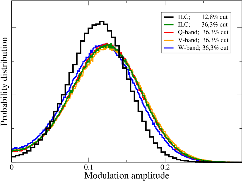
Figure 1.— Posterior distributions for the dipole modulation amplitude, marginalized over direction and CMB power spectrum.

We use two different sky cuts for our analyses. First, given that the galactic plane is clearly visible in the single frequency data, our first mask is conservatively defined. This cut is created by expanding the Kp2 mask Hinshaw et al. (2007) by $9^{\circ}$ in all directions, and then manually removing all near-galactic pixels for which any difference map between two channels are clearly larger than noise. In total, 36.3% of all pixels are rejected by this cut (see figure 2). Second, we also adopt the directly downgraded Kp2 cut used by the WMAP team that removes 12.8% of all pixels. We use this mask for the ILC map only.

The noise covariance matrix is given by the uniform noise only, $N_{ij}=\sigma_{\textrm{n}}^{2}\delta_{ij}$. For completeness, we have also computed the noise covariance from the smoothed instrumental noise for the $V$-band data, but we find that this has no effect on the final results, since its amplitude is far below the CMB signal. It is therefore omitted in the following.

Table 1

Data	($l_{\textrm{bf}},b_{\textrm{bf}}$)	$A_{\textrm{bf}}$	$\Delta\log\mathcal{L}$	$\Delta\log E$	$P$
ILC	($225^{\circ},-27^{\circ}$)	$0.114$	6.1	$1.8\pm 0.2$	0.991
ILC	($208^{\circ},-27^{\circ}$)	$0.125$	6.0	$1.8\pm 0.2$	0.991
$Q$-band	($222^{\circ},-35^{\circ}$)	$0.124$	5.5	$1.5\pm 0.2$	0.987
$V$-band	($205^{\circ},-19^{\circ}$)	$0.127$	5.6	$1.5\pm 0.2$	0.990
$W$-band	($204^{\circ},-31^{\circ}$)	$0.121$	5.2	$1.3\pm 0.2$	0.985

Note. — Modulation model results. The listed quantities are the marginal best-fit dipole axis (second column) and amplitude (third column); the change in likelihood at the posterior maximum, $\Delta\log\mathcal{L}=\log\mathcal{L}_{\textrm{mod}}-\log\mathcal{L}_{\textrm{iso}}$, between the modulated and the isotropic model (fourth column); the Bayesian evidence difference, $\Delta\log E=\log E_{\textrm{mod}}-\log E_{\textrm{iso}}$ (fifth column); and the frequentist probability for obtaining a lower maximum-likelihood modulation amplitude than the observed one, computed from isotropic simulations (sixth column).

As an additional hedge against foreground contamination, we marginalize over a set of fixed spatial templates, $\mathbf{t}_{i}$, through the covariance matrix $\mathbf{F}_{i}=\alpha_{i}\mathbf{t}_{i}\mathbf{t}_{i}^{T}$, $\alpha_{i}\gtrsim 10^{3}$. Monopole and dipole terms are always included, and one or more foreground templates. For the $V$-band and ILC maps, we follow Hinshaw et al. (2007) and adopt $V$–ILC as our foreground template. For the $Q$-band data, we marginalize over a synchrotron (Haslam et al., 1982), a free-free (Finkbeiner, 2003), and a dust (Finkbeiner et al., 1999) template individually. Finally, for the $W$-band data, we use the $W$–ILC difference map. However, we have tried various combinations for all maps, and there is virtually no sensitivity to the particular choice, or indeed, to the template at all, due to the conservative sky cut used.

4. Results

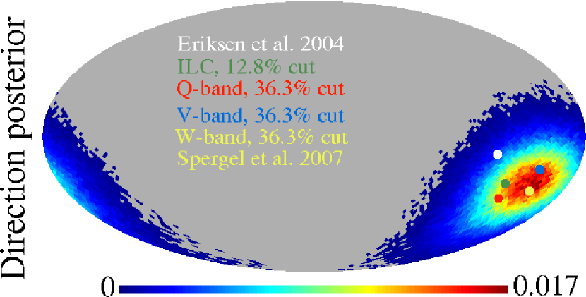
Figure 2.— Posterior distribution for the dipole modulation axis, shown for the ILC map and 36.3% sky cut, and marginalized over power spectrum and amplitude parameters. Grey sky pixels indicate pixels outside the $2\sigma$ confidence region. The dots indicate the axis 1) reported by Eriksen et al. (2004) in white; 2) for the ILC map with a 12.8% sky cut in green; 3) for the $Q$-, $V$-, and $W$-bands in red, blue and yellow, respectively. The axis reported by Spergel et al. (2007a) coincides with the $W$-band axis.

The results from the analysis outlined above are summarized in Table 1. For each map, we report the best-fit dipole axis and amplitude, as well as the maximum log-likelihood difference and Bayesian evidence difference for the modulated versus the isotropic model. The errors on the evidence are estimated by performing eight independent analyses for each case, and computing the standard deviation (Mukherjee et al., 2006). We also compute the probability of obtaining a smaller modulation amplitude than the observed one by analyzing 1000 isotropic Monte Carlo simulations.

Starting with the first case in Table 1, the ILC map cut by a 12.8% mask, we see that the best-fit modulation axis points toward $(l,b)=(225^{\circ},-27^{\circ})$, and the corresponding modulation amplitude is 0.114. The raw likelihood improvement is $\Delta\log\mathcal{L}=6.1$. The probability of finding such a high modulation amplitude in intrinsically isotropic simulations is $\sim 1$%, and, finally, the improvement in Bayesian evidence is $\Delta\log E=1.8$.

Further, these results are not sensitive to data set or sky coverage: Even the Q-band map, which presumably is the least reliable with respect to residual foregrounds, yields a modulation amplitude which is high at the 98.7% (frequentist) confidence level, and a Bayesian log-evidence improvement of 1.5. This frequency independence is further illustrated in Figure 1, where we show the marginalized posterior distributions for the modulation amplitudes for each data set. The agreement among data sets is very good.

In Figure 2 we show the dipole axis posterior distribution for the ILC map and 36.3% sky cut. Superimposed on this, we have also marked the first-year asymmetry axis reported by Eriksen et al. (2004b) [$(l,b)=(237^{\circ},-10^{\circ})$] in yellow, and also the other axes listed in Table 1. All agree well within $2\sigma$, and this is another testimony to the excellent stability of the effect with respect to statistical method, data set and overall procedure.

Finally, we note that this model may also partially explain the anomalous cold spot reported by Vielva et al. (2004) and Cruz et al. (2005): By demodulation the spot would increase its temperature by about 10%, and although still very cold, it would be significantly less extreme. Similar arguments could possibly also be made for the Bianchi VII_h correlation found by Jaffe et al. (2005). These issues will be considered further in future work.

5. Conclusions

A notable power asymmetry between two opposing hemispheres in the first-year WMAP sky maps was reported by Eriksen et al. (2004b). This feature may be observed as strong fluctuations in the southern ecliptic hemisphere, but virtually no large-scale structure in the northern ecliptic hemisphere (e.g., Hinshaw et al. 2007).

In this Letter, we have revisited this issue in the three-year WMAP data, adopting the statistical framework introduced and applied by Spergel et al. (2007a). With these tools, we find that the evidence for power asymmetry in the WMAP data is very consistent with that initially reported for the first-year maps by Eriksen et al. (2004b), and the WMAP data clearly suggest a dipolar distribution of power on the sky: The best-fit modulation amplitude is roughly 12% in real space, or about 20% in terms of power spectra. The corresponding dipole direction is $(l,b)\sim(225^{\circ},-27^{\circ})$. All results are independent of data set choices, i.e., frequency channel or sky cut.

However, the statistical evidence for this effect is still only tentative. In frequentist language, the significance is about 99%, while in Bayesian terms, the log-evidence difference is $\sim 1.5$ to 1.8, corresponding to odds of one to five or six. This is quite comparable to the evidence for $n_{\textrm{s}}\neq 1$ after the three-year WMAP data release, for which the odds are about one to eight in the highest case (Parkinson et al. 2006). Thus, there is still a chance that the effect may be a fluke, and most likely, this will remain the situation until Planck provides new data in some five years. With additional frequency coverage, a better job can be done on foreground treatment, and more sky coverage can be reliably included in the analysis. Second, full-sky and high-sensitivity polarization data should provide valuable insights on the origin of the effect.

References

- Ackerman et al. (2007) Ackerman, L., Carroll, S. M., & Wise, M. B. 2007, [astro-ph/0701357]
- Bennett et al. (2003) Bennett, C. L., et al. 2003, ApJS, 148, 1
- Bridges et al. (2006) Bridges, M., McEwen, J. D., Lasenby, A. N., & Hobson, M. P. 2006, [astro-ph/0605325]
- Copi et al. (2006) Copi, C. J., Huterer, D., Schwarz, D. J., & Starkman, G. D. 2006, [astro-ph/0605135]
- Cruz et al. (2005) Cruz, M., Martínez-González, E., Vielva, P., & Cayón, L. 2005, MNRAS, 356, 29
- de Oliveira-Costa et al. (2004) de Oliveira-Costa, A., Tegmark, M., Zaldarriaga, M., & Hamilton, A. 2004, Phys. Rev. D, 69, 063516
- Eriksen et al. (2004a) Eriksen, H. K., Banday, A. J., Górski, K. M., & Lilje, P. B. 2004a, ApJ, 612, 633
- Eriksen et al. (2004b) Eriksen, H. K., Hansen, F. K., Banday, A. J., Górski, K. M., & Lilje, P. B. 2004b, ApJ, 605, 14
- Eriksen et al. (2006) Eriksen, H. K., et al. 2006, ApJ, in press, [astro-ph/0606088]
- Finkbeiner et al. (1999) Finkbeiner, D.P., Davis, M., & Schlegel, D.J. 1999, ApJ, 524, 867
- Finkbeiner (2003) Finkbeiner, D. P. 2003, ApJS, 146, 407
- Gordon et al. (2005) Gordon, C., Hu, W., Huterer, D., & Crawford, T. 2005, Phys. Rev. D, 72, 103002
- Gordon (2007) Gordon, C. 2007, ApJ, 656, 636
- Hansen et al. (2004) Hansen, F. K., Banday, A. J., & Górski, K. M. 2004, MNRAS, 354, 641
- Haslam et al. (1982) Haslam, C. G. T., Salter, C. J., Stoffel, H., & Wilson, W. 1982, A&AS, 47, 1
- Hinshaw et al. (2007) Hinshaw, G., et al. 2007, ApJ, in press, [astro-ph/0603451]
- Inoue & Silk (2006) Inoue, K. T., & Silk, J. 2006, ApJ, 648, 23
- Kanno & Soda (2006) Kanno, S., & Soda, J. 2006, Phys. Rev. D, 74, 063505
- Jaffe et al. (2005) Jaffe, T. R., Banday, A. J., Eriksen, H. K., Górski, K. M., & Hansen, F. K. 2005, ApJ, 629, L1
- Jaffe et al. (2006) Jaffe, T. R., Banday, A. J., Eriksen, H. K., Górski, K. M., & Hansen, F. K. 2006, A&A, 460, 393
- Land & Magueijo (2006) Land, K., & Magueijo, J. 2006, MNRAS, submitted, [astro-ph/0611518]
- Martínez-González et al. (2006) Martínez-González, E., Cruz, M., Cayón, L., & Vielva, P. 2006, New Astronomy Review, 50, 875
- Moffat (2005) Moffat, J. W. 2005, Journal of Cosmology and Astro-Particle Physics, 10, 12
- Mukherjee et al. (2006) Mukherjee, P., Parkinson, D., & Liddle, A. R. 2006, ApJ, 638, L51
- Parkinson et al. (2006) Parkinson, D., Mukherjee, P., & Liddle, A. R. 2006, Phys. Rev. D, 73, 123523
- Skilling (2004) Skilling, J. 2004, in AIP Conf. Proc. 735, Bayesian Inference and Maximum Entropy Methods in Science and Engineering. ed. R. Fischer, R. Preuss,& U. von Toussaint (Melville: AIP), 395
- Spergel et al. (2007a) Spergel, D. N., et al. 2007a, [astro-ph/0603449]
- Spergel et al. (2007b) Spergel, D. N., et al. 2007b, ApJ, in press
- Tomita (2005) Tomita, K. 2005, Phys. Rev. D, 72, 043526
- Vielva et al. (2004) Vielva, P., Martínez-González, E., Barreiro, R. B., Sanz, J. L., & Cayón, L. 2004, ApJ, 609, 22