Hall instability of thin weakly-ionized stratified Keplerian disks

Abstract

The stratification-driven Hall instability in a weakly ionized polytropic plasma is investigated in the local approximation within an equilibrium Keplerian disk of a small aspect ratio $\epsilon$. The leading order of the asymptotic expansions in $\epsilon$ is applied to both equilibrium and perturbation problems. The equilibrium disk with an embedded purely toroidal magnetic field is found to be stable to radial, and unstable to vertical short-wave perturbations. The marginal stability surface was found in the space of the local Hall and inverse plasma beta parameters, as well as the free parameter of the model related to the total current. To estimate the minimal values of the equilibrium magnetic field that leads to the instability, it was constructed as a sum of a current free magnetic field and the simplest approximation for magnetic field created by the distributed electric current.

1 Introduction

The dynamics of thin rotating gaseous disks under the influence of a magnetic field is of great importance to numerous astrophysical phenomena. Of particular importance is the study of the various instabilities that may arise within the disks whose inverse growth rates are comparable to the rotation period. The rediscovery of the magneto-rotational instability (MRI) within astrophysical context (Balbus and Hawley 1991) gave the sign to a series of extensive investigations of hydromagnetic instabilities of rotating disks.

While most of the research has focused on the magnetohydrodynamics (MHD) description of MRIs, the importance of the Hall electric field to such astrophysical objects as protoplanetary disks has been pointed out by Wardle (1999). Since then, such works as Balbus and Terquem (2001), Salmeron and Wardle (2003, 2005), Desch (2004), Urpin and Rudiger (2005), and Rudiger and Kitchatinov (2005) have shed light on the role of the Hall effect in the modification of the MRIs. However, in addition to modifying the MRIs, the Hall electromotive force gives rise to a new family of instabilities in a density-stratified environment. That new family of instabilities is characterized by the Hall parameter $\hat{\xi}$ of the order of unit ($\hat{\xi}$ is the ratio of the Hall drift velocity, $V_{HD}$, to the characteristic velocity, where $V_{HD}=l_{i}^{2}\Omega_{i}/H_{*}$, $l_{i}$ and $\Omega_{i}$ are the inertial length and Larmor frequency of the ions, and $H_{*}$ is the density inhomogeneity length, see Huba (1991), Liverts and Mond (2004), Shtemler and Mond (2006)). As shown by Liverts and Mond (2004) and by Kolberg et al. (2005), the Hall electric field combined with density stratification, gives rise to two modes of wave propagation. The first one is the stable fast magnetic penetration mode, while the second is a slow quasi-electrostatic mode that may become unstable for short enough density inhomogeneity length $H_{*}$. The latter is termed the Hall instability, and the aim of the present work is to introduce it within astrophysical context.

Although the magnetic field configuration in real disks is largely unknown, observations and numerical simulations indicate that the toroidal magnetic component may be of the same order of magnitude as, or some times dominate the poloidal field due to the differential rotation of the disk, even if the magnetic field is created continuously from an initial purely poloidal field (see e.g. Terquem and Papaloizou 1996, Papaloizou and Terquem 1997, Hawley and Krolik 2002, Proga 2003).

The present study of the Hall instability is carried out for thin equilibrium Keplerian disks with embedded purely toroidal magnetic fields. While the accepted approach to the steady state of the rotating disks in most astrophysics-related hydromagnetic stability researches is that of a ”cylindrical disk”, a more realistic model of thin disks is adopted in the current work. Thus, an asymptotic approach developed for equilibrium non-magnetized rotating disks (Regev, 1983, Kluźniak and Kita 2000, Umurhan et al 2006), is employed here in order to construct a family of steady-state solutions for the rotating disks in a toroidal magnetic field within the Hall-MHD model, and to their further study of their stability. It is shown that in such radially stratified systems the Hall instability indeed occurs with the inverse growth rate of the order of the rotation period.

The paper is organized as follows. The dimensionless governing equations are presented in the next Section. In Section 3 the Hall-MHD equilibrium configuration of a rotating disk subjected to a gravitational potential of a central body and a toroidal magnetic field, is described in the thin-disk limit. Linear analysis of the Hall stability of toroidal magnetic fields in thin equilibrium Keplerian disks and the results of calculations for both arbitrary and specific magnetic configurations are presented in Section 4. Summary and conclusions are given in Section 5.

2 The physical model. Basic equations

2.1 Dimensional basic equations

The stability of radially and axially stratified thin rotating disks threaded by a toroidal magnetic field under short-wave perturbations is considered. Viscosity and radiation effects are ignored. The Hall electric field is taken into account in the generalized Ohm’s law which is derived from the momentum equation for the electrons fluid neglecting the electron inertia and pressure. Under the assumptions mentioned above, the dynamical equations that describe the partially ionized plasmas are:

$$\frac{\partial n}{\partial t}+\nabla\cdot(n{\bf{V}})=0,\\$$ (1a)

$$m_{i}n\frac{D\bf{V}}{Dt}=-\nabla P+\frac{1}{c}{\bf{j}}\times{\bf{B}}-m_{i}n\nabla\Phi,\\$$ (1b)

$$\frac{D}{Dt}(Pn^{-\gamma})=0,\\$$ (1c)

$$\frac{\partial{\bf{B}}}{\partial t}+c\nabla\times{\bf{E}}=0,\,\nabla\cdot{\bf{B}}=0,$$ (1d)

$${\bf{E}}=-\frac{1}{c}{\bf{V}}\times{\bf{B}}+\frac{1}{ec}\frac{\bf{j}\times\bf{B}}{n_{e}},\,\,\,{\bf{j}}=\frac{c}{4{\pi}}\nabla\times{\bf{B}}.\,\,\,\,$$ (1e)

Cylindrical coordinates $\{r,\theta,z\}$ are adopted throughout the paper with the associated unit basic vectors $\{\mathbf{i}_{r},\mathbf{i}_{\theta},\mathbf{i}_{z}\}$; $t$ is time; $\Phi$ is the gravitational potential of the central object; $\Phi(R)=-GM/R$; $R^{2}=r^{2}+z^{2}$; $G$ is the gravitational constant; and $M$ is the total mass of the central object; $c$ is the speed of light; $e$ is the electron charge; $\mathbf{E}$ and $\mathbf{B}$ are the Hall electric and magnetic fields; $\mathbf{j}$ is the electrical current density; $\mathbf{V}$ is the plasma velocity; $D/Dt=\partial/\partial t+(\mathbf{V}\cdot\nabla)$ is the material derivative; $n$ is the number density; $P=P_{e}+P_{i}+P_{n}$ is the total plasma pressure; $P_{k}$ and $m_{k}$ are the species pressures and masses ($k=e,i,n$); subscripts $e$, $i$ and $n$ denote the electrons, ions and neutrals. In compliance with the observation data for protoplanetary disks, the density decreases outward the center of the disk according to the law $n\sim 1/r^{\sigma}$ with the density exponent $\sigma\approx 2.75$ Guilloteau & Dutrey (1998). In a standard polytropic model of plasmas $\sigma=3/(\gamma-1)$, this yields the specific heat ratio $\gamma\approx 2.1$ that is somewhat higher than the standard value $\gamma=5/3$ used here. Since the plasma is assumed to be quasi-neutral and weakly ionized

$$n_{e}\approx n_{i}\approx\alpha n_{n},n\approx n_{n}.$$ (2)

This indicates the increasing role of the Hall effect in the generalized Ohm law with vanishing ionization degree, $\alpha=n_{e}/(n_{e}+n_{n})<<1$.

2.2 Scaling procedure

The physical variables are now transformed into a dimensionless form:

$$f_{nd}=f/f_{*},$$ (3)

where $f$ and $f_{nd}$ stand for any physical dimensional and non-dimensional variables, while the characteristic scales $f_{*}$ are defined as follows:

$$V_{*}=\Omega_{*}r_{*},\,\,t_{*}=\frac{1}{\Omega_{*}},\,\,\Phi_{*}={V_{*}}^{2},\,\,m_{*}=m_{i},\,\,n_{*}=n_{n},\,\,\,$$ (4a)

$$P_{*}=K(m_{*}n_{*})^{\gamma},\,\,\,\,j_{*}=\frac{c}{4\pi}\frac{B_{*}}{r_{*}},\,\,E_{*}=\frac{V_{*}B_{*}}{c}.$$ (4b)

Here $\Omega_{*}=(GM/r^{3})^{1/2}$ is the value of the Keplerian angular velocity of fluid at the characteristic radius $r_{*}$; $K$ is the dimensional constant in the steady-state dimensional polytropic law. The characteristic values of the magnetic field $B_{*}$ and radius $r_{*}$ are the dimensional parameters of the problem. This yields the following dimensionless system (omitting the subscript $nd$ in non-dimensional variables):

$$\frac{\partial n}{\partial t}+\nabla\cdot(n{\bf{V}})=0,\,\,\,\,\,\,\,\,\,\,\,\,\,\,$$ (5a)

$$n\frac{D\bf{V}}{Dt}=-\frac{1}{M_{S}^{2}}\nabla P+\frac{1}{\beta M_{S}^{2}}{\bf{j}}\times{\bf{B}}-n\nabla\Phi,\,\,\,\Phi(r,z)=-{1\over(r^{2}+z^{2})^{1/2}},$$ (5b)

$$\frac{D}{Dt}(Pn^{-\gamma})=0,$$ (5c)

$$\frac{\partial{\bf{B}}}{\partial t}+\nabla\times{\bf{E}}=0,\,\nabla\cdot{\bf{B}}=0,$$ (5d)

$${\bf{E}}=-{\bf{V}}\times{\bf{B}}+\xi\frac{\bf{j}\times\bf{B}}{n},\,\,\,\,{\bf{j}}=\nabla\times{\bf{B}},$$ (5e)

where $M_{S}$ and $\beta$ are the Mach number and plasma beta, and $\xi$ is the Hall coefficient:

$$M_{S}=\frac{V_{*}}{c_{S*}},\,\,\,\beta=4\pi\frac{P_{*}}{B_{*}^{2}},\,\,\,\xi=\frac{\Omega_{i}}{\Omega_{*}}\bigg{(}\frac{l_{i}}{r_{*}}\bigg{)}^{2}\equiv\frac{B_{*}c}{4\pi e\alpha n_{*}\Omega_{*}r^{2}_{*}},$$ (6)

$c_{S*}=\sqrt{\gamma P_{*}/n_{*}}$, $l_{i}=c/\omega_{pi}$ and $\Omega_{i}=eB_{*}/(m_{i}c)$ are the inertial length and the Larmor frequency of ions, respectively, $\omega_{pi}=\sqrt{4\pi e^{2}n_{i}/m_{i}}$ is the plasma frequency of the ions.

A common property of thin Keplerian disks is their highly compressible motion with large Mach numbers $M_{S}$

$$\frac{1}{M_{S}}=\epsilon<<1,\,\,\,\epsilon=\frac{H_{*}}{r_{*}},$$ (7)

where $\epsilon$ is the aspect ratio of the disk; $H_{*}$ is a characteristic dimensional thickness of the disk. It is convenient therefore to use a stretched vertical coordinate

$$\zeta=\frac{z}{\epsilon},\,\,\,h=\frac{H}{\epsilon}.$$ (8)

3 Equilibrium solution in thin-disk limit for toroidal magnetic configuration

The steady-state equilibrium of rotating magnetized disks may now be obtained to leading order in $\epsilon$ by writing all physical quantities as asymptotic expansions in small $\epsilon$ (similar to Regev, 1983, Kluźniak and Kita 2000, Umurhan et al 2006 in their analysis of accretion disks, see also references therein). This yields for the gravitational potential in the Keplerian portion of the disk:

$$\Phi(r,\zeta)=-\frac{1}{r}+\epsilon^{2}\frac{\zeta^{2}}{2r^{3}}+O(\epsilon^{4}).$$ (9)

To zeroth order in $\epsilon$ , the toroidal velocity $V_{\theta}$ is described by the Keplerian law:

$$V_{\theta}=\Omega(r)r,\,\,\,\Omega(r)=r^{-3/2},$$ (10)

the rest of the velocity components are of higher order in $\epsilon$, and their input into the stability analysis may thus be neglected. Let us assume now that the magnetic field is purely toroidal and depends on both $r$ and $z$:

$${\bf{B}}=B_{\theta}(r,z){\bf{i}}_{\theta},\,\,\,{\bf{j}}={\hat{\nabla}}\times{\bf{B}},$$ (11a)

$${\hat{\nabla}}={\bf{i}}_{r}{\partial\over\partial r}+\frac{1}{\epsilon}{\bf{i}}_{z}\frac{\partial}{\partial\zeta},\,\,\,{\bf{j}}=\{j_{r},0,j_{z}\}=\{-\frac{1}{\epsilon}{\partial{B_{\theta}}\over\partial\zeta},0,\frac{1}{r}{\partial(rB_{\theta})\over\partial r}\}.$$ (11b)

Since the vector product of the two toroidal vectors $\bf{V}$ and $\bf{B}$ is zero, it follows from system (1) that the Hall electric field has the potential $\phi$:

$$\frac{\bf{j}\times\bf{B}}{n}={\hat{\nabla}}\phi$$ (12a)

or, equivalently,

$$n{\partial\phi\over\partial r}=-{B_{\theta}\over r}{\partial(rB_{\theta})\over\partial r},\,\,\,n{\partial\phi\over\partial\zeta}=-B_{\theta}{\partial B_{\theta}\over\partial\zeta}.$$ (12b)

Substituting Eqs. (12) into the vertical component of the momentum equation (5b) yields in the leading order in $\epsilon$:

$$c_{S}=\sqrt{\gamma\frac{P}{n}},\,\,\,\,P=n^{\gamma},\,\,\,n=\nu\bigg{[}{\phi(r,\zeta)\over\beta}+{h^{2}-\zeta^{2}\over r^{3}}\bigg{]}^{1\over\gamma-1},\,\,\,\,\nu=\bigg{(}{\gamma-1\over 2\gamma}\bigg{)}^{1\over\gamma-1}.$$ (13)

Here $h$ is the disk thickness, where $n$ and $\phi$ equal zero

$$n=0,\,\,\,\,\phi=0\,\,\,\mbox{at}\,\,\,\zeta=h,$$ (14)

$h(r)$ is scaled so that $h(1)=1$; $h(r)$ should be specified to close the problem (see Section 4).

Finally, a general expression for the toroidal magnetic field as well as for the Hall potential may be derived by solving the induction equation that assumes the following form:

$${\partial(r^{2}n)\over\partial\zeta}{\partial(r^{2}B_{\theta}^{2})\over\partial r}-{\partial(r^{2}n)\over\partial r}{\partial(r^{2}B_{\theta}^{2})\over\partial\zeta}=0.$$ (15)

This equation is satisfied for $rB_{\theta}$ that is an arbitrary function of $N$ (Kadomtzev 1976), where $N$ has the meaning of the inertial moment density (see additionally Section 4.3):

$$B_{\theta}=r^{-1}I(N),\,\,\,N=r^{2}n.$$ (16)

This yields for the Hall potential

$$\phi(N)=-\int_{0}^{N}{I(N)\dot{I}(N)\over N}dN,$$ (17)

where the arbitrary constant in the potential is chosen from the condition that the potential is zero at the disk edge where $n=0$, i.e. $\phi(0)=0$; the upper dot denotes a derivative with respect to the argument. If the arbitrary function $I(N)$ is given, then Eqs. (13) and (17) constitute implicit algebraic equations for the number density $n$ and the potential $\phi$.

4 Hall instability of thin Keplerian disks

The stability properties of the axially symmetric steady-state equilibrium solutions for thin Keplerian disks are investigated now under small axially symmetric perturbations, and find the dispersion relation in the short wave limit.

4.1 Thin disk approximation for perturbed problem

We start by linearizing the Hall MHD equations (5) about the equilibrium solution within the Keplerian portion of the thin disk. For that purpose, the perturbed variables are given by:

$${\overline{F}}(r,z,t)=F(r,\zeta)+F^{\prime}(r,\zeta,t).$$ (18)

Here $\overline{F}$ stands for any of the physical variables, $F$ denotes the equilibrium value, while $F^{\prime}$ denotes the perturbations of the following form:

$${\bf{B^{\prime}}}(r,z)=B^{\prime}_{\theta}{\bf{i_{\theta}}},\,\,\,{\bf{j^{\prime}}}\approx\{{1\over\epsilon}{\partial B^{\prime}_{\theta}\over\partial\zeta},0,{\partial B^{\prime}_{\theta}\over\partial r}\},\,\,\,{\bf{V}}^{\prime}=\{0,0,V^{\prime}_{z}\}.$$ (19)

Inserting the relations (18)-(19) into Eqs. (5), linearizing them about the equilibrium solution and applying the principle of the least possible degeneracy of the problem Van Dyke 1964 to the result, we obtain that $B^{\prime}_{\theta}$ is of the order $\epsilon^{0}$, while the axial perturbed velocity $V^{\prime}_{z}$ is of the order $\epsilon^{1}$ and should be rescaled. Furthermore, we rescale the Hall parameter, keeping in mind that it should be of the order of $\epsilon^{1}$, since its higher and lower limits in $\epsilon$ lead to more degenerate problems. Thus, rescaling the axial perturbed velocity and Hall parameter, we derive

$${\hat{V}}^{\prime}_{z}=\frac{V^{\prime}_{z}}{\epsilon},\,\,\,{\hat{\xi}}=\frac{\xi}{\epsilon}\equiv\frac{\Omega_{i}l_{i}^{2}}{\Omega_{*}r_{*}H_{*}}.\,\,\,$$ (20)

Here the rescaled Hall parameter ${\hat{\xi}}$ is equal to the ratio of the Hall drift velocity, $V_{HD}$, to the characteristic velocity, $V_{*}=\Omega_{*}r_{*}$, and the characteristic disk thickness $H_{*}=\epsilon r_{*}$ (see Eq. (7)) is the density inhomogeneity length. It is noted that the limit ${\hat{\xi}}<<1$ yields the MHD model. Finally this leads to the following linearized system in the leading order in $\epsilon$:

$${\partial n^{\prime}\over\partial t}+n{\partial{\hat{V}}^{\prime}_{z}\over\partial\zeta}+{\partial n\over\partial\zeta}{\hat{V}}^{\prime}_{z}=0,$$ (21a)

$$n{\partial{\hat{V}}^{\prime}_{z}\over\partial t}=-{\partial P^{\prime}\over\partial\zeta}-{1\over\beta}{\partial B_{\theta}\over\partial\zeta}B^{\prime}_{\theta}-{1\over\beta}B_{\theta}{\partial B^{\prime}_{\theta}\over\partial\zeta},$$ (21b)

$${\partial P^{\prime}\over\partial t}-c_{S}^{2}{\partial n^{\prime}\over\partial t}=0,\,\,\,$$ (21c)

$${\partial B^{\prime}_{\theta}\over\partial t}+{\partial(B^{\prime}_{\theta}{\hat{V}}^{\prime}_{z})\over\partial\zeta}+{\hat{\xi}}{B_{\theta}\over n^{2}}\bigg{\{}{1\over r}{\partial(rB_{\theta})\over\partial r}{\partial n^{\prime}\over\partial\zeta}-{1\over r^{2}}{\partial(r^{2}n)\over\partial r}{\partial B^{\prime}_{\theta}\over\partial\zeta}+{\partial n\over\partial\zeta}{\partial B^{\prime}_{\theta}\over\partial r}-{\partial B_{\theta}\over\partial\zeta}{\partial n^{\prime}\over\partial r}\bigg{\}}+{\hat{\xi}}\Psi=0.$$ (21d)

Here the perturbed toroidal magnetic field identically satisfies the relation $\nabla\cdot{\bf{B}}^{\prime}=0$; $\Psi$ denotes the terms in the magnetic induction equation that do not include derivatives of perturbations. The latter will be neglected below in the short wave limit, and it is not presented here for brevity.

4.2 Dispersion relation in the short wave limit

The perturbed quantities are assumed to satisfy the following conditions:

$$\mid\frac{1}{F^{\prime}}{\partial F^{\prime}\over\partial t}\mid\sim\mid{1\over F^{\prime}}{\partial F^{\prime}\over\partial\zeta}\mid\sim\mid{1\over F^{\prime}}{\partial F^{\prime}\over\partial r}\mid\,\,\gtrsim\,\,\mid{1\over F}{\partial F\over\partial\zeta}\mid\sim\mid{1\over F}{\partial F\over\partial r}\mid\sim\frac{1}{r}\sim 1.$$ (22)

This allows us to assume the following local approximation for the perturbations:

$$F^{\prime}(r,\zeta,t)=f^{\prime}\exp(-i\omega t+i{k}_{r}r+i{k}_{\zeta}\zeta).$$ (23)

Here $f^{\prime}$ denotes the amplitude of fluctuations about the equilibrium; $\omega$ is the (generally complex) frequency of perturbations; ${\bf{\hat{k}}}=\{{k}_{r},{k}_{\zeta}\}$ is the wave vector in the scaled coordinates $\{r,\zeta\}$. It should be distinguished from the wave vector ${\bf k}=\{k_{r},k_{z}\}$ in the $\{r,z\}$ coordinates, $k_{z}={k}_{\zeta}/\epsilon$. Condition (22) may now be written as

$$\omega\sim{k}_{\zeta}\sim{k}_{r}\,\,\gtrsim\,\,\mid{1\over F}{\partial F\over\partial\zeta}\mid\sim\mid{1\over F}{\partial F\over\partial r}\mid\sim\frac{1}{r}\sim 1.$$ (24)

Using relations (23)-(24), the system (21) may be presented as the following system of homogeneous linear algebraic equations:

$$-{\hat{C}}n^{\prime}+n{\hat{V}}^{\prime}_{z}=0,$$ (25a)

$$-{\hat{C}}n{\hat{V}}^{\prime}_{z}=-P^{\prime}-\beta^{-1}B_{\theta}B^{\prime}_{\theta},\,\,\,\,V^{\prime}_{r}=0,$$ (25b)

$$P^{\prime}=c_{S}^{2}n^{\prime},\,\,\,\,$$ (25c)

$${\hat{C}}B^{\prime}_{\theta}+B_{\theta}{\hat{V}}^{\prime}_{z}+{\hat{\xi}}{B_{\theta}\over n^{2}}\bigg{\{}{1\over r}{\partial(rB_{\theta})\over\partial\rho}n^{\prime}-{1\over r^{2}}{\partial(r^{2}n)\over\partial\rho}B^{\prime}\bigg{\}}=0.\,\,\,$$ (25d)

Here the scaled phase velocity ${\hat{C}}=\omega/{k}_{\zeta}$ in the scaled coordinates $\{r,\zeta\}$ is related to the phase velocity $C$ in the cylindrical coordinates $\{r,z\}$ as ${\hat{C}}=C/\epsilon$, and

$$l_{\zeta}{\partial\over\partial\rho}=l_{\zeta}{\partial\over\partial r}-l_{r}{\partial\over\partial\zeta},\,\,\,l_{r}=\frac{{k}_{r}}{{\hat{k}}},\,\,\,\,l_{\zeta}=\frac{{k}_{\zeta}}{{\hat{k}}},\,\,\,\,{\hat{k}}=\sqrt{{k}_{r}^{2}+{k}_{\zeta}^{2}}.$$ (26)

Note that since the radial wave number ${k}_{r}$ is contained only in the Hall term in the magnetic induction Eq. (25d), in the leading order in $\epsilon$ the standard MHD problem is free from ${\hat{k}}_{r}$.

The system of equations (25) has non-trivial solutions if the following cubic eigenvalue equation for the local value of the rescaled phase velocity ${c}$ is satisfied:

$$X{c}^{3}+X{c}^{2}-{c}-q=0.$$ (27)

Parameters $X$ and $q$ are expressed through the local values of the plasma beta $b$, Hall coefficient $x$ and new parameter $g$ whose the physical meaning will be elucidated later

$${c}={{\hat{C}}\over xc_{S}},\,\,\,\ X={x^{2}\over 1+b^{-1}},\,\,\,q={1+g\,b^{-1}\over 1+b^{-1}},$$ (28a)

$$b^{-1}=\beta^{-1}{B_{\theta}^{2}\over c_{S}^{2}n},\,\,\,\,x={\hat{\xi}}{B_{\theta}\over c_{S}n^{2}}{1\over r^{2}}{\partial N\over\partial\rho},\,\,\,\ g={d\,ln\,I(N)\over d\,\,lnN},$$ (28b)

where $B_{\theta}$ and $N$ are determined in Eqs. (16). Straightforward analysis of dispersion relation (27) (such dispersion relation for the Hall instability of plasma in slab geometry has been derived and investigated in Brushlinskii & Morozov (1980)) reveals that the system is stable for $0\leq q\leq 1$, while the instability may occur for the following two regimes:

$$1)\,\,\,q>1\,\,\,\mbox{and}\,\,\,X^{-}<X<X^{+}\,\,\,\,\,\,\,\mbox{or}\,\,\,\,\,\,\,2)\,\,\,q<0\,\,\,\mbox{and}\,\,\,X>X^{-}.$$ (29)

Here the first instability regime corresponds to $g>1$, and the second one to $g<-b$ (see Eqs. (28a)); $X^{-}$ and $X^{+}$ are the roots of the following quadratic equation:

$$4qX^{2}+(1+18q-27q^{2})X+4=0.$$ (30)

Although Eq. (30) provides for the dependence of the local Hall parameter $X$ vs $q$, it is more convenient to use $X$ as a function of the local plasma beta $b$ and the free parameter $g$, which may be related to the natural parameter of the disk - total current through the disk (see Subsection 4.3). As a first result, it is noticed that the current free magnetic configuration with $g\equiv 0$ is stable since $0<q<1$. In addition, it is noted that the quantities $X$ and $q$ (or, equivalently, $X$, $g$ and $b$) which determine the stability properties of the disk, depend on the local values of the equilibrium number density and magnetic field which are determined in Section 3 up to the free function $I(N)$ of the inertial moment density.

Figure 1 depicts the family of the marginal stability curves which correspond to the real roots of Eq. (30). These curves are presented in the plane $X-b^{-1}$ of the local Hall parameter and inverse plasma beta with a single parameter of the family, $g$. According to the relations (29), there are two instability regimes (Figs. 1a and 1b). Thus, in Fig. 1a the values of $X$ located between the upper and bottom branches of the marginal stability curves give rise to the first regime of instability, while the disk is stable if $X$ falls outside that interval. In the limit $b^{-1}\to 0$, we have $q\to 1$, and Eq. (30) has a double root $X=1$. This means that in the limit of high plasma beta the instability interval becomes very narrow and the disk is stable. In Fig. 1b, the values of $X$ located higher the line $X^{-}$ correspond to the second instability regime in (29) ($q<0$ mode), and the disk is stable otherwise.

4.3 Model equilibrium solutions for toroidal magnetic fields

The marginal stability curves in Fig. 1 provide for only a qualitative description of the disk stability, since they are depicted in terms of the local parameters which are determined up to the free function $I(N)$. To estimate qualitatively the stability characteristics of the system a specific example of a toroidal magnetic field is considered. The free function $I(N)$ is presented as a sum of the current free magnetic field (created by a current localized along the disk axis), and the simplest quadratic approximation for the magnetic field created by an electric current distributed over Keplerian portion of the disk:

$$I(N)=I_{0}+I_{2}{N^{2}\over n_{0}^{2}},\,\,\,N=r^{2}n,$$ (31)

where $I_{0}$, $I_{2}$ are constant coefficients; $n_{0}=n(1,0)$ is the value of number density at the reference point in the midplane $\{r=1,\,z=0\}$ (analogous notations will be used below for the Hall electric potential $\phi_{0}=\phi(1,0)$, free parameter $g_{0}=g(1,0)$, Hall coefficient ${\hat{\xi}}_{0}={\hat{\xi}}(1,0)$, etc). The absence of a linear term in $N$ in Eq. (31) is a result of the requirement that the Hall electric potential $\phi$ is finite at the disk edge $z=h$, which in turn allows the number density to be zero.

Substituting Eq. (31) into Eq. (17) and using the normalization condition $B_{\theta}=1$ at the reference point $\{r=1,\,z=0\}$ yield the following expression for the Hall electric potential:

$$\phi(N)=-2I_{2}{N\over n_{0}^{2}}\bigg{(}I_{0}+{I_{2}\over 3}{N^{2}\over n_{0}^{2}}\bigg{)},\,\,\,I_{0}+I_{2}=1.$$ (32)

Definitions of $g$ and $I$ in Eqs. (28) and (31) relate the values of $I_{2}$, $g_{0}$ and the total current through the disk $I_{t}$:

$$g_{0}=2I_{2},\,\,\,I_{t}=2\pi\bigg{[}1-\bigg{(}1-{N_{\infty}^{2}\over n_{0}^{2}}\bigg{)}{g_{0}\over 2}\bigg{]},$$ (33)

where $N_{\infty}=(r^{2}n_{m})_{r\to\infty}$ is constant (see Figs. 2 and 3). This leaves $g_{0}$ or, equivalently, the natural parameter of the disk - total current $I_{t}$ as the single free parameter of the model. Equations (13) and (32)-(33) provide for the magnetic configuration in the equilibrium Keplerian disk. To overcome the presence of the arbitrary semi-thickness $h(r)$ in relations (13), the small slope of the disk edge is assumed (that is supported by the observation data for some protoplanetary disks Calvet et al. (2002)), such that $h(r)\equiv 1$. This yields at the midplane:

$$n_{m}(r)=\nu\bigg{(}\beta^{-1}\phi_{m}+{1\over r^{3}}\bigg{)}^{{1\over\gamma-1}},\,\,\,\phi_{m}(r)=-{g_{0}r^{2}n_{m}\over n_{0}^{2}}\bigg{[}\bigg{(}1-{g_{0}\over 2}\bigg{)}+{g_{0}\over 6}\bigg{(}{r^{2}n_{m}\over n_{0}}\bigg{)}^{2}\bigg{]}.$$ (34)

Equations (34) form a coupled set of nonlinear equations for $n_{m}$ and $\phi_{m}$, while $n_{0}$ is determined from the following two nonlinear equations for $n_{0}\equiv n_{m}(1)$ and $\phi_{0}\equiv\phi_{m}(1)$:

$$n_{0}=\nu\bigg{(}\beta^{-1}\phi_{0}+1\bigg{)}^{{1\over\gamma-1}},\,\,\,\phi_{0}=-{g_{0}\over n_{0}}\bigg{(}1-{g_{0}\over 3}\bigg{)}.$$ (35)

Numerical solution of Eqs. (34) and (35) reveals two main types of equilibria that correspond to two possible signs of $g_{0}$, i.e. signs of the contributions of the distributed current to the total current. The midplane equilibrium magnetic field $B_{\theta m}$, number density $n_{m}$, distributed electric current $j_{zm}$ and inertial moment density $N_{m}$, are presented in Figs. 2 and 3 for positive and negative $g_{0}$, respectively. In both cases the equilibria are characterized by a distributed electric current localized at some radius that is moving outwards the disk center with increasing plasma beta. In addition, while for positive $g_{0}$ both the equilibrium number density and magnetic field are decreasing monotonically to zero at a finite plasma beta, equilibria with negative $g_{0}$ exhibit a maximum in the number density that corresponds to rings of denser material, as well as a maximum in the magnetic field profile. Finally, for $g_{0}<0$ the equilibrium solutions exist only for inverse plasma beta larger than a critical value corresponding to the vertical slope ($\beta^{-1}>0.06$ in Fig. 3), otherwise the equilibrium solution cannot be described by a single-valued function. Furthermore, Figs. 2d and 3d demonstrate that the inertial moment density $N_{m}$ tends to a non-zero constant at infinity through a local minimum (critical point) where $\partial_{r}N_{m}$=0.

4.4 Hall instability of the model equilibrium

Using the values of the free function $I(N)$ in the magnetic field determined in the previous subsection, the family of the marginal stability curves presented in Fig. 1 may be recalculated in terms of the Hall coefficient ${\hat{\xi}}$, the inverse plasma beta $\beta^{-1}$ and the free parameter of the model $g_{0}$ (i.e. the parameters which are expressed through the input characteristics values of the equilibrium disk, see Figs. 4, 5).

The values of ${\hat{\xi}}$ corresponding to the instability (see relations (29)) lie either between the branches ${\hat{\xi}}^{-}$ and ${\hat{\xi}}^{+}$ for $q>1$ (Fig. 4a, b for $g>0$) or above the branch ${\hat{\xi}}^{-}$ for $q<0$ (Fig. 5a, b for $g<0$). Then according to the data in Figs. 2 and 3, the disk is stable for $\beta^{-1}=0$, but may become unstable for any finite plasma beta $\beta^{-1}>0$. Since ${\hat{\xi}}^{\pm}$ are inversely proportional to the derivative of the inertial moment density $\partial_{r}N_{m}$ (see the second relation (28b) resolved with respect to ${\hat{\xi}}$), the vertical asymptotes I in Figs. 4, 5 arise if $\partial_{r}N_{m}$=0 at the reference point $r=1$. As seen in Figs. 4 and 5, both positive- and negative-$g$ modes are subdivided into two sub-modes 1 and 2 separated by a vertical asymptote I, where $\partial_{r}N_{m}$=0, while the vertical asymptote II, where $q=0$, bounds the region of instability ($q<0$ according to relations (29)) of the sub-mode 2.

Figure 6 and estimations (24) demonstrate for typical values of the disk parameters that the Hall instability is excited with inverse growth rates of the order of the rotation period. Note that although the angular velocity of the Keplerian rotation drops out from the dimensionless stability problem for the toroidal magnetic configuration, the Keplerian rotation velocity determines the value of the Hall parameter (see Eqs. (6)).

Let us estimate the minimal value of the dimensional toroidal magnetic field that corresponds to the onset of the Hall instability. According to the definition of ${\hat{\xi}}$ in Eqs. (6), (20), the minimal magnetic field that gives rise to the Hall instability, is given by (Fig. 7):

$$B_{*}={4\pi en_{*}(GM)^{1/2}\over c}\,\,\epsilon\alpha{\hat{\xi}}r_{*}^{1/2},$$ (36)

where ${\hat{\xi}}$ may be estimated as the characteristic threshold value ${\hat{\xi}}^{-}$ that corresponds to the onset of the Hall instability in Figs. (4) and (5). Since $B_{*}$ in Eq. (36) is proportional to the ionization degree $\alpha$ and the aspect ratio of the disk $\epsilon$, the onset of the Hall instability may occur in ionized weakly and magnetized thin disks.

5 Summary and conclusions

In the present study, a linear analysis of the stratification driven Hall instability for thin equilibrium Keplerian disks with an embedded purely toroidal magnetic field and hydrostatically equilibrated density has been performed. The stability analysis has been carried out in the short-wave local approximation for the radial and vertical coordinates frozen at the reference point in the midplane, under the assumption of a small slope of the vertical edge of the disk. The leading order asymptotic expansions in small aspect ratio of the disk is employed in order to construct the Hall MHD equilibrium of the thin Keplerian disks. The Hall electric potential is introduced which determines the equilibrium toroidal magnetic field up to a free function of the inertial moment density. The latter has been modelled as a sum of the current free magnetic field (created by a current localized along the disk axis) and the simplest quadratic approximation for the magnetic field created by the electric current distributed over the Keplerial portion of the disk. The corresponding equilibrium profiles contain a single free parameter of the model that may be expressed through the total current - the natural parameter of the disk.

It is shown that: (i) the radially-stratified equilibrium disk is stable to radial, and unstable under vertical perturbations. The instability is demonstrated by the marginal stability surface in the space of the local Hall and inverse plasma beta parameters, as well as the free parameter of the model (Fig. 1); (ii) the sign of the free parameter determines qualitatively different behavior of the both equilibrium and perturbations (Figs. 2 - 5). In particular, for negative values of the free parameter, the equilibrium disk exhibits a maximum in the number density that corresponds to rings of denser material, as well as a maximum in the magnetic field (Fig. 3); (iii) the disk is stable for the infinite value but may become unstable for any finite value of plasma beta (Figs. 2 and 3); (iv) the current free configuration is shown to be stable, and the existence of the distributed electric current is found to be necessary in order to give rise to the Hall instability; (v) the inverse growth rate is of the order of the rotation period taken as the characteristic time scale (Fig. 6); (vi) the density inhomogeneity length is of the order of the characteristic disk thickness; (vii) the onset of the Hall instability is possible in thin weakly magnetized and ionized disks (Fig. 7).

Figure 1: The upper/bottom branches ( dotted/solid lines $X^{+}/X^{-}$) of the marginal stability curves in the plane of the local Hall and inverse plasma beta parameters $b^{-1}-X$ for the reference value of radial coordinate $r=1$ in the midplane $z=0$ (curves I, II, III for three different values $g\equiv g_{0}$). Instability region lies either (a) between the upper and bottom branches ($g>1$ and $q>1$) or (b) above the bottom branch ($g<0$ and $q<0$), dashed straight lines are the vertical asymptotes $q=0$.

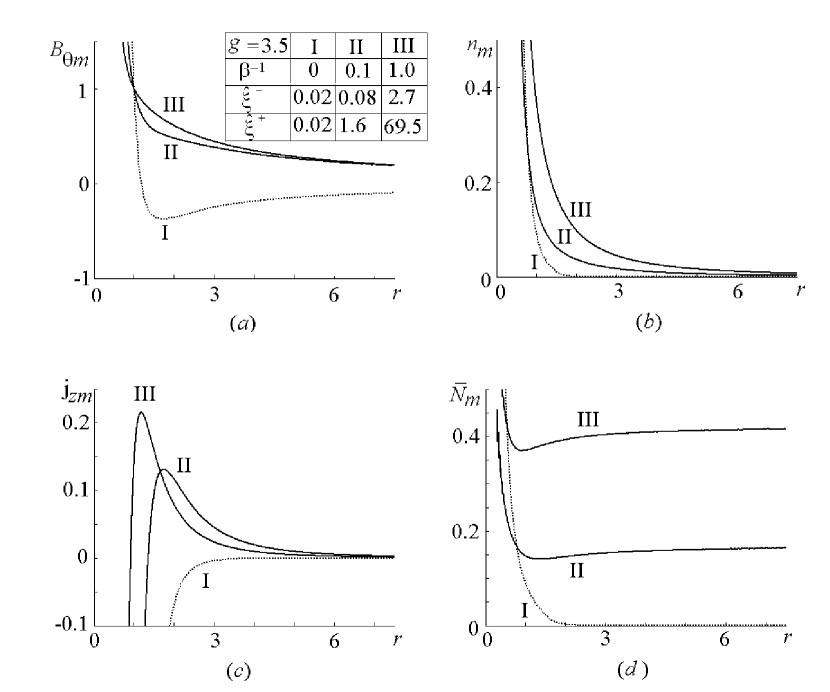
Figure 2: Equilibrium midplane profiles of the toroidal magnetic field $(a)$, number density $(b)$, distributed electric current $(c)$ and inertial moment density $(d)$ vs $r$ for $g\equiv g_{0}=3.5$ and three values of the plasma beta $\beta$ (curves I, II, III); ${\hat{\xi}}^{-}<{\hat{\xi}}\equiv{\hat{\xi}}_{0}<{\hat{\xi}}^{+}$ belongs to the region of instability.

Figure 3: Equilibrium midplane profiles of the toroidal magnetic field $(a)$, number density $(b)$, distributed electric current $(c)$ and inertial moment density $(d)$ vs $r$ for $g\equiv g_{0}=-0.8$ and three values of the plasma beta $\beta$ (curves I, II, III); ${\hat{\xi}}^{-}<{\hat{\xi}}\equiv{\hat{\xi}}_{0}$ belongs to the region of instability.

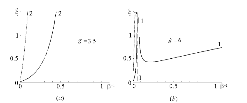
Figure 4: Marginal stability curves in the plane of the Hall criterion and inverse plasma beta $\beta^{-1}-{\hat{\xi}}$ for (a) $g=3.5$ and (b) $g=6$ ($g\equiv g_{0}>1$, ${\hat{\xi}}\equiv{\hat{\xi}}_{0}$, reference radius $r=1$ in the midplane $z=0$). Dotted/solid lines depict the upper/bottom branches ${\hat{\xi}}={\hat{\xi}}^{\pm}$ of the marginal stability curves. Dashed lines depict the asymptote I ($\partial_{r}N_{m}=0$) that separates the sub-modes 1 and 2. The upper branch in Fig. 4b and both branches in Fig. 4a for the sub-mode 1 are not presented since they correspond to the Hall parameter ${\hat{\xi}}>1.5$.

Figure 5: Marginal stability curves in the plane of the Hall criterion and inverse plasma beta $\beta^{-1}-{\hat{\xi}}$ for (a) $g=-0.8$ and (b) $g=-1.2$ ( $g\equiv g_{0}<0$, ${\hat{\xi}}\equiv{\hat{\xi}_{0}}$, reference radius $r=1$ in the midplane $z=0$). Solid lines depict the marginal stability curves. Dashed lines depict the asymptote I ($\partial_{r}N_{m}=0$) that separate the sub-modes 1 and 2, and the asymptote II ($q=0$) which restricts the region of instability for the sub-modes 2.

Figure 6: Scaled growth rate vs inverse plasma beta for (a) $g=3.5$ ($q>1$) and (b) $g=-0.8$ ($q<0$); $g\equiv g_{0}$, $\,{\hat{\xi}}\equiv{\hat{\xi}}_{0}$.

Figure 7: Dimensional characteristic toroidal magnetic field in milli-Gauss vs reference radius in astronomical units for three values of the ionization degree $\alpha$; ${\hat{\xi}}\equiv{\hat{\xi}_{0}}=0.2$; $\epsilon=0.02$ ; $n_{*}\equiv n_{n}=10^{12}cm^{-3}$; $GM=1.3\cdot 10^{-12}cm^{3}/s^{2}$ .

References

- Balbus & Hawley (1991) Balbus S. A., Hawley J. F. 1991, ApJ, 376, 214
- Balbus & Terquem (2001) Balbus S. A., Terquem C. 2001, ApJ, 552, 235
- Brushlinskii & Morozov (1980) Brushlinskii K.V., Morozov A.I. in: Reviews of Plasma Physics, edited by M.A. Leontovich, (Consultants Bureau, New York, 1980), 8, 105
- Calvet et al. (2002) Calvet N., D’Alessio P., Hartmann L., Wilner D., Walsh A., Sitk M. 2002, AJ, 568, 1008
- Desch (2004) Desch S. J., 2004, ApJ, 608, 509
- Guilloteau & Dutrey (1998) Guilloteau S., Dutrey A., 1998, A&A, 339, 467
- Hawley & Krolik (2002) Hawley J. F., Krolik J. H., 2002, ApJ, 566, 164
- Huba (1991) Huba J.D., 1991, Phys. Fluids B, 3, 3217
- (9) Kadomtzev B.B., 1976, Collective Phenomena in Plasma, Nauka, Moscow (in Russian)
- (10) Kluźniak W., Kita D., 2000, astro-ph/0006266, 1, 1
- (11) Kolberg Z., Liverts E., Mond M., 2005, Phys. Plasmas, 12, 062113
- Liverts & Mond (2004) Liverts E., Mond M., 2004, Phys. Plasmas, 11, 55
- (13) Proga, D., 2003, ApJ, 585, 406
- Papaloizou & Terquem (1996) Papaloizou J. C. B., Terquem C., 1997, MNRAS, 287, 771
- Regev (1983) Regev O., 1983 ,A&A, 126, 146
- Rudiger and Kitchatinov (2005) Rudiger G., Kitchatinov L. L., 2005, A&A, 434, 629
- Salmeron & Wardle (2003) Salmeron R., Wardle M., 2003, MNRAS, 345, 992
- Salmeron & Wardle (2005) Salmeron R., Wardle M., 2005, MNRAS, 361, 45
- (19) Sano T., Stone J. M., 2002b, ApJ, 577, 534
- (20) Sano T., Stone J. M., 2002a, ApJ, 570, 314
- Shtemler & Mond (2006) Shtemler Y.M., Mond M., 2006, J. Plasma Phys., 72, 669
- Terquem & Papaloizou (1996) Terquem C., Papaloizou J. C. B., 1996, MNRAS, 279, 767
- Umurhan et al (2006) Umurhan O. M., Nemirovsky A., Regev O., Shaviv G., 2006, A&A, 446, 1
- Urpin and Rudiger (2005) Urpin, V., Rudiger, G., 2005, A&A, 437, 23
- (25) Van Dyke M. 1964, Perturbation methods in fluid mechanics (Academic Press New York)
- Wardle (1999) Wardle M., 1999, MNRAS, 307, 849