Spectral variability analysis of an XMM-Newton observation of Ark 564

Abstract

Context. We present a spectral variability analysis of the X-ray emission of the Narrow Line Seyfert 1 galaxy Ark 564 using the data from a $\sim$ 100 ks XMM-Newton observation.

Aims. Taking advantage of the high sensitivity of this long observation and the simple spectral shape of Ark 564, we determine accurately the spectral variability patterns in the source.

Methods. We use standard cross-correlation methods to investigate the correlations between the soft and hard energy band light curves. We also generated 200 energy spectra from data stretches of 500 s duration each and fitted each one of them with a power law plus a bremsstrahlung component (for the soft excess) and we investigated the correlations between the various best fit model parameter values.

Results. The “power law plus bremsstrahlung” model describes the spectrum well at all times. The iron line and the absorption features, which are found in the time-averaged spectrum of the source are too weak to effect the results of the time resolved spectral fits. We find that the power law and the soft excess flux are variable, on all measured time scales. The power law slope is also variable, and leads the flux variations of both the power law and the bremsstrahlung components.

Conclusions. Our results can be explained in the framework of time-dependent Comptonization models. They are consistent with a picture where instabilities propagate through an extended X-ray source, affecting first the soft and then the hard photons producing regions. The soft excess could correspond to ionized disc reflection emission, in which case it responds fast to the primary continuum variations. The time scales are such that light travel times might additionally influence the observed variability structure.

1 Introduction

Ark 564 is the X-ray brightest Narrow-line Seyfert 1 (NLS1) galaxy with a 2$-$10 keV flux of $\sim 2\times 10^{-11}$ erg cm^-2 s^-1(Turner et al. 2001). From a recent deep XMM-Newton observation Papadakis et al. (2006, Paper I) found a hard X-ray power law slope of $\Gamma=2.43\pm 0.03$, in agreement with previous ASCA (Turner et al. 2001) and BeppoSAX (Comastri et al. 2001) results. The strong Fe K$\alpha$-line claimed by Turner et al. (2001) was not seen. Instead, a weak ($\sim 90$ eV) emission line, possibly from ionized iron, was detected. The presence of a soft excess was verified but neither the existence of a strong edge-like absorption feature at 0.712 keV (Vignali et al. 2004) nor the reported emission like feature at $\sim$ 1 keV (Comastri et al. 2001) could be confirmed. Instead, the soft excess is rather smooth and featureless, with the most notable feature being a broad, shallow flux deficit in the energy range $0.65-0.85$ keV, similar to the deep troughs that have been detected in the soft X-ray spectra of several Seyfert galaxies and are inferred to be “Unresolved Transition Array” (UTA) of iron $n=2-3$ absorption lines. The smooth soft excess component could equally well be fitted by a relativistically blurred photo-ionized disc reflection model or a two black body components (kT$\sim 0.15$ and $0.07$ keV) model.

Ark 564 shows large amplitude flux variations on short time scales (Leighly 1999). The source was observed for a period of $\sim 35$ days in June/July 2000 by ASCA as part of a multi-wavelength AGN Watch monitoring campaign (Turner et al. 2001).Using these data, Papadakis et al. (2002) reported a “-1 to -2” break in the power spectrum at high frequencies ($\sim 2\times 10^{-3}$ Hz). On the other hand, Pounds et al. (2001) detected a ”zero to -1” low frequency break in the PSD at $\sim 1/13$ days^-1, using long term RXTE monitoring observations. When combined together, these two results support the idea of a small black hole mass and high accretion rate in Ark 564 . Finally, using nonlinear techniques Gliozzi et al. (2002) were able to demonstrate that the source behaves differently in the high and low flux states.

Using the same long ASCA monitoring data, Edelson et al. (2002) and Turner et al. (2001) studied the spectral variability behavior of the source. Edelson et al. (2002) found that the short-timescale (hours-days) variability patterns were very similar across energy bands, and the fractional variability amplitude was almost independent of energy. Furthermore, no evidence of lags between any of the energy bands studied could be found. Turner et al. (2001) detected significant variations on the hard band spectral slope, by a factor of $\Delta\Gamma=0.27$, down to a timescale of approximately a day. Furthermore, the soft excess flux and shape were also variable down to timescales of approximately a day. The power law and soft excess fluxes were well correlated, with no delays, on time scales longer than a day.

The integrated luminosity between 10^-5 and 10 keV of Ark 564  is $\sim 10^{45}$ ergs s^-1 (Romano et al. 2004). Its black hole mass estimate of $\sim 2.6\times 10^{6}M_{\odot}$ (Botte et al. 2004) suggests that the system is accreting near its Eddington limit. Consequently, the time scales in the innermost region of the accretion disc around such a black hole are expected to be very short. For example the light travel time scale is of the order of a few $\times$ 100 s in the innermost $\sim$10 Schwarzschild radii for such a small black hole mass. Therefore, in order to probe the physical processes that operate in the innermost accretion flow we need to study the spectral variations of the source on time scales much smaller than a day. The high time resolution and good signal to noise data that XMM-Newton provides are well suited for this kind of work.

In this paper we present the results from the time resolved spectral analysis of the data from the January 2005, 100 ks XMM-Newton observation of Ark 564. Our main aim is to study the variability behavior of the continuum components in the X-ray spectrum of Ark 564 , i.e. of the soft excess and the hard band power law component. Ark 564 is an ideal target for the investigation of the continuum spectral variability on short time scales. The main reason is that, as we have shown in Paper I (where we presented the results from the analysis of the time-averaged spectrum of the source), its X-ray spectrum is almost “clean” of any significant absorption and/or emission features. Hence, it is possible to determine the X-ray continuum components with the use of simple phenomenological models, without significant uncertainties associated with the presence of features due to (warm and/or cold) absorbing/emitting material in the source.

A detailed timing analysis, focusing on the study of the phase lags and the coherence as a function of Fourier frequency, has been presented by Arevalo et al. (2006), while McHardy et al. (2006) will present the result from a detailed timing analysis based on power spectral analysis methods.

The present work is organized as follows: After a brief description of the observation we present in Sect. 3 the timing analysis of the light curves, both with conventional techniques as well as with a sliding window approach. In section 4 we describe the time resolved spectral fits and the correlations of the obtained spectral parameters as well as the correlations of the fluxes of the different components in different energy bands. We close in section 5 with a discussion of the obtained results.

2 Observation and Data Analysis

Ark 564 was observed with XMM-Newton from 2005 January 5, 19:47 to 2005 January 6, 23:16 for about 10⁵ s. The PN camera and the two MOS cameras were operated in Small Window mode with a medium thick filter. For the current analysis we will use only the PN data. The data were reprocessed with the XMMSAS version 6.5 and for the spectral analysis the most recent versions of the response matrices were used.

The background count rate was very low (in total less than 0.6% of the source count rate), apart from two small, short flares at the beginning of the observation. Data from these periods were disregarded from the spectral analysis.

With an average count rate of $\sim$ 30 cts s^-1 photon pile-up is negligible for the PN detector, as was verified using the XMMSAS task $epatplot$. Source counts were accumulated from 27$\times$26 RAW pixels around the position of the source; the background data were extracted from a similar, source free region on the chip. We selected single and double events for the analysis (PATTERN$\leq 4$ and FLAG=0; for details of the instruments see Ehle et al. 2005) in the energy range from 300 eV to 12 keV. In total $\sim$ 2$\times 10^{6}$ photons were accumulated in an integration time of $\sim$ 69300 s.

3 Light curve timing analysis

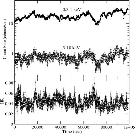
Figure 1: Background subtracted PN light curves of Ark 564 in the 0.3$-$1 keV (filled dots) and 3.0$-$10 keV (open circles) energy bands. Note that in reality the count rates are larger, as the data have not been corrected for the 71% life time of the Small Window mode of the detector. Bottom panel: hardness ratios between hard and soft band light curves. The time binning is 100 s.

We start our study by examining light curves in “soft” and “hard” bands. The advantage of this approach is that it is model independent, however it has also its limitations, as it is difficult to disentangle the interplay between the various spectral components in each energy band. Fig. 1 shows the PN 0.3$-$1 keV and 3$-$10 keV background subtracted light curves, binned in 100 s intervals. We consider the light curves in 3$-$10 keV and 0.3$-$1 keV as representative of the “hard” and “soft” energy bands, respectively. The high energy band range has been chosen to minimize the contribution of the soft excess emission component which becomes apparent at energies below $\sim 2$ keV (Paper I). The contribution of this component is significant in the soft energy band light curve. However, as the hard power law very likely continues into this band, the interpretation of the observed variations in this band is difficult.

The source is highly variable on all sampled time scales in both energy bands. The max/min variability amplitude is of the order of $\sim 6$ and 4 in the hard and soft band light curves, respectively. The fractional variability amplitude (corrected for the experimental noise) in the hard energy band is $f_{\rm rms,hard}=27.1\pm$ 0.4%, as opposed to $f_{\rm rms,soft}=24.7\pm 0.1$% in the soft band light curve. Errors account only for the measurement error of the light curve points, and have been estimated according to the prescription of Vaughan et al. (2003). This difference in the variability amplitudes suggest the presence of spectral variations which can be seen in the lower panel of Fig. 1 where we plot the hardness ratios (HR), i.e. the ratio of the hard to the soft band light curves. A $\chi^{2}$ test shows that the HR light curve is indeed significantly variable ($\chi^{2}=3464/988$ degrees of freedom - dof). The fractional variability amplitude of the HR light curve is $f_{\rm rms,HR}=17.9\pm 0.4$%, suggesting that the amplitude of the spectral variations is lower than that of the flux variations in both the soft and hard band light curves.

3.1 Cross-Correlation Analysis

In order to investigate the cross-links between the hard and soft band light curves we estimated their cross-correlation function (CCF), using light curves with a 100-s bin size. We calculated the sample Cross-Correlation Function, $CCF(k)$, as follows:

$$CCF(k)=\frac{\sum_{t}(x_{soft}(t)-\bar{x}_{soft})(x_{hard}(t+k)-\bar{x}_{hard})}{N(k)(\sigma^{2}_{soft}\sigma^{2}_{hard})^{1/2}},$$

$$k=0,\pm\Delta t,\ldots,\pm(N-1)\Delta t.$$

The summation goes from $t=\Delta t$ to $(N-k)\Delta t$ for $k\geq 0$ ($\Delta t=100$ s, and $N$ is the total number of points in the light curve) and the sum is divided by the number of pairs included, i.e. $N(k)$. For negative lags $k<0$ the summation has to be done over x${}_{\mathrm{s}oft}(t+|k|)$ and x${}_{\mathrm{h}ard}(t)$. The variances in the above equation are the source variances, i.e., after correction for the experimental variance. Significant correlation at positive lags means that the soft band variations are leading those in the hard band.

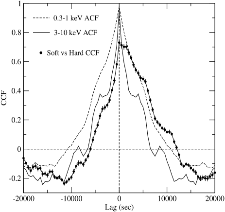
Figure 2: Autocorrelation functions of the soft and hard band data and the cross-correlation function between the soft and the hard light curve. The time binning is 100 s. Positive lags mean that the hard variations are lagging behind the soft.

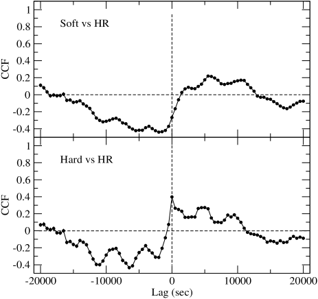
Figure 3: Cross-correlation function between the HR and the the soft - hard band light curves (upper and lower panels, respectively).The time binning is 100 s. Positive lags mean that the HR spectral variations are lagging behind the flux variations.

First, we computed the auto-correlation function (ACF) of the hard and soft band light curves and the CCF (up to lags $\pm 2\times 10^{4}$ s) using the whole length (i.e. the total) light curves. In Fig.2 we show the soft and hard band ACFs (continuous and dashed lines, respectively) and their cross-correlation function (filled circles).

The maximum CCF amplitude reaches a value of $\sim$ 0.7, at zero lag. This result implies that the soft and the hard band light curves are well correlated. This is not surprising, given the fact that the two light curves look very similar (see Fig. 1), with most of the variability patterns, on all time scales, appearing in both of them. Furthermore, the CCF appears to be highly asymmetric with higher values appearing at positive lags. The asymmetry of the hard vs soft CCF becomes immediately apparent if we compare it with the respective ACFs. This result implies complex delays between the hard and the soft band light curves. It is in agreement with the results of Arevalo et al. (2006) who also find that the variability components in the 0.7$-$2 keV are leading those in in the 2$-$10 keV band. However, the time delay between the variations in the two bands is not constant, but rather decreases with increasing period of the Fourier components. In this case, broad, asymmetric towards positive lags CCFs are expected, like the one shown in Fig. 2.

The cross-correlation between the soft and hard band light curves and the hardness ratios (Fig.3) is rather weak at all lags. The “strongest” signal appears at negative lags which implies that the flux variations may be weakly anti-correlated with the HR variations with a delay of $\sim 2-$5 ks. If real, this anti-correlation between the soft and hard band fluxes and the hardness ratio is hard to explain given the possible contribution of both the strong soft excess and the power law component in the soft band light curve of this object.

3.2 Sliding window CCFs

The CCFs shown in Figs. 2 and 3 represent the average correlation structure between the two light curves, originating from the integration over the total length of the observation. Recently, Brinkmann et al. (2005) employed the “sliding window” technique in the study of the CCFs between various energy bands in the case of the BL Lac object Mrk 421. As is typical of objects in the same class, Mkn 421 shows well defined flare-like events in its light curves, with different variability characteristics. As a result, the use of this method revealed that the cross-correlation structure also evolves during each individual events.

In order to investigate in more detail the cross-correlation between the soft and hard band variations, over shorter time periods we employed the same “sliding window” technique and calculated the CCFs for shorter data intervals, which start at different times of the observed light curve and range over a restricted time interval. Thus, the above defined CCF(k) is replaced by a CCF(k; $\mathcal{T,L}$), i.e., the cross-correlation coefficient at a lag ‘k’ is calculated for a data stream with length $\mathcal{L}$ which starts at the time $\mathcal{T}$ in the light curve. Details of the method and the choice of an optimal window length $\mathcal{L}$ which reveals best the “time evolution” of the CCF structure are given in Brinkmann et al. (2005).

In Fig. 4 we show a two dimensional representation of the sliding window CCFs, based on light curves with 10 s binning. The vertical scale represents the lags (similar to the x-axis of Figs. 2 and 3), the color coding indicates the amplitude of the cross-correlation coefficient, with the color code given in the lowest panel of the figure. Time is along the x-axis. The two upper panels show the cross-correlation function between the soft and hard band light curves for two window lengths, $\mathcal{L}$ = 10 ks and $\mathcal{L}$ = 19 ks.

Clearly visible is the temporal sub-structure in the CCFs, which gets averaged out for the longer window lengths and approaches, finally, the “global” averages seen in Fig.2. During the period of “low-amplitude” activity (i.e. between $\sim 20$ and $\sim 60$ ks after the start of the observation) the CCFs are of lower amplitude and peak around zero lag. During the first and last part of the observation though, the CCF has a larger amplitude and peaks at positive lags, between $\sim 0-2$ ks. The main result of this analysis is that there exist strong correlations only at zero or positive lags. This is in contrast to, for example, Mrk 421 where lags with changing signs have been observed (e.g. Brinkmann et al. 2005).

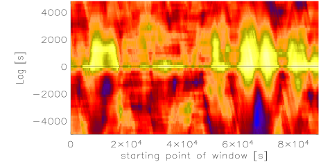
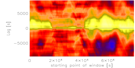
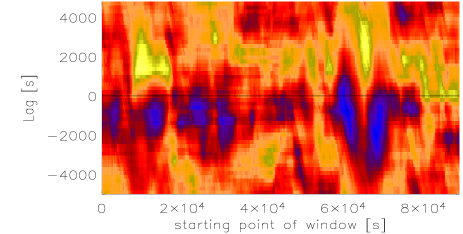
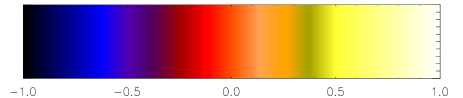
Figure 4: Sliding window CCFs between soft and hard band fluxes (upper panel with window length $\mathcal{L}$ = 10 ks, middle panel with window length $\mathcal{L}$ = 19 ks). In the lower panel we plot the sliding window CCFs ($\mathcal{L}$ = 10 ks) between the soft flux and the hardness ratios. The amplitude of the CCF is color coded, with lags plotted in the vertical direction. The bottom panel shows the color bar used for the numerical values of the CCFs.

The third panel of Fig. 4 shows the sliding window CCFs between the soft band flux and the hardness ratios. The length of the data sets is again $\mathcal{L}$ = 10 ks. Overall, the correlation between these quantities is rather low, at all times. During the “low-amplitude” activity period (i.e. during the middle of the observation) we cannot detect any correlation between the two light curves, most probably due to the low amplitude variations. Towards the end and at the beginning of the observation, we detect the signals at positive and negative lags of $\sim 2$ and $\sim-2$ ks, respectively. In both cases though, the positive and negative lag “signals” are of low amplitude (i.e. CCF${}_{\rm max}\leavevmode\nobreak\ \raise 2.15277pt\hbox{$<$}\kern-8.00003pt\lower 2.84526pt\hbox{$\sim$}\leavevmode\nobreak\ 0.5$).

In order to proceed and to investigate further the correlation between the flux and spectral variations in Ark 564   we need to disentangle the contribution of the hard and soft spectral components in the soft energy band. This can be achieved by model fitting to the energy spectra acquired over short periods of time. In the section below we present the results from this temporally resolved spectral analysis.

Before proceeding, it is worth mentioning that one of the main results from the “sliding window” CCF analysis is that the “global” cross-correlation properties between the light curves in the two energy bands are mainly defined by the “signals” we detect at the beginning and towards the end of the observation (i.e. during the first $\sim 20$ ks and in the period between 60 and 80 ks after the start of the observation). In the first period we observe a steady flux increase (by a factor of $\sim 2-3$) and then a much shorter flux decline (over a period of less than $\sim 2-3$ ks), reminiscent of a flare-like event. In the second period, we observe a long ($\sim 10$ ks), well defined flux decay (by a factor again of $\sim 2-3$) and a subsequent flux rise over a similar time scale. These are the most prominent, long, well defined “features” in the observed light curves (see Fig. 1). In the periods between these two main “events”, the flux variations are of lower amplitude and are less well defined. Hence it is harder to detect strong cross-correlation signals. In the analysis presented in the following sections, we pay particular attention to these two periods which show the strongest cross-correlation signals between the soft and hard band light curves.

4 Time resolved spectral fitting analysis

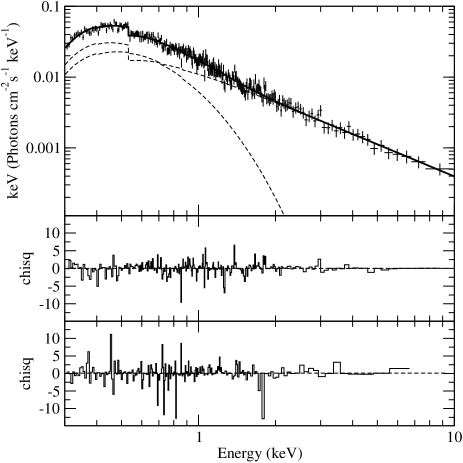
Figure 5: Plot of a good power law plus bremsstrahlung fit (upper panel) and of the respective residuals (middle panel) to the PN data in the $0.3-10$ keV energy band. The lower panel shows the residuals of the worst fit obtained.

As the count rate of the Ark 564 XMM-Newton observation is sufficiently large, we split up the total exposure into 200 individual data stretches of 500 s duration each, and generated the energy spectrum in each of them. Each of the thus obtained spectra has   $>$$\sim$   10000 photons in the $0.3-10$  keV band, sufficient for the accurate determination of the parameters of the relatively simple spectral models that we use. All model fits were done using XSPEC v. 11.3, and in all cases we fixed the interstellar absorption at the galactic value of N_H,Gal = $6.4\times 10^{20}$ cm^-2 (Dickey & Lockman 1990). In all cases we use the 1$\sigma$ errors for one interesting parameter.

A simple power law (PL) model fits the $3-10$ keV band of all these spectra very well. However, it cannot provide an acceptable fit to the full $0.3-10$ keV band. A soft excess emission component is always present at energies below $\sim 1.5$ keV. We investigated whether a combination of just two spectral components could fit the entire $0.3-10$ keV band. We used a combination of a PL plus a black body or a PL plus a bremsstrahlung (PL+Brems) model and found that the second combination fits most of the 500 s spectra significantly better. It results nearly always in an excellent fit: the mean reduced $\chi^{2}$ of all 200 fitted spectra is $<\chi^{2}_{\rm red}>$ = 1.0024, with a variance of $\sigma=0.0068$.

In Fig. 5 we show one of the best PL+Brems fits to one of our 500 s data stretches ($\chi_{\rm red}^{2}=$ 0.951 / 279 dof) and the corresponding $\chi^{2}$ plot (top and middle panel, respectively). In the bottom panel, we plot the $\chi^{2}$ plot of the worst fit we obtained ($\chi_{\rm red}^{2}=$1.31 / 217 dof). In both cases the resulting quality of the fits is determined by the scatter of individual data bins. There are no obvious systematic deviations between data and the model, suggestive of the presence of any extra spectral components that we should consider.

In particular, none of the absorption and emission features that were detected in the time-averaged spectrum of the source (i.e. the weak iron emission line at $\sim 6.7$ keV, the absorption line at $\sim 8$ keV, and the broad, but shallow, flux deficit at $\sim 0.7-0.9$ keV; see Paper I) showed up in the spectra which are extracted from the shorter data intervals, due to the limited photon statistics.

In order to investigate this issue better, we fitted again the lowest, highest flux, and the worst-fit 500 sec spectra with a PL+Brems model plus 1) a DISKLINE and Gaussian absorption line component (using the model parameter values listed in the PN, PL+DL+ABL model fitting results of Table 1 in Paper I) and 2) the four Gaussian lines that we used to model the absorption in the Fe UTA region. The best fitting PL and Brems model results were almost identical to the values we obtain when we do not consider the small amplitude absorption/emission features in the time-averaged spectrum of the source.

We repeated the same procedure for 20 more, randomly chosen 500-sec long spectra. In all cases, the addition of model components that correspond to the absorption and/or emission features in the time-averaged spectrum of the source does not affect at all the continuum (i.e. PL and Brems) model fitting results.We conclude that the PL+Brems model can fit well the time resolved spectra, over the entire 0.3$-$10 keV band. Consequently, we decided to use the results from the PL+Brems model fitting to the spectra as the basis for our study of the spectral variability properties of the source.

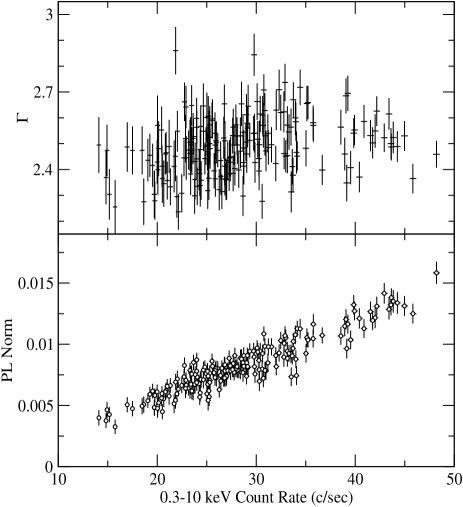
Figure 6: Left: Best fitting power-law index (upper panel) and power-law normalization (lower panel) values plotted as function of the observation time. Right: The same parameters are plotted as a function of the 0.3$-$10 keV count rate.

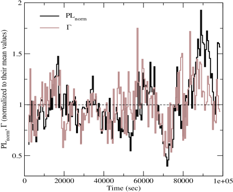
Figure 7: Power law normalization (black) and and amplitude adjusted power law slopes (grey), both normalized to their mean values, shifted in time by + 2 ks.

4.1 Best fitting power-law parameter correlations

The left panel of Fig. 6 displays the best fitting values for the PL spectral slope and normalization as function of the observing time. In the right panel of the same figure, we show these parameter values as a function of the 0.3$-$10 keV count rate.

The PL normalization (PL_norm) varies substantially, and these variations are obviously the primary cause of the sources’ variability. As the right hand bottom panel of Fig. 6 confirms, there exists a very strong, linear correlation between the observed count rate and PL_norm. The max-to-min variability amplitude of $\sim$ 4.8 in the observed light curve can almost entirely be explained by the PL_norm variations.

The power law spectral slope is also variable, but at a smaller level. Its average value is $<\Gamma>=2.488\pm 0.005$, similar to best PL model fitting to the hard band of the time-averaged spectrum, reported in Paper I. The individual PL slopes vary between $\sim 2.3-2.7$, with an average amplitude of $f_{\rm rms,\Gamma}=3.3\pm 0.2$%, much smaller than that of the PL_norm ($f_{\rm rms,PLnorm}=26.0\pm 0.6$%). On the top right hand panel, we plot $\Gamma$ as a function of total observed count rate. There might exist a weak correlation, possibly with a slightly different behavior at highest fluxes, but the large uncertainty associated with the $\Gamma$ measurements does not allow us to draw any firm conclusions.

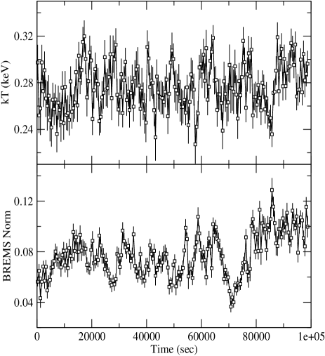
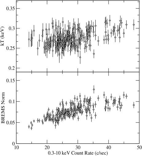
Figure 8: Left: Best fitting temperature (upper panel) and the corresponding normalization values (lower panel) of the bremsstrahlung component plotted as function of the observation time. Right: The same parameters plotted as function of the 0.3$-$10 keV count rate.

Despite the difference in the variability amplitudes, $\Gamma$ and PL_norm are well correlated. Interestingly, there also appears to be a time delay between the variations of these two parameters. As an illustrative example we have drawn two dashed lines in the left hand panels of Fig. 6. They indicate the high and low PL_norm values $\sim 17$ ks and 70 ks after the beginning of the XMM-Newton observation, respectively. The associated $\Gamma$ variations are clearly leading those in the PL_norm light curve, by about 1-2 ks.

The good correlation between PL_norm and $\Gamma$ is further demonstrated in Fig. 7 which shows $\Gamma$ and PL_norm plotted as a function of time. Both curves are normalized to their mean. The normalized $\Gamma$ values are furthermore scaled by a factor of 5, and shifted by + 2 ks. Visible is the overall excellent correlation between the two quantities. However, there also exist some subtle anti-correlations and mismatches, for example at $\sim 20,45-55,$ and 77 ks after the observations start. Some of them could be the result of the fact that the delay between the variations in the two parameters is not exactly equal to 2 ks. Towards the end of the observation (  $>$$\sim$   85 ks since its start), the correlation ceases to be good, with a prominent “flare-like” event in the PL_norm vs time plot, which is almost absent in the respective $\Gamma$ vs time curve.

4.2 Best fitting bremsstrahlung parameter correlations

Figure 8 shows the corresponding results of the bremsstrahlung component. On the left hand side panels, we plot the best fitting kT (upper panel) and bremsstrahlung normalization values (brems_norm; lower panel) as function of time. In the right hand panels, we plot the same parameter values as a function of the total count rate.

The bremsstrahlung normalization is variable, with an average variability amplitude of $f_{\rm rms,brems-norm}=20.0\pm 0.6$%. This result shows clearly that the soft excess component is variable in Ark 564. In fact, our results demonstrate that this component is variable on time scales as short as a few hundred seconds. Its variability amplitude is smaller than that of the PL_norm, and of the observed full band light curve. Nevertheless, as with PL_norm, brems_norm follows rather closely the intensity variations. The correlation between brems_norm and count rate (as implied by the right hand bottom panel in Fig. 8) is rather good, although with substantial scatter, indicative of the strong influence of the PL component variations in the intensity variations that we observe. There is also an indication that at the highest count rate level the normalization of the soft component may saturate at a constant value.

Visual inspection of the bottom left hand panels in Figs. 6 and 8 reveals that brems_norm and PL_norm are well correlated. The cross-correlation analyzes of the two light curves in these panels does indeed show a maximum of $\sim 0.7$ at a lag of $\sim 0.5-1$ ks, indicating that the PL_norm variations may be slightly delayed with respect to the brems_norm variations. Furthermore, the visual inspection of the top and bottom left hand panel in Figs. 6 and 8, respectively, suggests that brems_norm is also correlated with $\Gamma$. A cross-correlation analysis results in a CCF_max value of 0.5, at a lag of $\sim 1-5$ ks. In other words, just like the PL_norm, the brems_norm variations are delayed with respect to the PL spectral slope variations.

Finally, we find that the bremsstrahlung temperature is also variable. A $\chi^{2}$ test results in $\chi^{2}=422.1/197$ dof. The kT variations are of low amplitude with $f_{\rm rms,{\rm kT}}=4.9\pm 0.7$%, similar to the PL slope variability amplitude. However, they do not correlate, at any lag, neither with brems_norm nor with PL_norm, $\Gamma$ or the observed intensity variations.

In summary, our results so far show that: a) Both the PL normalization and slope are variable, on time scales as short as $0.5-1$ ks, b) The soft excess component is variable on short time scales, mainly in amplitude, c) the observed flux variations in the soft and hard energy band light curves are mainly caused by the PL and the soft excess component normalization variations, d) the PL and bremsstrahlung normalization variations are well correlated, with no delays, and finally, e) the spectral slope variations seem to lead (by $\sim 1-2$ ks) the PL and bremsstrahlung normalization variations.

The final step in the investigation of the spectral variations of the source is to use the best fitting spectral parameter values to determine the fluxes of the individual components in various energy bands, and then their cross-correlations.

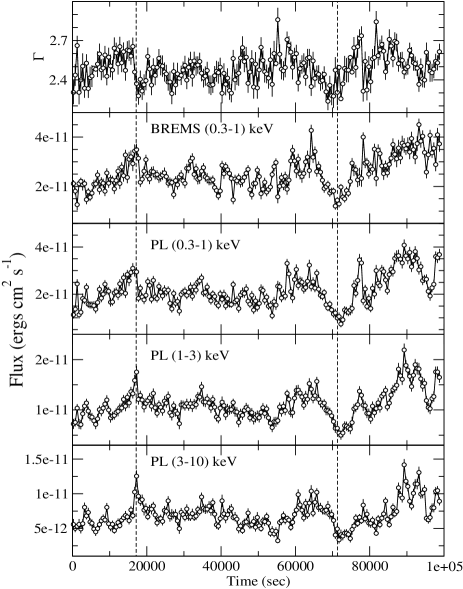
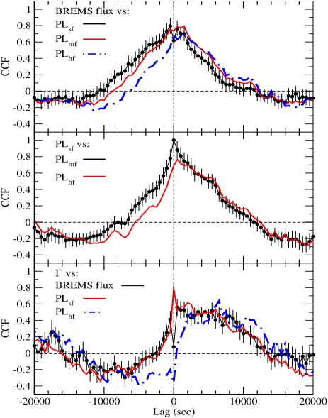
Figure 9: Left: The PL best fit spectral slopes (top panel), the bremsstrahlung $0.3-1$ keV flux (second panel from top), the power law $0.3-1$ and $1-3$ keV flux (third and fourth panel from top), and the $3-10$ keV flux (bottom panel), plotted as a function of time. Right: Cross-correlation functions between the various parameters which are plotted on the left side.

4.3 Flux-flux correlations

Fluxes provide a more direct tracer of the sources’ emission characteristics than the count rates which are subject to short term spectral variations and the folding with the detector response. For example, comparing the total 0.3$-$10 keV light curve with the calculated fluxes we find differences around   $<$$\sim$   1% in a 500 s bin. This is, however, only a lower bound for the high energy band as most of the flux / count rate is found in the soft band.

In the left hand panel of Fig. 9, we plot the bremsstrahlung $0.3-1$ keV flux, and the PL $0.3-1$, $1-3$ and $3-10$ keV fluxes (PL_sf, PL_mf, and PL_hf, respectively) as a function of time. In these plots the estimated errors of the fluxes are generally smaller than the symbol sizes. The fractional variability amplitude is $f_{\rm rms,brems}=23.8\pm 0.01$%, $f_{\rm rms,PL_{sf}}=29.5\pm 0.01$%, $f_{\rm rms,PL_{mf}}=24.5\pm 0.01$%, and $f_{\rm rms,PL_{mf}}=25.1\pm 0.01$%. The bremsstrahlung flux light curve shows the smallest amplitude variations, although the differences are not large.

As before, to ease the visual comparison between them, we have drawn two dashed lines to mark the two “major” events during the first 20 ks of the observation, and around 70 ks after its start. In this case, it is hard to judge whether there are any delays between the times that the various band flux light curves reach their maximum and minimum values, respectively.

However, what is clear is that there are differences in the shape of the light curves. While the bremsstrahlung flux increases steadily for the first $\sim 17$ ks, and then decays sharply within a couple of thousand seconds, the PL flux light curves show a different behavior. The difference is enhanced as the energy separation increases. For example, the PL_hf light curve increases sharply within $\sim 2$ ks before the bremsstrahlung flux maximum, and then decays smoothly over a period of $\sim 5$ ks. The same behavior is observed in the second “event”. The bremsstrahlung flux decays smoothly for over a period of $\sim 5-6$ ks before reaching its minimum and then rises steadily immediately after that. The PL_hf flux on the other hand decays much faster (within $\sim 2$ ks), and then increases at a much slower rate.

These differences in the rise and decay time scales between the various light curves are bound to introduce “delays” between the observed variations. Indeed, on the top right hand panel of Fig. 9, we show the CCF between the bremsstrahlung and the PL_sf, PL_mf, and PL_hf light curves. The bremsstrahlung flux vs PL_sf CCF shows a maximum at almost zero lag. However, the bremsstrahlung vs PL_hf and vs PL_hf CCFs are heavily skewed towards positive lags, with broad maxima at lags $\sim 0-2$ ks. These “delays” are caused to a large extend by the differences in the rise and decay time scales of the “flares” in the respective light curves.

In the middle right hand panel of Fig. 9 we plot the PL_sf vs PL_mf and the PL_sf vs PL_hf cross-correlation functions. In agreement with the CCFs plotted in the panel above, they also look asymmetric, and shifted to positive lags. As before, these “delays” are mainly caused by the differences in the shape of these light curves.

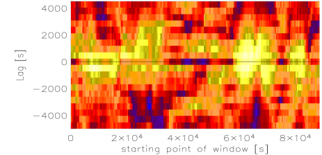
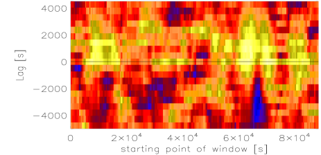
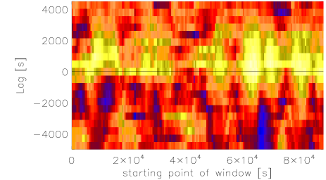
Figure 10: Sliding window CCFs between the bremsstrahlung and soft power law flux (upper panel), between bremsstrahlung and hard power law flux (middle panel) and between soft and hard band power law fluxes (lower panel). The time binning is 500 s, the window length $\mathcal{L}$ = 10 ks; color coding and description as in Fig. 4.

The lower than unity CCF maximum values are caused by the fact that the correlation coefficient changes on time scales of a few ks. This is demonstrated in Fig. 10 which shows on top the sliding window CCF of the bremsstrahlung and the soft power law flux. The correlation coefficient changes with time and shows its maxima at the two major flux variations events we have discussed before. In between, most probably the low amplitude variations do not allow us to pick any significant signals. In the middle and bottom panels we show the sliding window CCF of the bremsstrahlung and the medium power law flux and the soft vs hard power law flux, respectively. In both cases, the variations in the softer energy band lead those in the higher energy band. The maximum CCF signals appear at the two prominent flux variability events, while no significant signals appear in between.

4.4 Spectral slope vs Flux correlations

The top left hand panel of Fig. 9 displays the power law slope $\Gamma$ as a function of time. The curve looks roughly similar to the flux light curves, shown below, although it is not as variable. Looking again at the two main “events” that we have mentioned above, it now becomes clear that the $\Gamma$ variations are leading the flux variations of both the bremsstrahlung and PL components, in all energy bands.

In the bottom right hand panel of Fig. 9, we show the CCF between $\Gamma$ and the bremsstrahlung, the PL_sf, and the PL_hf flux light curves. They all show broad maxima shifted towards positive lags. The degree of the asymmetry increases with increasing energy, and is maximal in the $\Gamma$ vs PL_hf CCF. This result demonstrates clearly that in Ark 564 the PL spectral slope variations are leading the flux variations.

The CCF maximum values are rather low, being roughly equal to $0.6$. This, together with broadness of the CCFs and their “noisy” structure can be explained by the fact that, on closer inspection, the $\Gamma$ and flux variations are not always in phase (see also Fig. 7), especially towards the end of the observation where $\Gamma$ remains roughly constant and does not follow the flux variations. Furthermore, as before, the sliding window CCFs (Fig. 11) shows that changes in the power law index $\Gamma$ and the bremsstrahlung/power-law flux are intimately related during the two major variability events, but in other times the signal simply fades away.

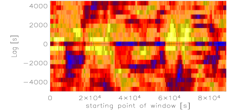
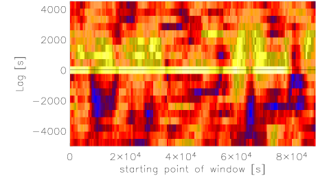
Figure 11: Sliding window CCFs between the photon index $\Gamma$ and the bremsstrahlung flux (upper panel) and between $\Gamma$ and the soft power law flux (lower panel). Color coding and description as in Fig. 4.

5 Discussion

In this paper we present the results from a detailed spectral variability study of Ark 564 using the data from a recent, 100 ks long, XMM-Newton observation of the source. We have estimated the cross-correlation functions between the soft and hard energy band light curves, and between these light curves and conventional hardness ratios. Furthermore, due to the high signal-to-noise ratio of the data, we were able to extract high quality, individual spectra from data stretches of 500 s each. We were able to study, for the first time in the case of Ark 564 , the spectral variability properties of the source down to a time scale as short as 500 s, by fitting a power law plus bremsstrahlung model to these spectra.

Ark 564 is an ideal AGN for a spectral variability investigation. First of all it is highly variable (i.e. it displays large amplitude variations on short time scales), and bright, hence we are able to probe accurately its high frequency variations. Furthermore, as we have shown in Paper I, its X-ray spectrum is almost “clean” of any significant absorption and/or emission features. For example, the top panel of Fig. 12 in Paper I demonstrates that the fraction of any manifestations of a warm absorber is no more than $4$% percent of the X-ray continuum flux in the energy band between $\sim 0.7-0.9$ keV. Furthermore, the comparison of the time-averaged spectrum of the source with that of 3C 273 (shown in Fig. 8 of Paper I) shows clearly that the overall spectrum of Ark 564 is smooth and is mainly characterized by broad continuum spectral components, which are unaffected by strong absorption and/or emission features. As a result, it is possible to determine the X-ray continuum with the use of simple phenomenological models, without any ambiguity arising from the presence of significant distortions due to strongly absorbing and/or emitting components and subsequently study its variations even on time scales as short as a few hundred seconds.

We use a simple PL model to account for the emission above 3 keV of the source. This fits well all the spectra, but only as long as $\Gamma$ varies by up to $\sim 0.4$. There have been cases in the past few years where the observed spectral variations of a few sources have been interpreted in terms of a “two-component” model (i.e. Ponti et al. 2006, and references therein). According to this model, the observed flux variations are caused by a constant-slope power law which varies in normalization only. The spectral shape variations are artificial and are introduced by the interplay of this and a second spectral component (usually attributed to ionized reflection by the disc) which is almost constant (in flux and shape). To test this hypothesis in the case of Ark 564 , we fitted the lowest and highest flux source spectra with a PL plus the ionized reflection model REFLION of Ross & Fabian (2005). We kept the values of the reflection component parameters fixed to those found in Paper I (as this component is supposed to be constant). The source spectra above 1 keV can be fitted well by this model (at lower energies, we need and extra spectral component to fit the high flux spectrum, just like in the case of the time-averaged spectrum). However, this is possible only if the PL slope changes by a factor of 0.6$\pm 0.13$. This is comparable (in fact, even slightly larger) to the $\Delta\Gamma$ we detect when we parameterize the spectra with the simple PL+bremsstrahlung model. We believe that the detected spectral slope variations in the hard band of Ark 564 are an intrinsic property of the source.

Regarding the soft band spectrum, we have used a simple bremsstrahlung law to account for the soft excess emission of the source. This does not imply that we believe the soft-excess component is indeed bremsstrahlung emission from a hot plasma (see below). However, to the extend that a variable PL component fits well the 3-10 keV band and extends to slower energies as well (as is shown by the study of the time-averaged spectrum in Paper I) then the facts that: a) the soft X-ray continuum is smooth and almost featureless and b) the bremsstrahlung model fits it well, guarantee that the flux estimates (at least) of the soft component must be similar to what we find, irrespective of what models one may use to fit the data.

In Paper I the possible detection of an absorption line at $\sim 8.1$ keV in the time average spectrum of the source was discussed. If real, this would suggest the presence of highly ionized out-flowing gas with a column density of $\sim 10^{23}$ cm^-2. Significant variations in the column density, covering factor and/or ionization state of the gas could result in spectral variations, even at energies above $2-3$ keV.

We fitted some of the 500 s long spectra with a “power law plus Brems plus ABSORI” model but it was not possible to constrain both the N_H and ionization parameter ($\xi$) of the gas. Even when N_H was kept frozen to a constant value, the uncertainty on $\xi$ was very large.

To investigate then the possible effects of $\xi$ variations we used the XSPEC command FAKE and created synthetic PN spectra (500 s long each) assuming a PL plus a bremsstrahlung and an ABSORI model component with N${}_{\rm H}=10^{23}$ cm^-2. The PL and Brems normalizations as well as the $\xi$ values were varied and the resulting spectra were fitted with a power law for energies above 2 keV. Due to the limited signal to noise of the 500 s spectra, they could all be well fitted by the PL model.

It seems that the gas must be higher ionized than what the model’s upper limit of $\xi=5000$ implies (due to the presence of model spectral features in the soft energy band which we do not observe in reality), but it is not certain whether $\xi$ variations will then result in significant $\Gamma$ variations. Nevertheless it seems not impossible that $\xi$ variations can cause spectral variations similar to what we observe in Ark 564 . We did not consider the cases of N_H or covering fraction variations, as the probability that these parameters vary on time scales as short as less than an hour is rather small.

However, our results regarding the flux variations in various energy bands and their correlations (see Sec. 4.3) should not depend on the model chosen to fit the 500 s long spectra, as long as it fits them well. It further seems rather difficult to explain why the $3-10$ keV band flux variations should be delayed with respect to the $1-3$ keV band variations if most of the spectral variations are caused by changes in the properties of the warm absorbing material, which should affect the whole spectrum simultaneously. It is also difficult to understand in this case why variations of the slope $\Gamma$ would lead the flux variations in all bands.

In summary, we believe that most of our results, which we summarize below, do not depend on the choice of the models we have used to parameterize the source’s spectral variations and that they are representative of the intrinsic properties of the source’s emission components. In particular, the results regarding the flux variations in various energy bands and their correlation with the observed spectral shape variations do not depend on the way we model the source’s spectrum.

5.1 Summary of the results

Our findings can be summarized as follows:

1) The soft ($0.3-1$ keV) and hard ($3-10$ keV) band light curves are well correlated at zero lag. The CCF is asymmetric, indicating that the hard band photons are delayed, in some way, with respect to the soft band photons.

2) The hard/soft band ratio is variable, but its variations are not well correlated with those observed in the individual light curves.

The first result is consistent with the results of Arevalo et al.  (2006), who use cross-spectral techniques to study in detail the correlation between the soft and hard band light curves. However, the interpretation is difficult because both the soft and hard band spectral components may contribute to the soft band light curve. Our time resolved spectral analysis can resolve this issue. The results from the application of this method to the Ark 564  data are as follows:

3) The shape of the hard band spectrum changes significantly on time scales as short as $\leavevmode\nobreak\ \raise 1.72221pt\hbox{$<$}\kern-6.40002pt\lower 2.84526pt\hbox{$\sim$}\leavevmode\nobreak\ 1$ ks. These changes can be well described by power law slope changes of the order of $\Delta\Gamma\leavevmode\nobreak\ \raise 1.72221pt\hbox{$<$}\kern-6.40002pt\lower 2.84526pt\hbox{$\sim$}\leavevmode\nobreak\ 0.4$, maximum.

4) An excess emission above the extrapolation of the PL model to energies down to $0.3$ keV is always present. A bremsstrahlung model fits this component well at all times.

5) The soft excess flux is significantly variable, even on the shortest time scales of $\sim 0.5-1$ ks that we can probe.

6) The PL and bremsstrahlung normalization variations are the prime drivers of the observed intensity variations of the source. The variations of the two components are well correlated with each other.

7) The bremsstrahlung $0.3-1$ keV, and the PL $0.3-1$, $1-3$, and $3-10$ keV flux light curves have different “shapes”. The rise and decay time scales decrease with increasing energy. Consequently, the PL, $3-10$ keV flux light curve is delayed with respect to both the bremsstrahlung and the PL, $0.3-1$ keV flux light curves. This result explains the CCF results between the $0.3-1$ keV and $3-10$ keV band light curves. And, finally,

8) The $\Gamma$ variations are always preceding those in the bremsstrahlung and PL component flux light curves. The delays increase with increasing energy. Such a result could not be detected in the CCF between the hardness ratio and the intensity light curves, because, as it is defined, the hardness ratio is not representative of the slope of the PL component.

We discuss below some possible implications of these results in the context of a few current theoretical models.

5.2 Comptonization models

It is widely accepted that the high energy, X-ray power law continuum in AGN is produced in a hot corona which is located above the accretion disc by Comptonization of soft thermal photons (e.g. Haardt & Maraschi 1993, Haardt et al. 1994). This model is in particular attractive for NLS1 galaxies as reflection features (like the iron line) tend to be more suppressed by Compton scattering in the corona itself (Matt et al. 1997), and a magnetically heated corona, where the energy is primarily stored in magnetic fields which reconnect and release their energy in flares (Merloni & Fabian 2001), can account for the strong variability of these sources (Brinkmann et al. 2004).

The spectral study of the time-averaged spectrum of the source (Paper I) has shown that, if thermal Comptonization is involved in the production of X-rays in Ark 564 , the expected high energy cut-off is located at energies far above the energy range of the XMM instruments. In this case we cannot constrain the models as, in the XMM energy band, the measured power law slope is merely an indicator for a wide range of possible combinations of the temperature kT and the optical depth $\tau$ of the scattering corona (Titarchuk & Lyubarskij 1995).

However, the results from the present work can place constraints on simple Comptonization models. For example, the $\Delta\Gamma$ variations that we observed can be compared with the predictions of a simple Comptonization model, where X-rays are produced in a single corona with a uniform temperature and optical depth. Let us consider, for instance, the strong flux decrease from   $>$$\sim$   65 ks in the light curve and the corresponding changes of the power law component (Fig. 6): while the power law slope gets flatter ($\Gamma$ changes from $\sim$ 2.6 to $\sim$ 2.3) the flux (normalization) decreases by nearly a factor of 2. For a fixed optical depth, an increase of the corona temperature will lead to a flatter power law slope but to an increase of the emitted flux as well, in contrast to the observations. Similarly, increasing the optical depth by the amount required to account for the slope changes at constant temperature will, again, lead to an increase of the flux. Obviously, a simple one-parameter change of the physical conditions of the emission region cannot describe the observations. Either several parameters change simultaneously in a complex way - which would be natural for a physically evolving system (and models of this type have been discussed by e.g. Haardt et al. 1997), or the emission conditions change on very short time scales (note that the current Comptonization models are usually “equilibrium” models).

Focusing on the flux increase during the first $15-17$ ks after the start of the observation one could think of a coronal area storing lots of energy in magnetic fields, which is subsequently released and suddenly heats up electrons. There are initially few photons around to cool the electrons, so there is a hot, under luminous corona giving a flat but weak power law continuum. After some cooling time (which is of the order of the crossing time through the corona), reprocessing in the disc allows more seed photons which results in a corona with lower temperature (Haardt, private communication). The power law slope increases (as observed), together with its flux, as the cooling of the corona is more efficient. In such a case one would expect the spectral slope to lead the PL and bremsstrahlung normalization increase, as observed. However, at the same time, as the temperature decreases, we would also expect the PL hard band to increase ‘before’, or ‘less sharply’, than the soft band flux, opposite to what is observed. Presumably, one has to take into account both the (unknown mechanism of the) coronal heating and cooling, but this task is beyond the aims of the present work.

The various time scales we found in the analysis provide perhaps important clues for the geometry of the X-ray sources in AGN. We find that flux and spectral variations propagate from the soft to the hard energy bands with typical delays of $\sim 1-2$ ks. The light crossing time scale of the emission region is, however, only of the order of   $<$$\sim$   200 s. Therefore, these delays are longer than the time scale for Compton - up-scattering of the photons in a corona of moderate optical depth. One could think of multiple emission regions, perhaps with different temperatures and/or optical depths. In this case, propagation effects of any disturbances, that first affect the soft and then the hard band emitting regions cannot be ignored. For example, models in which inwardly-propagating variations in the local mass accretion rate affect the X-ray producing region, and relatively harder X-ray bands are associated with emissivity profiles that are more centrally concentrated (e.g. Arevalo & Uttley 2006, and references therein) could explain, qualitatively, the propagation of the flux variations from the soft to the hard bands (i.e. the CCFs between the PL flux light curves in the various energy bands) that we observe.

5.3 The soft excess component

Although the soft excess component in the individual 500 s long spectra is always well fitted by a bremsstrahlung model, we believe that this is probably only an ’acceptable’ representation of a more complex emission from a hot, thermal plasma. The simplest reason for this is that a bremsstrahlung model alone does not provide an acceptable fit to the time-averaged spectrum as well (Paper I).

In this work we show conclusively that the soft excess component in Ark 564 is variable on time scales as short as $\sim 0.5-1$ ks. For a $2-3\times 10^{6}M_{\odot}$ black hole mass, the dynamical time scale at a distance of 3 Schwarzschild radii is $\sim 200-300$ sec. Consequently, it is conceivable that, from the variability’s point of view, the soft excess component can represent direct thermal emission from the innermost region of the accretion disc. The first argument against this possibility is the fact that a black-body emission did not provide a fit better than the simple bremsstrahlung model, as we would expect in this case.

Czerny et al. (2003), and Gierlinski & Done (2004) have shown that, if the soft excess in AGN can be modeled by black body emission, then the resulting temperature is the same in many AGN, irrespective of the mass of their black hole. This is not what one should expect to observe. In agreement with these results, it was argued in Paper I that the soft excess component in Ark 564 cannot represent thermal emission from the disc because its temperature is too high for a standard $\alpha$ - disc.

This is a model dependent argument, but the results from the present work provide some more arguments against the possibility that the soft X-ray component in Ark 564 represents thermal emission from the disc. For example, we find that the soft X-ray flux is highly correlated with the PL flux (see Section 4.3). In fact, the soft excess variations lead those in the PL flux light curves. The obvious explanation is that the soft excess photons are the seed photons for the hard X-ray power-law. However, in this case we would expect the PL flux light curves to be “smoother” and of lower amplitude than the soft excess light curve. As this is opposite to what we observe we do not believe that it is a plausible scenario.

A second possibility for the soft excess component is that it represents ionized smeared reflection from the accretion disc (Crummy et al. 2006). A signature of ionized reflection is the excess emission which occurs in the 0.2-2 keV band owing to lines and bremsstrahlung from the hot surface layers. The study of the time-averaged spectrum of Ark 564 in Paper I showed that this is can be plausible scenario for the source. If true, then our results show that the soft excess emission in this source responds very fast to the primary component variations. This is opposite to what has been observed in other AGN, based on the fact that the iron line usually does not respond to the continuum variations.

According to this scenario, since the heating of the disc surface layers is mainly caused by the absorption of relatively low energy photons (i.e. $\leavevmode\nobreak\ \raise 1.72221pt\hbox{$<$}\kern-6.40002pt\lower 2.84526pt\hbox{$\sim$}\leavevmode\nobreak\ 3$ keV) of the X-ray continuum, it is reasonable to expect that the soft component and the $0.3-1$ keV PL light curve will be well correlated, as is observed. In fact, one may even notice a slight asymmetry towards negative lags in the soft excess vs the $0.3-1$ keV, PL flux CCF (filled circles in the upper, right hand panel in Fig. 9) which is expected due to the light-travel time delay between the detection of the X-ray source and the disc’s response signals. In this case, the correlation of the soft excess flux with the the PL flux at higher energies must be mainly a secondary effect, caused by the intrinsic correlation of the soft with the higher energy PL bands.

Furthermore, using the REFLION model in XSPEC, we produced two, 500 s long synthetic spectra with a PL component of $\Gamma=2.3$ and $\Gamma=2.7$, respectively, and a reflection component with solar abundances. We assumed that the overall PL flux was 4 times higher in the second case, and as a result, the reflected component flux and the ionization parameter has also increased by the same factor. The two spectra had an average count rate similar to the Ark 564 count rate in the low and high flux state, respectively. We then fitted the resulting spectra with a simple bremsstrahlung plus a PL model, and saw that the best fitting kT values were very similar in both cases. This is in agreement with our results that kT shows small amplitude variations, and does not correlate with any other model parameter. Perhaps, the $\Gamma$ and flux variations in Ark 564 vary in such a way so that the shape of the soft excess component stays roughly constant during the intensity variations.

Concluding, one can say that the excellent data quality, the relatively “clear” emission pattern of Ark 564 and the variety of the above mentioned emission scenarios certainly asks for a more detailed study of the theoretical models for the high energy emission from NLS1 galaxies.

- (1) Arevalo, P. & Uttley, P., 2006, MNRAS 367, 871
- (2) Arevalo, P., Papadakis, I.E., Uttley, P., McHardy, I.M., & Brinkmann, W., 2006, MNRAS 372, 401
- (3) Botte, V., Ciroi, S., Rafanelli, P. & Di Mille, F., 2004, AJ 127, 3168
- (4) Brinkmann, W., Arevalo, P., Gliozzi, M., & Ferrero, E., 2004, A&A 415, 959
- (5) Brinkmann, W., Papadakis, I., Raeth, C., Mimica, P., & Haberl, F., 2005, A&A 443, 397
- (6) Comastri, A., Stirpe, G., Vignali, C. et al., 2001, A&A 365, 400
- (7) Crummy, J., Fabian, A.C., Gallo, L. & Ross, R.R., 2006, MNRAS 365, 1067
- (8) Czerny, B., Nikolajuk, M., Rźanska, A., et al., 2003, A&A 412, 317
- (9) Dickey, J.M. & Lockman, F.J., 1990, ARA&A 28, 215
- (10) Edelson, R., Turner, T.J., Pounds, K., et al., 2002, ApJ 568, 610
- (11) Ehle M., Breitfellner M., Gonzales Riestra R., et al., 2005, XMM-Newton Users Handbook,
- (12) Gierlinski, M. & Done, C., 2004, MNRAS 349, L7
- (13) Gliozzi, M., Brinkmann, W., Räth C., et al., 2002, A&A, 391, 875
- (14) Haardt, F., & Maraschi, L., 1993, ApJ, 413, 507
- (15) Haardt F., Maraschi L., & Ghisellini G., 1994, ApJ 432, L95
- (16) Haardt F., Maraschi L., & Ghisellini G., 1997, ApJ, 476,620
- (17) Leighly, K.M. 1999, ApJS, 125, 297
- (18) Matt G., Fabian A.C., & Reynolds C.S., 1997, MNRAS, 289, 175
- (19) McHardy, I., et al., 2006, in preparation
- (20) Merloni A., & Fabian A.C., 2001, MNRAS, 321, 549
- (21) Papadakis, I.E., Brinkmann, W., Negoro, H. & Gliozzi, M., 2002, A&A 382, L1
- (22) Papadakis, I.E., Brinkmann, W., Page, M.J., McHardy, I. & Uttley, P., 2006, A&A in press
- (23) Ponti, G., Minuitti, G., Cappi, M. et al., 2006, MNRAS 368, 903
- (24) Pounds, K., Edelson, R., Markowitz, A., Vaughan, S., 2001, ApJ 550, L15
- (25) Romano, P., Mathur, S., Turner, T.J., et al., 2004, ApJ 602, 635
- (26) Ross, R.R. & Fabian, A.C., 2005, MNRAS 358, 211
- (27) Titarchuk L., & Lyubarskij, Y., 1995, ApJ, 450, 876
- (28) Turner, T.J., George, I.M., & Netzer, H., 1999, ApJ 526, 52
- (29) Turner, T.J., Romano, P., George, I.M., et al. 2001, ApJ, 561, 131
- (30) Vaughan, S., Edelson, R., Warwick, R.S., & Uttley, P., 2003, MNRAS 345, 1271
- (31) Vignali, C., Brandt, W.N., Boller, Th., Fabian, A.C., & Vaughan, S., 2004, MNRAS 347, 854