Protostellar outflow-driven turbulence

Abstract

Protostellar outflows crisscross the regions of star cluster formation, stirring turbulence and altering the evolution of the forming cluster. We model the stirring of turbulent motions by protostellar outflows, building on an observation that the scaling law of supersonic turbulence implies a momentum cascade analogous to the energy cascade in Kolmogorov turbulence. We then generalize this model to account for a diversity of outflow strengths, and for outflow collimation, both of which enhance turbulence. For a single value of its coupling coefficient the model is consistent with turbulence simulations by Li & Nakamura and, plausibly, with observations of the NGC 1333 cluster-forming region. Outflow-driven turbulence is strong enough to stall collapse in cluster-forming regions for several crossing times, relieving the mismatch between star formation and turbulent decay rates. The predicted line-width-size scaling implies radial density indices between -1 and -2 for regions supported by outflow-driven turbulence, with a tendency for steeper profiles in regions that are more massive or have higher column densities.

1. Introduction

Star formation in the Milky Way is known to occur predominantly within star clusters. Clusters with different multiplicites ($N_{\star}$) are born in a remarkably flat distribution, $d\dot{\cal N}_{\rm cl}/d\ln N_{\star}\propto N_{\star}^{-1}$. This is flat in the sense that the birth cohort of a given star is equally likely to be in any decade of $N_{\star}$ within the allowed range, from a lower limit of $N_{\star}\sim 50-100$ to an upper limit that depends on the area sampled – a few thousand, based on surveys out to 2 kpc (Lada & Lada 2003), or about half a million (McKee & Williams 1997), based on HII region surveys of the entire inner Galaxy. The number, density, and lifetime of the birth cohort affect the likelihood of exposure to ionizing radiation and supernovae from the massive cluster members, as well as the likelihood of close stellar encounters, all of which affect the formation and evolution of planetary systems.

The Solar System, for instance, is thought to derive from a cluster with a few thousand members (Adams & Laughlin 2001) on the basis that a nearby supernova supplied short-lived radionuclides, and that passing stars did not disturb the outer planets. The orbit of the planetoid Sedna (Brown et al. 2005) appears to require an encounter with another star well within a thousand AU, an event which is nearly impossible except in the dense (but not too dense) context of the Sun’s birth cluster.

There is growing evidence that star cluster formation is a slow process, in the sense that the star formation rate, though quite uncertain, is about an order of magnitude slower than the mean free-fall rate of the parent gas “clump”. Palla & Stahler (1999) and Huff & Stahler (2006) argue from the Orion Nebula Cluster’s Hertzsprung-Russell diagram that star formation began there at least 10 Myr ago, as has been dramatically confirmed by the detection of lithium depletion in some of its members (Palla et al. 2005). The common origin of runaway stars AE Aurigae and $\mu$ Columbae in the cluster’s vicinity 2.6 Myr ago (Blaauw & Morgan 1954) supports this assertion (Tan et al. 2006). Tan et al. also point to the fact that cluster mass profiles are quite smooth, requiring time for subclusters to merge. Krumholz & Tan (2006) compute the star formation rate parameter ${\mbox{SFR}_{\rm ff}}$, which is normalized to the free-fall rate, from molecular and infrared observations of dense, cluster-forming clumps, finding ${\mbox{SFR}_{\rm ff}}\sim 10^{-1.7}$ (with significant uncertainty) for hydrogen densities ranging from $n_{H}=10^{2}$ to $10^{5.3}$ cm^-3. As they point out, this is consistent both with theories in which star formation is regulated by ambipolar diffusion within magnetized gas (McKee 1989), and with those in which turbulence suppresses the rate of localized collapse (Krumholz & McKee 2005). Regardless of its cause, slow cluster formation is in sharp contrast with the rapid decay of supersonic turbulence over at most a couple free-fall times (Stone et al. 1998; Mac Low 1999). Therefore, forming star clusters must tap some source of energy to sustain the observed turbulence – and the nature of this feedback may leave its imprint on the clusters’ properties.

This paper addresses the driving of turbulence by protostellar jets and winds, which are thought to emerge from stars of all masses as they form. Since outflows driven by these jets and winds are ubiquitous, outflow-driven turbulence is a pervasive and inevitable consequence of stellar cluster formation.

A second, more sporadic form of feedback comes from the most massive cluster members, whose ionizing radiation is a strong driver of turbulence within giant molecular clouds (GMCs; Matzner 2002; Krumholz et al. 2006). However, cluster-forming clumps are much denser than the GMCs surrounding them ($\sim 10^{4-5}$ rather than $\sim 10^{2}$ H atoms cm^-3), and high densities damp the dynamical effects of photoionization. We shall therefore concentrate on outflow-driven turbulence. (See Tan & McKee 2000 for preliminary cluster-formation models which include photoionization.)

Norman & Silk (1980) proposed that protostellar outflows sustain the turbulence in GMCs, before it was known that star formation is restricted to the densest and most massive clumps within them. McKee (1989) adopted protostellar outflows as the driving agents in his equilibrium theory of GMCs. Concentrating on the scale of a cluster-forming clump, Matzner (1999) and Matzner & McKee (1999b) incorporated outflows into dynamical models for star cluster formation. Recent simulations of cluster formation by Li & Nakamura (2006) provide an important demonstration that protostellar outflows are dynamically important in this process.

The theory of outflow-driven turbulence presented here improves upon these previous studies by accounting for two of the outflows’ key properties: a strong collimation toward an outflow axis, and a diversity in strength associated with the range of possible stellar masses. These effects conspire to enhance the outflows’ effect on the dynamics of cluster-forming clumps, relative to a model in which outflows are spherical and all have the same strength.

In § 2 we establish the basic dimensional scales and dimensionless ratios that define outflow-driven turbulence. In §4 we propose models for the energy spectrum and line-width-size relation of outflow-driven turbulence, drawing on an insight about the dynamical nature of supersonic turbulence in strongly radiative gas. We extend this model to a diversity of outflow intensities in § 4.1, and evaluate it for the stellar initial mass function (IMF) and outflow collimation in §4.1.1 and 4.1.2, respectively. The loss of momentum from a finite region due to collimated outflows is considered in § 4.2. We compare to available simulations in § 5 and to observations of NGC 1333 in § 6, before drawing conclusions about the dynamics of stellar cluster formation in § 7.

2. Dimensional analysis

To begin as generally as possible, let us first consider a pressureless medium of mean density $\rho_{0}$ stirred by spherical explosions whose characteristic momentum is ${\cal I}$, that occur at a rate per unit volume ${\cal S}$. We choose to describe these by their momentum rather than their energy, because we expect the shocked material to be highly radiative. These three parameters with independent dimensions define scales of mass, length, and time:

$${m}={\rho_{0}^{4/7}{\cal I}^{3/7}\over{\cal S}^{3/7}},~{}{\ell}={{\cal I}^{1/7}\over\rho_{0}^{1/7}{\cal S}^{1/7}},~{}{t}={\rho_{0}^{3/7}\over{\cal I}^{3/7}{\cal S}^{4/7}}.$$ (1)

One quantity of interest is the turbulent line-width, i.e., the characteristic turbulent velocity, measured on scale ${\ell}$:

$${{\ell}\over{t}}={{\cal I}^{4/7}{\cal S}^{3/7}\over\rho_{0}^{4/7}}.$$ (2)

The dynamical state of the gas will be highly turbulent and clumpy, but in the absence of other dimensional parameters any quantity must obey these scalings. There is one explosion, on average, per ${\ell}^{3}{t}$. Intermittent explosions are the dominant feature of flow on scales smaller than ${\ell}$, whereas flow on larger scales reflects many overlapping explosions.

To estimate characteristic scales for the cluster-forming regions discussed later, consider ${\cal I}=10^{39.6}$ g cm s^-1, ${\cal S}=10^{-67.2}$ cm^-3 s^-1, and $\rho_{0}=10^{-19.6}$ g cm^-3 – values typical of cluster-forming regions like NGC 1333 (§ 6). Then, ${\ell}=0.38$ pc, ${t}=0.34$ Myr, ${m}=19\,M_{\odot}$, and ${\ell}/{t}=1.1$ km s^-1. Outflow-driven turbulence (1) extends well beyond the regions of localized collapse associated with individual forming stars, and (2) involves motions significantly faster than the thermal sound speed ($c_{s}\sim 0.2$ km s^-1). In § 4.1 we shall find that these qualities, which distinguish outflows as likely agents of support, are only enhanced by effects like outflow collimation.

2.1. Gravity, stellar mass, and finite-size regions

We now introduce gravity, and restrict our attention to a region of finite size $R$ – hence of mass $M=4\pi R^{3}\rho_{0}/3$ if we take $\rho_{0}$ to be the mean density. Gravity and finite radius come together naturally, because star formation is known to occur in self-gravitating “clumps” of finite mass and radius.

Let us also introduce a stellar mass scale ${M_{\star}}$, and suppose that the explosion momentum is related to ${M_{\star}}$ through a characteristic velocity:

$${\cal I}={M_{\star}}{v_{c}}.$$ (3)

If we consider the stellar mass function fixed, we might take ${M_{\star}}\simeq 0.5M_{\odot}$; Matzner & McKee (1999a) adopt ${v_{c}}\simeq 40$ km s^-1 in protostellar outflows, implying ${\cal I}\simeq 10^{39.6}$ g cm s^-1.

Given ${M_{\star}}$, we may define

$${\cal S}=\left(32\over 3\pi\right)^{1/2}{\mbox{SFR}_{\rm ff}}{G^{1/2}\rho_{0}^{3/2}\over{M_{\star}}}$$ (4)

where ${\mbox{SFR}_{\rm ff}}$ is the star formation rate normalized to the free fall rate at the mean density. McKee (1989) estimates this parameter under the assumption that ambipolar diffusion determines the rate of collapse, and finds ${\mbox{SFR}_{\rm ff}}\simeq 0.08$ in regions well shielded from external far-ultraviolet radiation. The turbulence-regulated star formation theory of Krumholz & McKee (2005) predicts ${\mbox{SFR}_{\rm ff}}\simeq 0.034$ in nearby star-froming clumps.

Although we used ${M_{\star}}$ in defining ${v_{c}}$ and ${\mbox{SFR}_{\rm ff}}$, it is important to realize that outflow-driven turbulence is invariant under the transformation $M_{\star}\to\alpha M_{\star}$, ${\mbox{SFR}_{\rm ff}}\to\alpha{\mbox{SFR}_{\rm ff}}$, and ${v_{c}}\to\alpha^{-1}{v_{c}}$, which leaves ${\cal S}$ and ${\cal I}$ unchanged. Therefore ${M_{\star}}$ introduces no new dimensional scale so far as turbulence is concerned. A corollary is that, although ${v_{c}}$ enters explicitly into the star formation efficiency (Matzner & McKee 2000), it will always appear in the combination ${\mbox{SFR}_{\rm ff}}{v_{c}}\propto{\cal S}{\cal I}$ in dimensionless ratios given here.

Self-gravity and finite radius, on the other hand, introduce the dimensional quantities $G$ (Newton’s constant) and $R$, which can be used to form two dimensionless ratios with ${\cal S}$, ${\cal I}$, and $\rho_{0}$. Useful forms include the radius ratio

$$\Pi_{R}\equiv{R\over{\ell}},$$ (5)

the acceleration ratio

$${\Pi_{\rm acc}}\equiv{{\ell}\over{t}^{2}}{R\over v_{K}^{2}}={{\cal I}{\cal S}\over\rho_{0}}{R\over v_{K}^{2}}=\left(2\over\pi\right)^{3/2}{\mbox{SFR}_{\rm ff}}{{v_{c}}\over v_{K}},$$ (6)

which measures the acceleration scale ${\cal S}{\cal I}/\rho_{0}$ in units of the surface gravity $v_{K}^{2}/R=GM/R^{2}$ (for Kepler speed $v_{K}$), and the quantity ${\cal I}_{\rm esc}/\bar{\cal I}\simeq\Pi_{\rm acc}^{-1/2}\Pi_{R}^{7/2}$ which we define in § 4.2.

The scalings in equations (1) and (2) pertain to an infinite ($\Pi_{R}\gg 1$) and non-self-gravitating (${\Pi_{\rm acc}}\gg 1$) medium rather than a realistic clump or cloud. Consider the opposite: if $\Pi_{R}\ll 1$, then the region will be cleared by a typical outflow; and if $\Pi_{\rm acc}\ll 1$, then outflows cannot provide the dynamical pressure required for cloud support. One might therefore expect both parameters to be $\gtrsim 1$ in a real cluster-forming environment. More specific predictions are provided in § 4.2 where we detail a model for turbulence in a cloud of finite radius and mass, and in § 7 where we consider the cloud’s dynamical expansion or contraction in response to outflow-generated turbulence.

2.2. Finite sound speed and magnetization

Continuing in the spirit of dimensional analysis, let us allow the gas to have a finite sound speed $c_{s}$; the relevant dimensionless parameter is

$${\Pi_{c}}={c_{s}{t}\over{\ell}}$$ (7)

which is an estimate for the inverse of the turbulent Mach number on scale ${\ell}$. Turbulence is supersonic and strongly compressive so long as ${\Pi_{c}}\ll 1$; for the parameters adopted above, this is true if ${\mbox{SFR}_{\rm ff}}\gg 10^{-3.2}n_{H4}^{-1/6}(c_{s}/0.2{\rm\,km\,s^{-1}})^{7/3}$, where the hydrogen density is $10^{4}n_{H4}$ cm^-3. So long as ${\Pi_{c}}\ll 1$ we expect outflow-driven turbulence to be insensitive to the precise value of $c_{s}$; this is supported by the more detailed calculations given below in § 4.1.

The influence of sound speed on the star formation process itself should not be understated, however. By setting the thermal Jeans scale, finite sound speed determines both the normalization of stellar masses (e.g., Padoan & Nordlund 2002), and the star formation rate (at least in the model of Krumholz & McKee 2005), thereby affecting ${\cal S}$ and ${\cal I}$.

The dynamics of the gas will certainly be affected by magnetic fields (e.g., McKee et al. 1993). These introduce at least two additional dimensionless parameters: the degree of magnetization, as measured by the global mass-to-flux ratio or the local plasma-$\beta$ parameter; and the ambipolar diffusion rate, as measured by the ratio of the neutral-ion collision time to the free-fall time, say. We expect that, like ${\Pi_{c}}$, these parameters influence the coefficients that appear below – the coupling factor $\Lambda$ defined in § 4, and the critical value of $\alpha_{\rm vir}$ in § 7 – but introduce no other qualitative change to the theory. This expectation can only be tested by comparing the theory to observations and simulations.

3. Outflow momentum per stellar mass, ${v_{c}}$

The outflow momentum per unit stellar mass, ${v_{c}}$, was estimated to be $40$ km s^-1 by Matzner & McKee (2000) on the basis that the typical protostellar wind velocity is $\sim$ 200 km s^-1 and about one-sixth of the accreted mass is ejected as wind – a value which is intermediate among several theoretical predictions. In order to check our estimate of ${v_{c}}$, we combine the Palla & Stahler (1992) evolutionary models for accreting protostars with an observational inference by Richer et al. (2000) of the relation between stellar and outflow properties. For those stars whose luminosity is dominated by accretion, Richer et al. show that the outflow momentum is roughly $0.3v_{k\star}$, where $v_{k\star}$ is the Kepler velocity at the surface of the protostar. We obtain $v_{k\star}$ from Palla & Stahler’s models, and apply the Richer et al. rule to all the material accreting onto a star of final mass $M_{\star}$ in order to calculate its net outflow momentum ${\cal I}(M_{\star})$. Dividing the total momentum by the total mass for a stellar population drawn from the Kroupa (2001) IMF with an upper cutoff of $M_{\star u}$, we find

$${v_{c}}\simeq(28,27,22)\log_{10}{M_{\star u}\over 0.11\,M_{\odot}}$$ (8)

assuming stars all accrete at $(10^{-5},3\times 10^{-5},10^{-4})\,M_{\odot}$ yr^-1, respectively. The result is lower for a higher accretion rate, because these stars have less time to contract during accretion.

For an upper cutoff $M_{\star u}=120\,M_{\odot}$ this exercise gives about twice our fiducial estimate of 40 $\rm km\,s^{-1}$, as previously noted by Tan & McKee (2002). However, the excess momentum comes from massive stars that (1) require an extrapolation of the Richer et al. (2000) scaling, (2) form only sporadically, relative to low-mass objects, and (3) may not form at all, if the cluster in question is too small to sample the IMF. For simplicity we hold to the initial estimate ${v_{c}}=40$ km s^-1 for the purpose of making estimates, although a more complicated model could be accommodated using the theory we present in § 4.1.

4. Velocity spectrum and line-width-size relation

The winds that drive outflows possess a high energy per unit mass, which reflects the depth of the potential well from which they were launched. Most of this is lost to radiation at the wind deceleration shock. What remains is the kinetic energy of the expanding shell, but this declines in proportion to the shell velocity as additional mass is swept up. At a radius of order ${\ell}$ the shell loses coherence and merges with supersonic turbulent motions – which themselves dissipate energy, as described, for instance, by Stone et al. (1998), Mac Low et al. (1998), and Mac Low (1999). In contrast to the Kolmogorov cascade of incompressible turbulence, this supersonic cascade is not described by a constant energy flux to small scales.

On the other hand, strongly radiative outflow shells conserve momentum in each direction, and therefore conserve a net scalar momentum ${\cal I}$ as they expand – where by “scalar momentum” we mean

$$\int\rho|{\mathbf{u}}-{\mathbf{u}}_{\rm cm}|d^{3}{\mathbf{x}}$$

if $\rho$ and $\mathbf{u}$ are the local density and fluid velocity, ${\mathbf{u}}_{\rm cm}$ is the center-of-mass velocity, and the integral extends over the volume affected by the outflow. A population of expanding outflows delivers momentum at a rate ${\cal S}{\cal I}$ per unit volume. Turbulence is therefore driven, on scale ${\ell}$, by a characteristic acceleration ${\cal S}{\cal I}/\rho_{0}$.

Does a radiative, supersonic cascade transport momentum to small scales the way an incompressive cascade transports energy? This seems plausible, based on the dynamics of expanding outflow shells. Moreover, this hypothesis is consistent with the well-known scaling laws of supersonic turbulence. The one-dimensional (spherically averaged) spectrum of the velocity field $\mathbf{u}(\mathbf{x})$ is defined as

$$E(k)=\frac{1}{2\pi}\int_{0}^{\infty}\left<{\mathbf{u}}({\mathbf{x}})\cdot{\mathbf{u}}({\mathbf{x}}+{\mathbf{n}}\,r)\right>e^{-ikr}dr$$ (9)

where angle brackets indicate an average over time, space, and the direction of the unit vector $\mathbf{n}$. Suppose the turbulence transports an acceleration ${\cal S}{\cal I}/\rho_{0}$ from ${\ell}$ to small scales. As $S$ has units cm^-3 s^-1 and as ${\cal S}{\cal I}/\rho_{0}$ has units cm s^-2,

$$E(k)=A{{\cal S}{\cal I}\over\rho_{0}}k^{-2}~{}~{}~{}~{}(k\gg{\ell}^{-1})$$ (10)

for some coefficient $A$ which depends on other dimensionless parameters. Equation (10) matches the spectral slope for supersonic turbulence, as determined by numerical experiment (Porter et al. 1992). It coincides with the spectral slope in Burgers’ turbulence (Kida 1979), and indeed with that of individual shocks. Moreover it resembles Larson’s (1981) and matches Solomon et al.’s (1987) estimates of the line-width-size relation in molecular clouds. Therefore, we adopt the central hypothesis that outflow-driven turbulence transports the flux of scalar momentum per unit mass (i.e, an acceleration) from the driving scale to small scales, where it is destroyed by the collision of oppositely-directed motions. The remainder of this paper amounts to an exploration of this hypothesis.

Consider the one-dimensional velocity dispersion, or line-width, $\sigma(r)$. To be specific we define $3\sigma(r)^{2}/2$ to be the mean kinetic energy per unit mass of spheres of radius $r$, relative to their centers of mass. Since for now we consider the gas infinitely cold (an assumption we drop in § 4), $\sigma\to 0$ as $r\to 0$. On small scales ($r\ll{\ell}$), $\sigma(r)$ is determined by dimensional analysis:

$$\sigma(r)^{2}=\Lambda^{2}{{\cal S}{\cal I}\over\rho_{0}}r~{}~{}~{}~{}(r\ll{\ell})$$ (11)

for some coupling coefficient $\Lambda$.

A lower limit on $\Lambda$ can be estimated from the fact that $\sigma(r)^{2}$ includes the kinetic energy of decelerating shells. The mean kinetic energy density in shells traveling faster than $v$ is

$${\cal S}\int_{0}^{t(v)}{{\cal I}v^{\prime}\over 2}dt^{\prime}$$ (12)

where $t^{\prime}(v^{\prime})$ is the age at which the flow decelerates to $v^{\prime}$. Since the shell expands according to $dr^{\prime}=v^{\prime}dt^{\prime}$, the integral can be written

$${\cal S}\int_{0}^{r(v)}{{\cal I}\over 2}dr^{\prime}={r(v)\over 2}{\cal S}{\cal I},$$ (13)

which is ${\cal S}{\cal I}{\ell}/2$ at the merging scale, $r(v)=r(\sigma)={\ell}$. The total energy density on this scale is $3\sigma^{2}({\ell})/2$; comparing to equation (11), we find

$$\Lambda^{2}>{1/3}.$$ (14)

This is only approximate, since our estimate of the kinetic energy did not account for the complicated dynamics of merging, and since equation (11) is expected to break down at the merging scale. However, it guides us to expect $\Lambda^{2}$ to be of order unity, and to attribute a value in excess of $1/{3}$ to the persistence of turbulent energy. In fact, the Krumholz et al. (2006) estimate of turbulent driving and decay corresponds to a change in $\Lambda^{2}$ of 0.64 for this persistent turbulence, so our best estimate of $\Lambda^{2}$ is $1/3+0.64=0.97$.

On scales large enough that no individual outflow can dominate the motion, the velocity spectrum is likely to be affected by a cascade from even larger scales. Indeed, if outflows are sufficiently weak or the driving is sufficiently strong, it is possible for this cascade to dominate over outflow-driven motions even on scales smaller than ${\ell}$. In the equations below we shall include a term to describe this external cascade.

4.1. Variations of outflow intensity

Up to this point we have considered outflows of uniform intensity. However fluctuations should be commonplace – due to variations in the mass and accretion rate of the driving star, for instance, or due to the angle from which a collimated outflow is viewed.

To treat this possibility, consider a single outflow whose momentum scale ${\cal I}_{1}$ differs from the characteristic value ${\cal I}$. It dominates the motion of gas it overtakes within a “merging” radius ${r_{m1}}$, defined such that

$$M({r_{m1}})\sigma({r_{m1}})={\cal I}_{1}.$$ (15)

This equation relies on the basic assumption that the one-dimensional velocity dispersion $\sigma(r)$ can be used to gauge the merging radius, without reference to the intermittency of the motions on scale $r$. Moreover it neglects magnetic forces, which can cause merging at smaller radii. Here $M({r_{m1}})$ refers to the mass encountered within a radius ${r_{m1}}$ of the driving source; we write

$$M(r)={4\pi\over 3}\phi_{m}\rho_{0}r^{3}$$ (16)

where $\phi_{m}>1$ if stars tend to form within extended overdensities. In general $\phi_{m}$ is a function of the other dimensionless parameters, including $r/{\ell}$, but we shall treat it as a number.

We previously considered the outflow strength ${\cal I}$ and rate ${\cal S}$ as unique values. We generalize now to a range of values for ${\cal I}$, and consider ${\cal S}(<{\cal I})$ as the cumulative rate of outflows weaker than ${\cal I}$. To proceed we suppose that $\sigma(r)^{2}$ – which is proportional to the specific kinetic energy of motions on scales smaller than $r$ – is a linear superposition of the contributions from outflows of a single intensity.

Therefore, let us reexamine the single-intensity limit considered in § 2. This is given by ${\cal S}(<{\cal I})\rightarrow S_{1}H({\cal I}-{\cal I}_{1})$, where $H(x)$ is the Heaviside function, and where subscript ‘1’ denotes a single value of ${\cal I}$; then $d{\cal S}/d{\cal I}=S_{1}\delta({\cal I}-{\cal I}_{1})$. The contribution $\sigma_{1}^{2}(r)$ is $\propto r$ on scales smaller than ${r_{m1}}$, and is constant on larger scales; therefore we adopt the idealization

$$\sigma_{1}^{2}(r)=\Lambda^{2}{{\cal S}_{1}{\cal I}_{1}\over\rho_{0}}\left\{\begin{array}[]{lc}r,&r<{r_{m1}}\\ {r_{m1}},&r>{r_{m1}}\end{array}.\right.$$ (17)

The contribution of outflows to $\sigma_{1}^{2}$ on scales larger than ${r_{m1}}$ should not be interpreted as an inverse cascade: it simply reflects the fact that $\sigma^{2}(r)$ incorporates all motions within spheres of size $r$. Differentiating twice,

$${d^{2}\sigma_{1}^{2}\over dr^{2}}=-{\Lambda^{2}{\cal S}_{1}{\cal I}_{1}\over\rho_{0}}\delta(r-{r_{m1}})=-{\Lambda^{2}{\cal I}_{1}\over\rho_{0}}\frac{d{\cal S}/d{\cal I}}{d{r_{m1}}/d{\cal I}}.$$ (18)

This equation holds for each value of ${\cal I}$ in our linear superposition model, so in general

$${d^{2}\sigma^{2}\over dr^{2}} = -{\Lambda^{2}{\cal I}\over\rho_{0}}{d{\cal S}\over dr}.$$ (19)

In this equation, as in the rest of this section, we take ${\cal I}$ to mean the value for which ${r_{m1}}=r$ according to equation (15), so that ${\cal I}$, ${\cal S}$, and $r$ are monotonic functions of one another; $d{\cal S}/dr$ could be replaced with $(d{\cal S}/d{\cal I})(d{\cal I}/dr)$. Keep in mind that the relations between these quantities depend on $\sigma(r)$, which must be determined self-consistently.

Integrating,

$${d\sigma^{2}\over dr}=a_{\rm ext}+{\Lambda^{2}\over\rho_{0}}\int_{{\cal S}(r)}^{{\cal S}_{\rm tot}}{\cal I}^{\prime}d{\cal S}^{\prime}$$ (20)

where $a_{\rm ext}$ is the acceleration due to a cascade, if any, from larger scales, and ${\cal S}_{\rm tot}$ is the total outflow rate per unit volume. Therefore

$$\lim_{r\rightarrow 0}{d\sigma^{2}\over dr}=a_{\rm ext}+{\Lambda^{2}\over\rho_{0}}\int_{0}^{{\cal S}_{\rm tot}}{\cal I}\,d{\cal S},$$ (21)

which generalizes equation (11). Taking $\sigma^{2}$ to include thermal motions, we also have

$$\lim_{r\rightarrow 0}\sigma^{2}=c_{s}^{2}.$$ (22)

Given a total momentum injection rate $\int{\cal I}\,d{\cal S}$, what form for ${\cal S}(<{\cal I})$ maximizes $\sigma(r)$ on large scales? It is obvious from equation (2) that since ${\ell}/{t}\propto({\cal I}{\cal S})^{3/7}{\cal I}^{1/7}$, turbulence is enhanced if momentum is emitted in fewer, stronger bursts. (Up to a point: in a finite region, bursts that are too strong will escape, and those that are too rare are irrelevant.) Suppose we fix the number of events and thus the mean outflow strength

$$\bar{{\cal I}}\equiv{\int{\cal I}\,d{\cal S}\over{\cal S}_{\rm tot}}$$ (23)

as well as $\int{\cal I}\,d{\cal S}$. Then, by the same argument, turbulence is maximized if all but one outflow is negligible in strength, and the last carries all the momentum.

More generally, we expect that turbulence is enhanced by broadening the range of outflow strengths. Consider the integration by parts of equation (20) over radius, from 0 to $r$:

$$\sigma^{2}(r) = c_{s}^{2}+ra_{\rm ext}+{\Lambda^{2}\over\rho_{0}}r\int_{{\cal S}(r)}^{{\cal S}_{\rm tot}}{\cal I}^{\prime}\,d{\cal S}^{\prime}$$ (24)

$$+{\Lambda^{2}\over\rho_{0}}\int_{0}^{{\cal S}(r)}r^{\prime}{\cal I}^{\prime}\,d{\cal S}^{\prime}.$$

This solves differential equation (19), but only implicitly, since the function $r({\cal I})$ given by equation (15), and therefore ${\cal S}(r)$, depend on $\sigma(r)$. Equation (24) is useful, however, because the first integral disappears at the maximum outflow extent ($r=\max{r_{m1}}$). The contribution of outflows to $\sigma^{2}(r)$ on even larger scales is therefore given by the second integral

$${\Lambda^{2}\over\rho}\int_{0}^{{\cal S}_{\rm tot}}r{\cal I}\,d{\cal S}.$$ (25)

This allows us to define a turbulence enhancement factor as the ratio of the outflow-driven turbulent pressure (eq. [25]) to what it would be for a monolithic model in which ${\cal I}=\bar{\cal I}$:

$${\cal E}\equiv{\int_{0}^{{\cal S}_{\rm tot}}r{\cal I}d{\cal S}\over\left({3\over 4\pi\phi_{m}}{\bar{\cal I}^{4}{\cal S}_{\rm tot}^{3}\over\Lambda\rho_{0}^{1/2}}\right)^{2/7}}$$ (26)

This factor illustrates the increase in $\sigma^{2}$ expected due to the broadening of the outflow distribution. It depends on $c_{s}$ and $a_{\rm ext}$ because of the implicit nature of equation (24), but to be definite we calculate it assuming $c_{s}=a_{\rm ext}=0$.

Our expectation that broader distributions of outflow strengths lead to stronger turbulent motions is verified in Table 1, where ${\cal E}$ is presented for the outflow distributions discussed below.

4.1.1 Mass function

We now consider the two primary sources of variation in outflow intensity: differences in the stellar mass, in this subsection, and differences with angle in collimated winds in the next subsection.

Let $F(>{M_{\star}}/{\overline{M}_{\star}})$ be the fraction of stars that exceed the mean stellar mass ${\overline{M}_{\star}}$ at birth; then $F(0)=1$ and $\int x|dF/dx|dx=1$ if the limits of integration include all stellar masses. Assuming ${\cal I}$ is strictly proportional to ${M_{\star}}$ as in equation (3), and parametrizing the star formation rate using equation (4), we have

$${\cal S}(>{\cal I})=\left(32\over 3\pi\right)^{1/2}{\mbox{SFR}_{\rm ff}}{G^{1/2}\rho_{0}^{3/2}\over{\overline{M}_{\star}}}F\left(>{{\cal I}\over{\overline{M}_{\star}}{v_{c}}}\right).$$ (27)

The corresponding $\sigma(r)^{2}$ achieves a value enhanced by ${\cal E}=1.85$ relative to a single-mass model.

4.1.2 Outflow collimation

A second and even more significant source of variation in outflow intensity is the collimation of protostellar winds. Matzner & McKee (1999a) argued that magnetic stresses cause both disk winds and X-winds to approach the same asymptotic structure at large distances from the source: the apparent strength at an angle $\mu$ to the outflow axis is

$$\hat{{\cal I}}(\mu)={\cal I}\,P(|\mu|),~{}~{}P(|\mu|)=\frac{1}{\ln\left({2/\theta_{0}}\right)(1+\theta_{0}^{2}-\mu^{2})}$$ (28)

where the normalization factor $\ln(2/\theta_{0})$ ensures $\int_{0}^{1}P(|\mu|)d|\mu|=1$ so long as $\theta_{0}\ll 1$. The softening angle $\theta_{0}$ encompasses precession, internal shocks, fluid and magnetic instabilities, phenomena at the jet-ambient interaction, and anything else that degrades collimation. Matzner & McKee (1999a) estimate $\theta_{0}\sim 10^{-2}$ for several well-observed outflows. This implies a variation of $\sim 10^{4}$ in outflow strength with angle, which has a strong effect on the amplitude and character of outflow-driven turbulence. (It is possible, however, that a larger value of $\theta_{0}$ applies to the later stage of outflow evolution and to the driving of turbulence.)

Given an outflow of net momentum ${\cal I}$, the apparent strength equals $\hat{{\cal I}}$ at angle

$$|\mu|=P^{-1}(\hat{{\cal I}}/{\cal I})=\left[1+\theta_{0}^{2}-{1\over\ln(2/\theta_{0})\hat{{\cal I}}/{\cal I}}\right]^{1/2},$$ (29)

where $P^{-1}$ is the functional inverse of $P$, so long as this gives $0\leq|\mu|\leq 1$. For a random orientation $|\mu|$ is evenly distributed within this range; therefore $P^{-1}(\hat{{\cal I}}/{\cal I})$ is the cumulative probability that the apparent strength is weaker than $\hat{{\cal I}}$, and $dP^{-1}/d(\hat{{\cal I}}/{\cal I})$ is the distribution of $\hat{{\cal I}}/{\cal I}$. (Formally, $dP^{-1}/d(\hat{{\cal I}}/{\cal I})=d|\mu|/dP$.)

We adopt the basic assumption that turbulence driven by collimated outflows is very similar to turbulence driven by spherical outflows, if one generalizes the distribution ${\cal S}({\cal I})$ to the apparent distribution $\hat{\cal S}(\hat{\cal I})$, which is the convolution of ${\cal S}$ and $P^{-1}$ over the logarithm of their arguments:

$${d\hat{\cal S}\over d\log\hat{{\cal I}}}={d{\cal S}\over d\log{\cal I}}\otimes{dP^{-1}\over d\log\left({\hat{\cal I}/{\cal I}}\right)}.$$ (30)

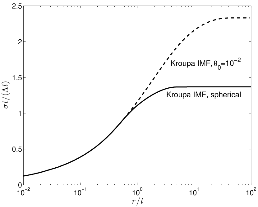
Figure 1.— Line-width $\sigma(r)$ versus size, normalized to the characteristic values in §  2, for outflows driven by stars drawn from the Kroupa (2001) IMF. If outflows are spherical, the theory of § 4.1.1 gives the lower curve; if they are collimated, the theory of § 4.1.2 gives the upper curve. At scales much smaller than the driving scale ${\ell}$, $\sigma\propto r^{1/2}$ – in agreement with the Larson’s-law scalings for molecular clouds (Larson 1981) as reported by Solomon et al. (1987).

Table 1Turbulence enhancement factors.

Mass function	${\cal E}$ (isotropic)	${\cal E}$ ($\theta_{0}=10^{-2}$)
Single-mass	1.0	3.04
Kroupa (2001) IMF	1.85	5.38

The influence of collimation on $\sigma(r)$ is illustrated in figure 1, which displays numerical integrations of equation (20). Two points can be drawn from these results: (1) A finite thermal sound speed is of no practical consequence so long as ${\ell}>c_{s}{t}$, since solutions converge when $\sigma>c_{s}$; (2) $\sigma(r)$ continues to rise until $r\simeq\max{({r_{m1}})}$. (Recall that $\max({r_{m1}})$ refers to the value obtained by setting ${\cal I}\to\max{\cal I}$.) However the rise in $\sigma(r)$ slows to zero as this limit is approached.

We expect the coupling coefficient $\Lambda$ to depend somewhat on the degree of collimation, thanks to complicated phenomena like collisions between young outflows (Cunningham et al. 2006), although the sense and magnitude of this dependence are unknown.

4.2. Finite-size regions

What if the region of interest (a dense “clump”, say) is too small to catch all the outflow momentum? The eruption of outflows from protocluster regions is frequently observed, and this process deserves special attention. Matzner & McKee (2000) calculated the mass ejection rate in this case; we wish to consider the outflows’ dynamical effects.

It is not sufficient to simply evaluate $\sigma(r)$ at the clump size $R$ using the results of the previous section. Equation (20) assumes a homogeneous background on scales larger than $r$, as $\sigma(r)$ reflects the downward cascade driven by outflows merging on larger scales, as well as the upward cascade composed by those outflows as they expand. However, outflows take momentum as well as mass with them when they escape. Collimation allows this to happen in some directions without the entire clump being unbound. Specifically, escape occurs in direction $\mu$ when $\hat{\cal I}(|\mu|)>{\cal I}_{\rm esc}$, where

$${\cal I}_{\rm esc}=c_{g}Mv_{\rm esc}$$ (31)

if $M=M(R)$ and $v_{\rm esc}=(2GM/R)^{1/2}$ are the mass and escape velocity of the region. The factor $c_{g}$ accounts for gravitational deceleration of an expanding shell, which saps its momentum. It is close to unity, however: for density distributions $\rho(r)\propto r^{-k_{\rho}}$, Matzner & McKee (2000) found

$$c_{g}=\left(9-3k_{\rho}\over 8-3k_{\rho}\right)^{1/2}$$ (32)

(their equation [A13]). This formula holds when outflows are driven impulsively – a safe assumption, so long as the wind that drives an outflow has a duration similar to the free-fall time of its collapsing, overdense core.

Given that outflow intensities exceeding ${\cal I}_{\rm esc}$ get away, the theory of § 4.1 is easy to modify: simply replace ${\cal S}_{\rm tot}$ with ${\cal S}({\cal I}_{\rm esc})$, throwing away the remaining momentum. It is important to realize that some outflows emerge from the clump surface and rain back on it later; the replacement just suggested treats them no differently from those that merge within the clump. Although approximate, this approach captures the essential division between capture and escape.

The effect of outflow eruptions on the velocity scale $\sigma(R)$ is determined by how much outflow momentum is eliminated in this procedure. It depends, therefore, on the dimensionless ratio ${{\cal I}_{\rm esc}/\bar{\cal I}}$ as well as on the shape of ${\cal S}({\cal I})$ (see also § 2.1). This dependence is illustrated in figure 2, where a slow dependence on ${\cal I}_{\rm esc}/\bar{\cal I}$ is apparent. This is natural, because the apparent intensity $\hat{\cal I}$ can exceed $\bar{\cal I}$ by a factor of $10^{6.7}$ in the model plotted – of which $10^{2.7}$ comes from the range of stellar masses, and $10^{4}$ arises from collimation. For a default model in which we adopt the Kroupa (2001) IMF, take ${v_{c}}$ to be independent of ${M_{\star}}$, consider winds to be collimated with $\theta_{0}=10^{-2}$, and take $a_{\rm ext}=0$, we find

$${\sigma^{2}{t}^{2}\over{\ell}^{2}}\simeq{c_{s}^{2}{t}^{2}\over{\ell}^{2}}+\Lambda^{2}\left[K_{1}^{-2\eta}+K_{2}^{-2\eta}\left(r\over{\ell}\right)^{-\eta}\right]^{-1/\eta}$$ (33)

where the fit parameters $K_{1}$, $K_{2}$, and $\eta$ are functions of ${{\cal I}_{\rm esc}/\bar{\cal I}}$:

$$K_{1}=\left[2.33^{-10}+\left(0.32+0.40\log_{10}{{\cal I}_{\rm esc}\over\bar{\cal I}}\right)^{-10}\right]^{-1/10},$$ (34)

$$K_{2}=\left[1.22^{-6}+\left(0.55+0.26\log_{10}{{\cal I}_{\rm esc}\over\bar{\cal I}}\right)^{-6}\right]^{-1/6},$$ (35)

and

$$\eta={11+15\log_{10}({\cal I}_{\rm esc}/\bar{\cal I})\over 1+10\log_{10}({\cal I}_{\rm esc}/\bar{\cal I})}.$$ (36)

This fit reproduces the numerical evaluation of $\sigma(r)$ to within 5% for ${\cal I}_{\rm esc}>6{\cal I}$. The quantities used in these formulae are, in convenient form,

$${{\cal I}_{\rm esc}\over\bar{\cal I}}=770\,M_{3}^{5/4}\Sigma_{\rm cgs}^{1/4}{40\,\rm km\,s^{-1}\over{v_{c}}},$$ (37)

$${\ell}=0.079\,M_{3}^{5/28}\Sigma_{\rm cgs}^{-15/28}\left({40\,\rm km\,s^{-1}\over{v_{c}}}{0.034\over{\mbox{SFR}_{\rm ff}}}\right)^{1/7}\,\rm pc,$$ (38)

and

$${{\ell}\over{t}}=1.24\,M_{3}^{-1/28}\Sigma_{\rm cgs}^{3/28}\left({{v_{c}}\over 40\,\rm km\,s^{-1}}\right)^{4/7}\left({0.034\over{\mbox{SFR}_{\rm ff}}}\right)^{3/7}\,{\rm km\over s}$$ (39)

where $M(R)=10^{3}M_{3}\,M_{\odot}$ and $M(R)/(\pi R^{2})=\Sigma_{\rm cgs}$ g cm^-2, and we used $k_{\rho}=1.5$ to evaluate $c_{g}$.

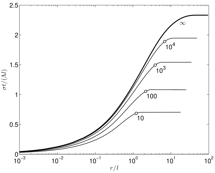
Figure 2.— Effect of finite clump radius on turbulence driven by collimated outflows ($\theta_{0}=10^{-2}$) driven by stars drawn from the Kroupa (2001) IMF. The thick curve represents an infinite uniform medium; the other curves are labeled by ${\cal I}_{\rm esc}/\bar{\cal I}$, which determines how much momentum is lost from a finite clump. Circles mark the edge of the region for fiducial parameters $n_{H4}=1$, ${v_{c}}=40$ km s^-1, ${\mbox{SFR}_{\rm ff}}=0.034$, and $\Lambda=1$.

5. Comparison to simulation

The simulation by Li & Nakamura (2006) offers the closest comparison to the theory presented above. These authors simulate a self-gravitating, weakly magnetized, initially turbulent cloud, identifying regions of localized collapse and replacing them with spherical outflows. Using their fiducial conversion from code units to physical units, their outflow momentum scale is nearly constant at ${\cal I}=10^{39.7}\rm g\,cm\,s^{-1}$. The 960 $M_{\odot}$ of cloud gas is initially arranged in a mildly centrally peaked density profile of outer radius 0.75 pc, and becomes more centrally condensed over the course of the run. After 0.6 Myr star formation begins in earnest, and between 0.9 and 1.2 Myr the stellar fraction increases from 6.5% to 13.4% of the cloud mass. Li & Nakamura report a final, three-dimensional rms velocity of 1.5 km s^-1 corresponding to $\sigma=0.85\rm\,km\,s^{-1}$.

If one assumes that the gas has contracted by a fraction $f_{R}$ of its initial radius during the period 0.9-1.2 Myr, then $\rho_{0}\simeq 10^{-19.4}f_{R}^{-3}\,\rm g\,cm^{-3}$ and ${\cal S}\simeq 10^{-66.6}f_{R}^{-3}\,\rm cm^{-3}\,s^{-1}$ in that period. Equation (17) then predicts $\sigma=1.7f_{R}\Lambda\rm\,km\,s^{-1}$, which is consistent with the Li & Nakamura results if $\Lambda=0.6f_{R}^{-3/7}$. Contraction by $f_{R}=1/2$ appears reasonable based on their figure 2, in which case

$$\Lambda\simeq 0.8.$$

This seems entirely consistent with our expectations from § 2 that $\Lambda\sim 1$. Note, however, that one should expect changes in numerical resolution, cloud magnetization, and outflow collimation to be accompanied by variations in $\Lambda$.

Li & Nakamura also mention that collimated outflows appear to drive more vigorous turbulence, as we would expect from § 4.1.2. Nakamura & Li (2006) have modified their previous simulations by collimating outflows within 30^∘ half opening angle, and report that the enhancement is not discernible from the simulations. In our theory, this modification amounts to increasing ${\cal I}$ by a factor of 7.5 while holding ${\cal S}{\cal I}$ fixed; we would expect $\sigma$ to increase by $7.5^{1/7}=1.3$ (as in eq. [2]), so long as $\Lambda$ does not change. Whether this mild enhancement of turbulent velocity is seen in simulation will require further investigation. In an equilibrium cloud, as our referee points out, one must tease this effect from the redistribution of mass caused by more vigorous turbulence.

A deeper investigation of the same class of model is reported by Nakamura & Li (2007), who report several results in line with our predictions. In this work, outflows posses a 30^∘ “jet” component and a uniform “wind” component. The authors report that the jet component is more effective at driving turbulence, based on the slowdown of star formation observed if jets are strengthened (all else being equal). Their turbulent power spectrum obeys $E(k)\propto k^{-2}$ as anticipated in equation (10), and flattens at large scales – possibly reflecting the flattening of $\sigma(r)$ (figure 1). Finally, they obtain an equilibrium density profile $\rho\propto r^{-1.5}$, in line with the argument we present below in §7.

Mac Low (2000) has also simulated turbulence driven by collimated sources, but a direct comparison is not possible because the driving field in his simulation was steady rather than impulsive.

6. Comparison to observation: NGC 1333

Located within the Perseus molecular cloud, the NGC 1333 reflection nebula is the site of a vigorous burst of clustered star formation within a dense molecular clump. The current population of at least 143 young stars is estimated to be 1-2 Myr old (Lada et al. 1996), and about ten molecular outflows and Herbig-Haro systems emerge from the most recently formed objects. Lada & Lada (2003) estimate a stellar mass of $\sim 79\,M_{\odot}$, based on the limiting $K$ magnitude of $14.5$. Distance estimates range from $D=$210 pc to 350 pc, as discussed by Warin et al. (1996).

Ridge et al. (2003) map the NGC 1333 core (and many others) in ¹³CO(1-0), C¹⁸O(1-0), and C¹⁸O(2-1), probing sequentially smaller and denser regions. They derive masses from a large velocity gradient analysis; combining these with their reported velocity dispersions, and assuming that gas dominates the mass budget, we derive the virial parameter (Bertoldi & McKee 1992)

$$\alpha_{\rm vir}\equiv{5R\sigma(R)^{2}\over GM(R)}=\left(1.27,1.32,1.19\right){220\,\rm pc\over D}$$ (40)

for ¹³CO(1-0), C¹⁸O(1-0), and C¹⁸O(2-1), respectively. Since $\alpha_{\rm vir}$ is thought to vary, in strongly self-gravitating regions, between 1.11 (for molecular clouds; Solomon et al. 1987) and 1.34 (for massive, magnetized molecular cores; McKee & Tan 2003), we adopt $D=220$ pc (close to $D=212$ pc adopted by Quillen et al. 2005). The embedded star cluster then have an effective radius $R=0.39$ pc, scaling the value given by Lada & Lada (2003) to the closer distance; the enclosed mass is then 446 $M_{\odot}$, and the escape velocity is 3.1 km s^-1. The velocity dispersion at the same radius is $\sigma=1.1\,\rm km\,s^{-1}$.

Can this velocity dispersion be maintained by the protocluster outflows? To evaluate the formulae in § 4.1 and §4.2, we adopt the Kroupa (2001) IMF and assume the current star formation rate equals 79 $M_{\odot}$ per Myr. Other model parameters are ${\cal S}_{\rm tot}=10^{-65.8}\rm cm^{-3}\,s^{-1}$, $\rho_{0}=10^{-18.9}\rm g\,cm^{-3}$, $T=20$ K, $\theta_{0}=10^{-2}$, and ${\cal I}_{\rm esc}=10^{41.5}$ g cm s^-1 (where we have used $k_{\rho}=1.35$ to estimate $c_{g}=1.1$ in eq. [32]). For reference, these values give ${\mbox{SFR}_{\rm ff}}\simeq 0.034$ in the region of interest – virtually identical to the value ${\mbox{SFR}_{\rm ff}}=0.038$ we derive from the Krumholz & McKee (2005) theory. We take $a_{\rm ext}=0$ to probe the influence of outflows alone.

Using ${v_{c}}=40$ km s^-1 and applying the prescription of §4.2 to predict the velocity dispersion at $R=0.39$ pc, we find $\sigma(R)=1.12(\Lambda/0.8)$ km s^-1. This is entirely consistent with the observed value of 1.1 km s^-1, for precisely the same value of $\Lambda$ we estimated in § 5. This result is entirely consistent with the proposition that turbulence in the star-forming region of NGC 1333 has been regenerated by outflows. The cluster outflow inferred by Warin et al. (1996) could then legitimately be viewed as the mass ejected by erupting jets, and the inflow detected by Walsh et al. (2006) might represent a return flow of gas ejected below the escape speed.

Although the value ${v_{c}}=40$ km s^-1 (which was justified in § 3 using the observational relations reported by Richer et al. 2000) is in line with the momentum of the NGC 1333 outflow HH 7-11 as estimated by Snell & Edwards (1981), Knee & Sandell (2000) and Quillen et al. (2005) have inferred significantly lower momenta for the NGC 1333 outflows. Knee & Sandell estimate $\sim 1M_{\odot}$ km s^-1 per outflow for ten currently active outflows, and Quillen et al. derive a similar momentum scale for the explosions that open cavities in the gas. Given that the mean stellar mass in the Kroupa (2001) IMF is $0.21\,M_{\odot}$, this momentum scale corresponds to $v_{c}\sim 5$ km s^-1. In the formalism of § 4.2, this lower value would imply $\sigma(R)=0.47\Lambda$ km s^-1.

It is possible that, for strongly collimated outflows in a real, magnetized star-forming region like NGC 1333, $\Lambda=2.3$ as required to make this lower estimate consistent with the observed value of 1.1 km s^-1. However it is equally probable that the inference ${v_{c}}\sim 5$ km s^-1 is an underestimate: compare this to the estimates in § 3, and note that the minimum value estimated by Richer et al. (2000, in their § III.B) is $\sim$30 km s^-1. One solution to this discrepancy could be that the outflows now observed in NGC 1333 are simply smaller than the average – possible, since the median value of $M_{\star}$ in the Kroupa (2001) IMF is 2.6 times lower than the mean value. Alternatively these outflows could be more powerful than Knee & Sandell (2000) report. The fact that they find a $2.5\,M_{\odot}$ km s^-1 as the net momentum of HH 7-11 in their ¹²CO(3-2) and ¹²CO(2-1) survey, whereas Snell & Edwards (1981) find $\sim 34$ km s^-1 for the same outflow in observations involving the four transitions ^12,13CO(J=2-1,1-0), raises this possibility. CO optical depth, uncorrected inclination, motions at velocities close to systemic, and loss of momentum from the cloud can all cause outflow momentum to be underestimated. (See Walawender et al. 2005 for a discussion of some problems in the determination of outflow momentum.) Moreover, the most noticeable outflows are the young, rapidly expanding ones. Since these are still being driven, they will not have acquired their final momenta. Finally, note that very little mass can be ejected from the region by outflows if ${v_{c}}$ is as low as 5 km s^-1: the theory of Matzner & McKee (2000) predicts a star formation efficiency $\varepsilon\simeq 88\%$ in this case, whereas $\varepsilon\simeq 47\%$ if ${v_{c}}=40$ km s^-1. The latter value is more consistent with the fact that only $\sim 18\%$ of the mass is currently in stars.

For all of these reasons we consider it most likely that turbulence in NGC 1333 is driven by outflows with ${v_{c}}\sim 40$ km s^-1 (such that $\Lambda\simeq 0.8$ in the theory of §  4.2), although the alternatives – that $\Lambda\simeq 2.3$, or that outflows are only a minor contributor to the turbulence – cannot be ruled out. The last option is especially unattractive, as it leaves unanswered the question of how turbulent energy is regenerated there.

7. Implications for star cluster formation

Our analysis of NGC 1333 supports the assertion that outflow-driven turbulence affects the dynamical state of gas clumps while star clusters form within them. How, then, does feedback influence the creation of star clusters?

A preliminary answer can be gleaned from figure 3, where we calculate $\alpha_{\rm vir}$ for cluster-forming regions of various total mass ($M$) and column density ($\Sigma=M/(\pi R^{2})$) using the formalism of § 4.2. In this calculation the region was assumed to be neither expanding nor contracting, and devoid of any additional source of turbulence ($a_{\rm ext}=0$); outflows were collimated with $\theta_{0}=10^{-2}$ and ${v_{c}}=40$ km s^-1, and the Kroupa (2001) IMF was adopted. In the left panel, the star formation rate parameter ${\mbox{SFR}_{\rm ff}}$ was held fixed at the value 0.034 we derived for NGC 1333; on the right, ${\mbox{SFR}_{\rm ff}}$ and $\alpha_{\rm vir}$ were derived self-consistently according to the model of Krumholz & McKee (2005); however the gas temperature was held fixed at 20 K for simplicity.

We expect that there exists a critical value of $\alpha_{\rm vir}$, between 1 and 2, such that a cluster-forming clump will be in virial equilibrium given a moderate external pressure; for instance, McKee & Tan (2003) derive $\alpha_{\rm vir}=1.34$ for their equilibrium model of magnetized, turbulent cores. Smaller values of $\alpha_{\rm vir}$ imply contraction. Higher values imply either expansion, or require a strong confining pressure.

An immediate conclusion from figure 3 is the existence of an outflow-driven equilibrium state ($\alpha_{\rm vir}\simeq 1.5$) for column densities and masses relevant to star cluster formation. It is however an unstable equilibrium: since $\partial\alpha_{\rm vir}/\partial\Sigma<0$ at fixed mass, turbulent support is weakened if an equilibrium clump is compressed. The instability is reduced – though not removed – by the self-regulation of the star formation rate in the Krumholz & McKee (2005) model. It would be reduced even further if we were to account for heating of the gas by star formation, as the sound speed enters (weakly) into the Krumholz & McKee theory.

Unstable equilibria were previously found by McKee (1989) in models for giant molecular clouds, and by Matzner (1999) and Matzner & McKee (1999b) in simpler models for star cluster formation. In fact, instability is generic to any model in which ${\mbox{SFR}_{\rm ff}}$ and ${v_{c}}$ are slowly varying functions of the cloud parameters. For a virialized cloud this can be seen by comparing the cloud dissipation rate $\sim\sigma(R)^{5}/G$ with its energy input rate – which scales as the star formation rate $\sim{\mbox{SFR}_{\rm ff}}\sigma(R)^{3}/G$, times the energy injection per unit star mass $\sim{v_{c}}\sigma(R)$. So long as ${\mbox{SFR}_{\rm ff}}{v_{c}}$ does not increase as fast as $\sigma^{2}$ when the cloud contracts, dissipation overcomes energy injection. Sharp thresholds, such as the photoionization column in McKee (1989), are therefore required for stable equilibria.

The scenario for star cluster formation implied by figure 3 is qualitatively consistent with the one advanced by Tan et al. (2006) and Krumholz & Tan (2006), in that turbulence supplied by outflows is important enough to slow collapse over several, perhaps many, crossing times. Because the equilibrium state is unstable, is also consistent with proposal by Li & Nakamura (2006) that this support may fail in some circumstances, and that this might lead to a state of collapse that triggers massive star formation. However, massive-star outflows are almost certainly more powerful than our simple model has assumed – as discussed in § 3 and by Tan & McKee (2002). If there is a column density threshold for massive star formation, then it is possible that the feedback from these stars creates a stable equilibrium – in which $\Sigma$ remains near the threshold. Alternatively, massive stars might disrupt the clump outright; we leave these questions for future investigation.

The form of the line-width-size relation $\sigma(r)$ affects the internal structure and dynamics of a clump, in addition to its global expansion or contraction. Suppose we define $\beta(r)=d\ln\sigma/d\ln r$ as the logarithmic slope of this relation. In a singular polytropic model for the clump (McKee & Tan 2003), the density index $k_{\rho}$ (in $\rho\propto r^{-k_{\rho}}$) is related to $\beta$ through $k_{\rho}=2-2\beta$ (and both $\beta$ and $k_{\rho}$ are assumed constant in radius). In our model, $\beta(R)$ can take any value between 0 and 1/2, depending on the ratio between $R$ and the turnover in $\sigma(r)$ – as seen in figure 2. This figure also shows that star-forming regions with $n_{H}\sim 10^{4}$ cm^-3 have radii near this turnover, so that $\beta(R)\simeq 1/4$ – generally consistent with the value $\beta=0.21\pm 0.03$ obtained for massive cores and clumps by Caselli & Myers (1995). More specifically, the fit given in equation (33) implies

$$\beta\simeq\frac{1}{2H\left(1+{c_{s}^{2}{t}^{2}\over\Lambda^{2}R{\ell}}H\right)}$$ (41)

where

$$H=1+\left(\frac{K_{2}}{K_{1}}\right)^{2\eta}\left(\frac{R}{{\ell}}\right)^{\eta}.$$ (42)

To the extent that the McKee & Tan (2003) model can be generalized to our model for turbulence, $\beta\simeq 1/4$ implies $k_{\rho}\simeq 1.5$ on the scale of the region. This estimate coincides with the value McKee & Tan (2003) adopted after a survey of the observational literature. If our proposal for the origin of $k_{\rho}$ is correct, then one would expect that $k_{\rho}$ is steeper (closer to 2) in denser and more massive regions (so long as turbulence is dominated by outflows), as both $R/{\ell}$ is higher there, and as ${\cal I}/{\cal I}_{\rm esc}$ is lower. Note that Huff & Stahler (2006) derive $k_{\rho}\simeq 2$ for the birth region of the Orion Nebula Cluster.

The line-width-size index $\beta$ also enters into estimates for the typical radii of protostellar disks. Kratter & Matzner (2006) calculate the specific angular momenta of cores prior to their collapse, and find that a larger value of $\beta$ leads to a greater angular momentum. Note that, since $\beta$ is a decreasing function of $r$, its value is greater on the core scale than on the clump scale. Tan et al. (2006) have previously proposed that $\beta\simeq 1/2$ on small scales, falling to $\sim 1/4$ on scales large enough to sample the tidal field. We propose that this shift is produced by the dynamics of driving – and shapes the gravitational potential, rather than reflecting it.

8. Caveats

The theory presented here relies on several assumptions and approximations. The central hypothesis, as stated in §4, is that a strongly dissipative, supersonic turbulence can be described as a cascade of (scalar) momentum to small scales in much the same way that Kolmogorov turbulence can be described as an energy cascade. This is not too bold, as it agrees with the spectral slopes observed in simulations of these cascades. In § 4.1 we assumed that these cascades will simply add, in the case that turbulence is driven by more than one type of source. In § 4.1.2 we assumed, further, that this superposition can be applied to collimated outflows – if the variation of strength with angle is treated in the same manner as a population of isotropic sources of different strengths. Moreover, our treatment in § 4.2 assumes that the turbulent velocity in a region of finite radius can be estimated by (1) discarding momentum ejected in escaping outflows and (2) evaluating the resulting line-width-size relation at the scale of the region. Finally, we have assumed that the differences between outflow-driven turbulence in magnetized and unmagnetized gas can be encompassed by modifying the coupling coefficient $\Lambda$, and in § 7, by a modifying the critical virial parameter corresponding to collapse. All of these assumptions are sure to be approximate at some level, and must be tested against numerical simulations and observations more thoroughly than we have done in § 5 and § 6.

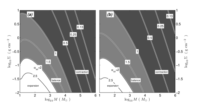
Figure 3.— Virial parameter $\alpha_{\rm vir}$ for outflow-driven turbulence within clouds of various total mass $M$ and column density $\Sigma=M/(\pi R^{2})$. Outflows are assumed to be collimated ($\theta_{0}=10^{-2}$) and driven, with ${v_{c}}=40$ km s^-1, by stars drawn from the Kroupa (2001) IMF; $\Lambda=1$. In (a), ${\mbox{SFR}_{\rm ff}}$ is held constant at 0.034; in (b), ${\mbox{SFR}_{\rm ff}}$ is derived self-consistently from $\alpha_{\rm vir}$ using the star formation rate model of Krumholz & McKee (2005). In both cases the gas temperature is assumed to be 20 K throughout, and there is no external driving ($a_{\rm ext}=0$). Conditions for expansion and contraction are estimated assuming that virial balance corresponds to a value of $\alpha_{\rm vir}$ between 1 and 2.

9. Summary and Conclusions

Based on our observation that the spectral slope of supersonic turbulence implies a momentum cascade rather than an energy cascade, we have constructed a simple model for turbulence stirred by momentum injection from stellar outflows. A key feature of our model is that turbulence is enhanced if momentum injection is spread amongst outflows of a wide range of strengths, or, by extension, if outflows are strongly collimated. These effects allow for some of the momentum to be deposited on relatively large scales where turbulent decay is slow. The diversity of outflow strengths (reflecting the range of stellar masses), and their strong collimation by magnetic fields, both imply that real outflows are quite effective at driving turbulence.

Our comparison to NGC 1333 supports the assertion that turbulence in the cluster-forming gas has been entirely regenerated by outflows. Although uncertainties regarding the outflow momentum scale and the value of the theoretical outflow-turbulence coupling coefficient $\Lambda$ limit the strength of this conclusion, these uncertainties will be eliminated by future numerical and observational studies.

In our fiducial model, outflows will maintain turbulence within cluster-forming regions of a few thousand solar masses, whose column densities are $\sim 0.3-1$ g cm^-2. Intriguingly, the energetic equilibrium in these models is an unstable one. It is possible that this leads to global contraction or collapse, as Li & Nakamura (2006) have suggested. However this instability could equally be an artifact of our assumption that outflow momentum scales in proportion to the mass of the forming star.

The structure of a turbulence-supported region reflects its turbulent spectral slope. The radial density index takes values close to -2 if turbulence is driven on small scales, or close to -1 if it is driven on scales larger than the region of interest. Our model predicts intermediate slopes ($\sim-1.5$) because outflow collimation allows both of these to occur simultaneously. We expect this slope, which is consistent with observations of cluster-forming regions, to steepen in regions that catch outflow momentum more effectively.

Although our model was developed to address protostellar outflows, it could in principle be extended to other forms of driven, supersonic turbulence in radiative gas, such as HII-region-driven turbulence in molecular clouds (Matzner 2002) or supernova-driven turbulence in the diffuse interstellar medium (Mac Low et al. 2001).

References

- Adams & Laughlin (2001) Adams, F. C. & Laughlin, G. 2001, Icarus, 150, 151
- Bertoldi & McKee (1992) Bertoldi, F. & McKee, C. F. 1992, ApJ, 395, 140
- Blaauw & Morgan (1954) Blaauw, A. & Morgan, W. W. 1954, ApJ, 119, 625
- Brown et al. (2005) Brown, M. E., Trujillo, C. A., & Rabinowitz, D. L. 2005, ApJ, 635, L97
- Caselli & Myers (1995) Caselli, P. & Myers, P. C. 1995, ApJ, 446, 665
- Cunningham et al. (2006) Cunningham, A. J., Frank, A., & Blackman, E. G. 2006, ApJ, 646, 1059
- Huff & Stahler (2006) Huff, E. M. & Stahler, S. W. 2006, ApJ, 644, 355
- Kida (1979) Kida, S. 1979, Journal of Fluid Mechanics, 93, 337
- Knee & Sandell (2000) Knee, L. B. G. & Sandell, G. 2000, A&A, 361, 671
- Kratter & Matzner (2006) Kratter, K. M. & Matzner, C. D. 2006, MNRAS, in press (ArXiv e-print astro-ph/0609692)
- Kroupa (2001) Kroupa, P. 2001, MNRAS, 322, 231
- Krumholz et al. (2006) Krumholz, M. R., Matzner, C. D., & McKee, C. F. 2006, ApJ, in press (ArXiv e-print astro-ph/0608471)
- Krumholz & McKee (2005) Krumholz, M. R. & McKee, C. F. 2005, ApJ, 630, 250
- Krumholz & Tan (2006) Krumholz, M. R. & Tan, J. C. 2006, ArXiv e-print astro-ph/0606277
- Lada et al. (1996) Lada, C. J., Alves, J., & Lada, E. A. 1996, AJ, 111, 1964
- Lada & Lada (2003) Lada, C. J. & Lada, E. A. 2003, ARA&A, 41, 57
- Larson (1981) Larson, R. B. 1981, MNRAS, 194, 809
- Li & Nakamura (2006) Li, Z.-Y. & Nakamura, F. 2006, ApJ, 640, L187
- Mac Low (1999) Mac Low, M.-M. 1999, ApJ, 524, 169
- Mac Low (2000) Mac Low, M.-M. 2000, in Star formation from the small to the large scale. ESLAB symposium 33 Noordwijk, The Netherlands. Edited by F. Favata, A. Kaas, and A. Wilson., 457
- Mac Low et al. (2001) Mac Low, M.-M., Balsara, D., Avillez, M. A., & Kim, J. 2001, submitted to ApJ
- Mac Low et al. (1998) Mac Low, M.-M., Klessen, R. S., Burkert, A., & Smith, M. D. 1998, Physical Review Letters, 80, 2754
- Matzner (1999) Matzner, C. D. 1999, PhD thesis, U. C. Berkeley
- Matzner (2002) —. 2002, ApJ, 566, 302
- Matzner & McKee (1999a) Matzner, C. D. & McKee, C. F. 1999a, ApJ, 526, L109
- Matzner & McKee (1999b) Matzner, C. D. & McKee, C. F. 1999b, in Star Formation 1999, ed. T. Nakamoto, Nobeyama Radio Observatory, 353–357
- Matzner & McKee (2000) —. 2000, ApJ, 545, 364
- McKee (1989) McKee, C. F. 1989, ApJ, 345, 782
- McKee & Tan (2003) McKee, C. F. & Tan, J. C. 2003, ApJ, 585, 850
- McKee & Williams (1997) McKee, C. F. & Williams, J. P. 1997, ApJ, 476, 144
- McKee et al. (1993) McKee, C. F., Zweibel, E. G., Goodman, A. A., & Heiles, C. 1993, in Protostars and Planets IV,/cdfghlnstwy, 327
- Nakamura & Li (2006) Nakamura, F. & Li, Z.-Y. 2006, in IAU Symposium, Vol. 640, in prep
- Nakamura & Li (2007) Nakamura, F. & Li, Z.-Y. 2007, ApJ, submitted
- Norman & Silk (1980) Norman, C. & Silk, J. 1980, ApJ, 238, 158
- Padoan & Nordlund (2002) Padoan, P. & Nordlund, Å. 2002, ApJ, 576, 870
- Palla et al. (2005) Palla, F., Randich, S., Flaccomio, E., & Pallavicini, R. 2005, ApJ, 626, L49
- Palla & Stahler (1992) Palla, F. & Stahler, S. W. 1992, ApJ, 392, 667
- Palla & Stahler (1999) —. 1999, ApJ, 525, 772
- Porter et al. (1992) Porter, D. H., Pouquet, A., & Woodward, P. R. 1992, Physical Review Letters, 68, 3156
- Quillen et al. (2005) Quillen, A. C., Thorndike, S. L., Cunningham, A., Frank, A., Gutermuth, R. A., Blackman, E. G., Pipher, J. L., & Ridge, N. 2005, ApJ, 632, 941
- Richer et al. (2000) Richer, J. S., Shepherd, D. S., Cabrit, S., Bachiller, R., & Churchwell, E. 2000, in Protostars and Planets IV (Tucson: University of Arizona Press; eds Mannings, V., Boss, A.P., Russell, S. S.), 867
- Ridge et al. (2003) Ridge, N. A., Wilson, T. L., Megeath, S. T., Allen, L. E., & Myers, P. C. 2003, AJ, 126, 286
- Snell & Edwards (1981) Snell, R. L. & Edwards, S. 1981, ApJ, 251, 103
- Solomon et al. (1987) Solomon, P. M., Rivolo, A. R., Barrett, J., & Yahil, A. 1987, ApJ, 319, 730
- Stone et al. (1998) Stone, J. M., Ostriker, E. C., & Gammie, C. F. 1998, ApJ, 508, L99
- Tan & McKee (2000) Tan, J. & McKee, C. F. 2000, in Starbursts: Near and Far
- Tan et al. (2006) Tan, J. C., Krumholz, M. R., & McKee, C. F. 2006, ApJ, 641, L121
- Tan & McKee (2002) Tan, J. C. & McKee, C. F. 2002, in ASP Conf. Ser. 267: Hot Star Workshop III: The Earliest Phases of Massive Star Birth, ed. P. Crowther, 267–+
- Walawender et al. (2005) Walawender, J., Bally, J., & Reipurth, B. 2005, AJ, 129, 2308
- Walsh et al. (2006) Walsh, A. J., Bourke, T. L., & Myers, P. C. 2006, ApJ, 637, 860
- Warin et al. (1996) Warin, S., Castets, A., Langer, W., Wilson, R., & Pagani, L. 1996, A&A, 306, 935