Observations of the High Redshift Universe

ABSTRACT

In this series of lectures, aimed for non-specialists, I review the considerable progress that has been made in the past decade in understanding how galaxies form and evolve. Complementing the presentations of my theoretical colleagues, I focus primarily on the impressive achievements of observational astronomers. A credible framework, the $\Lambda$CDM model, now exists for interpreting these observations: this is a universe with dominant dark energy whose structure grows slowly from the gravitational clumping of dark matter halos in which baryonic gas cools and forms stars. The standard model fares well in matching the detailed properties of local galaxies, and is addressing the growing body of detailed multi-wavelength data at high redshift. Both the star formation history and the assembly of stellar mass can now be empirically traced from redshifts $z\simeq$6 to the present day, but how the various distant populations relate to one another and precisely how stellar assembly is regulated by feedback and environmental processes remains unclear. In the latter part of my lectures, I discuss how these studies are being extended to locate and characterize the earliest sources beyond $z\simeq$6. Did early star-forming galaxies contribute significantly to the reionization process and over what period did this occur? Neither theory nor observations are well-developed in this frontier topic but the first results are exciting and provide important guidance on how we might use more powerful future facilities to fill in the details.

1 Role of Observations in Cosmology & Galaxy Formation

1.1 The Observational Renaissance

These are exciting times in the field of cosmology and galaxy formation! To justify this claim it is useful to review the dramatic progress made in the subject over the past $\simeq$25 years. I remember vividly the first distant galaxy conference I attended: the IAU Symposium 92 Objects of High Redshift, held in Los Angeles in 1979. Although the motivation was strong and many observers were pushing their 4 meter telescopes to new limits, most imaging detectors were still photographic plates with efficiencies of a few percent and there was no significant population of sources beyond a redshift of $z$=0.5, other than some radio galaxies to $z\simeq$1 and more distant quasars.

In fact, the present landscape in the subject would have been barely recognizable even in 1990. In the cosmological arena, convincing angular fluctuations had not yet been detected in the cosmic microwave background nor was there any consensus on the total energy density $\Omega_{TOT}$. Although the role of dark matter in galaxy formation was fairly well appreciated, neither its amount nor its power spectrum were particularly well-constrained. The presence of dark energy had not been uncovered and controversy still reigned over one of the most basic parameters of the Universe: the current expansion rate as measured by Hubble’s constant. In galaxy formation, although evolution was frequently claimed in the counts and colors of galaxies, the physical interpretation was confused. In particular, there was little synergy between observations of faint galaxies and models of structure formation.

In the present series of lectures, aimed for non-specialists, I hope to show that we stand at a truly remarkable time in the history of our subject, largely (but clearly not exclusively) by virtue of a growth in observational capabilities. By the standards of all but the most accurate laboratory physicist, we have ‘precise’ measures of the form and energy content of our Universe and a detailed physical understanding of how structures grow and evolve. We have successfully charted and studied the distribution and properties of hundreds of thousands of nearby galaxies in controlled surveys and probed their luminous precursors out to redshift $z\simeq$6 - corresponding to a period only 1 Gyr after the Big Bang. Most importantly, a standard model has emerged which, through detailed numerical simulations, is capable of detailed predictions and interpretation of observables. Many puzzles remain, as we will see, but the progress is truly impressive.

This gives us confidence to begin addressing the final frontier in galaxy evolution: the earliest stellar systems and their influence on the intergalactic medium. When did the first substantial stellar systems begin to shine? Were they responsible for reionizing hydrogen in intergalactic space and what physical processes occurring during these early times influenced the subsequent evolution of normal galaxies?

Let’s begin by considering a crude measure of our recent progress. Figure 1 shows the rapid pace of discovery in terms of the relative fraction of the refereed astronomical literature in two North American journals pertaining to studies of galaxy evolution and cosmology. These are cast alongside some milestones in the history of optical facilities and the provision of widely-used datasets. The figure raises the interesting question of whether more publications in a given field means most of the key questions are being answered. Certainly, we can conclude that more researchers are being drawn to work in the area. But some might argue that new students should move into other, less well-developed, fields. Indeed, the progress in cosmology, in particular, is so rapid that some have raised the specter that the subject may soon reaching some form of natural conclusion (c.f. Horgan 1998).

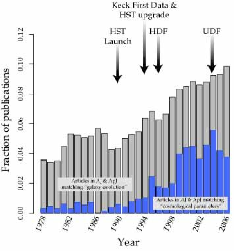
Figure 1: Fraction of the refereed astronomical literature in two North American journals related to galaxy evolution and the cosmological parameters. The survey implies more than a doubling in fractional share over the past 15 years. Some possibly-associated milestones in the provision of unique facilities and datasets are marked (courtesy: J. Brinchmann).

I believe, however, that the rapid growth in the share of publications is largely a reflection of new-found observational capabilities. We are witnessing an expansion of exploration which will most likely be followed with a more detailed physical phase where we will be concerned with understanding how galaxies form and evolve.

1.2 Observations Lead to Surprises

It’s worth emphasizing that many of the key features which define our current view of the Universe were either not anticipated by theory or initially rejected as unreasonable. Here is my personal short list of surprising observations which have shaped our view of the cosmos:

1. The cosmic expansion discovered by Slipher and Hubble during the period 1917-1925 was not anticipated and took many years to be accepted. Despite the observational evidence and the prediction from General Relativity for evolution in world models with gravity, Einstein maintained his preference for a static Universe until the early 1930’s.

2. The hot Big Bang picture received widespread support only in 1965 upon the discovery of the cosmic microwave background (Penzias & Wilson 1965). Although many supported the hypothesis of a primeval atom, Hoyle and others considered an unchanging ‘Steady State’ universe to be a more natural solutuion.

3. Dark matter was inferred from the motions of galaxies in clusters over seventy years ago (Zwicky 1933) but no satisfactory explanation of this puzzling problem was ever presented. The ubiquity of dark matter on galactic scales was realized much later (Rubin et al 1976). The dominant role that dark matter plays in structure formation only followed the recent observational evidence (Blumenthal et al 1984).

4. The cosmic acceleration discovered independently by two distant supernovae teams (Riess et al 1998, Perlmutter et al 1999) was a complete surprise (including to the observers, who set out to measure the deceleration). Although the cosmological constant, $\Lambda$, had been invoked many times in the past, the presence of dark energy was completely unforeseen.

Given the observational opportunities continue to advance. it seems reasonable to suppose further surprises may follow!

1.3 Recent Observational Milestones

Next, it’s helpful to examine a few of the most significant observational achievements in cosmology and structure formation over the past $\simeq$15 years. Each provides the basis of knowledge from which we can move forward, eliminating a range of uncertainty across a wide field of research.

The Rate of Local Expansion: Hubble’s Constant

The Hubble Space Telescope (HST) was partly launched to resolve the puzzling dispute between various observers as regards to the value of Hubble’s constant $H_{0}$, normally quoted in kms sec^-1 Mpc^-1, or as $h$, the value in units of 100 kms sec^-1 Mpc^-1. During the planning phases, a number of scientific key projects were defined and proposals invited for their execution.

A very thorough account of the impasse reached by earlier ground-based observers in the 1970’s and early 1980’s can be found in Rowan-Robinson (1985) who reviewed the field and concluded a compromise of 67 $\pm$ 15 kms sec^-1 Mpc^-1, surprisingly close to the presently-accepted value. Figure 2 nicely illustrates the confused situation.

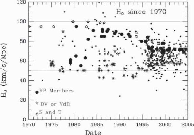
Figure 2: Various values of Hubble’s constant in units of kms sec^-1 Mpc^-1 plotted as a function of the date of publication. Labels refer to estimates by Sandage & Tammann, de Vaucouleurs, van den Bergh and their respective collaborators. Estimates from the HST Key Project group (Freedman et al 2001) are labeled KP. From an initial range spanning 50$<H_{0}<$100, a gradual convergence to the presently-accepted value is apparent. (Plot compiled and kindly made available by J. Huchra)

Figure 3 shows the two stage ‘step-ladder’ technique used by Freedman et al (2001) who claim a final value of 67 $\pm$ 15 kms sec^-1 Mpc^-1. ‘Primary’ distances were estimated to a set of nearby galaxies via the measured brightness and periods of luminous Cepheid variable stars located using HST’s WFPC-2 imager. Over the distance range across which such individual stars can be seen ($<$25 Mpc), the leverage on $H_{0}$ is limited and seriously affected by the peculiar motions of the individual galaxies. At $\simeq$20 Mpc, the smooth cosmic expansion would give $V_{exp}\simeq$1400 kms sec^-1 and a 10% error in $H_{0}$ would provide a comparable contribution, at this distance, to the typical peculiar motions of galaxies of $V_{pec}\simeq$50-100 kms sec^-1. Accordingly, a secondary distance scale was established for spirals to 400 Mpc distance using the empirical relationship first demonstrated by Tully & Fisher (1977) between the $I$-band luminosity and rotational velocity. At 400 Mpc, the effect of $V_{pec}$ is negligible and the leverage on $H_{0}$ is excellent. Independent distance estimators utilizing supernovae and elliptical galaxies were used to verify possible systematic errors.

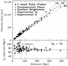
Figure 3: Two step approach to measuring Hubble’s constant $H_{0}$ - the local expansion rate (Freedman et al 2001). (Left) Distances to nearby galaxies within 25 Mpc were obtained by locating and monitoring Cepheid variables using HST’s WFPC-2 camera; the leverage on $H_{0}$ is modest over such small distances and affected seriously by peculiar motions. (Right) Extension of the distance-velocity relation to 400 Mpc using the I-band Tully-Fisher relation and other techniques. The absolute scale has been calibrated using the local Cepheid scale.

Cosmic Microwave Background: Thermal Origin and Spatial Flatness

The second significant milestone of the last 15 years is the improved understanding of the cosmic microwave background (CMB) radiation, commencing with the precise black body nature of its spectrum (Mather et al 1990) indicative of its thermal origin as a remnant of the cosmic fireball, and the subsequent detection of fluctuations (Smoot et al 1992), both realized with the COBE satellite data. The improved angular resolution of later ground-based and balloon-borne experiments led to the isolation of the acoustic horizon scale at the epoch of recombination (de Bernadis et al 2000, Hanany et al 2000). Subsequent improved measures of the angular power spectrum by the Wilkinson Microwave Anisotropy Probe (WMAP, Spergel et al 2003, 2006) have refined these early observations. The location of the primary peak in the angular power spectrum at a multiple moment $l\simeq$200 (corresponding to a physical angular scale of $\simeq$1 degree) provides an important constraint on the total energy density $\Omega_{TOT}$ and hence spatial curvature.

The derivation of spatial curvature from the angular location of the first acoustic (or ‘Doppler’) peak, $\theta_{H}$, is not completely independent of other cosmological parameters. There are dependences on the scale factor via $H_{0}$ and the contribution of gravitating matter $\Omega_{M}$, viz:

$$\theta_{H}\propto(\Omega_{M}\,h^{3.4})^{0.14}\,\Omega_{TOT}^{1.4}$$

where $h$ is $H_{0}$ in units of 100 kms sec^-1 Mpc^-1.

However, in the latest WMAP analysis, combining with distant supernovae data, space is flat to within 1%.

Clustering of Galaxies: Gravitational Instability

Galaxies represent the most direct tracer of the rich tapestry of structure in the local Universe. The 1970’s saw a concerted effort to introduce a formalism for describing and interpreting their statistical distribution through angular and spatial two point correlation functions (Peebles 1980). This, in turn, led to an observational revolution in cataloging their distribution, first in 2-D from panoramic photographic surveys aided by precise measuring machines, and later in 3-D from multi–object spectroscopic redshift surveys.

The angular correlation function $w(\theta)$ represents the excess probability $\delta\,P$ of finding a pair of galaxies separated by an angular separation $\theta$ (degrees).

In a catalog averaging $N$ galaxies per square degree, the probability of finding a pair separated by $\theta$ can be written:

$$\delta\,P=N[1+w(\theta)]\delta\,\Omega$$

where $\delta\,\Omega$ is the solid angle of the counting bin, (i.e. $\theta$ to $\theta+\delta\,\theta$).

The corresponding spatial equivalent, $\xi(r)$ in a catalog of mean density $\rho$ per Mpc³ is thus:

$$\delta\,P=\rho[1+\xi(r)]\delta\,V$$

One can be statistically linked to the other if the overall redshift distribution of the sources is available.

Figure 4 shows a pioneering detection of the angular correlation function $w(\theta)$ for the Cambridge APM Galaxy Catalog (Maddox et al 1990). This was one of the first well-constructed panoramic 2-D catalogs from which the large scale nature of the galaxy distribution could be discerned. A power law form is evident:

$$w(\theta)=A\theta^{-0.8}$$

where, for example, $\theta$ is measured in degrees. The amplitude $A$ decreases with increasing depth due to both increased projection from physically-uncorrelated pairs and the smaller projected physical scale for a given angle.

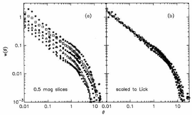
Figure 4: Angular correlation function for the APM galaxy catalog - a photographic survey of the southern sky (Maddox et al 1990) - partitioned according to limiting magnitude (left). The amplitude of the clustering decreases with increasing depth due to an increase in the number of uncorrelated pairs and a smaller projected physical scale for a given angle. These effects can be corrected in order to produce a high signal/noise function scaled to a fixed depth clearly illustrating a universal power law form over nearly 3 dex (right).

Highly-multiplexed spectrographs such as the 2 degree field instrument on the Anglo-Australian Telescope (Colless et al 2001) and the Sloan Digital Sky Survey (York et al 2001) have led to the equivalent progress in 3-D surveys (Figure 5). In the early precursors to these grand surveys, the 3-D equivalent of the angular correlation function, was also found to be a power law:

$$\xi(r)=(\frac{r}{r_{0}})^{-1.8}$$

where $r_{o}$ (Mpc) is a valuable clustering scale length for the population.

As the surveys became more substantial, the power spectrum $P(k)$ has become the preferred analysis tool because its form can be readily predicted for various dark matter models. For a given density field $\rho({\bf x})$, the fluctuation over the mean is $\delta=\rho\,/\,\overline{\rho}$ and for a given wavenumber $k$, the power spectrum becomes:

$$P(k)=<|\delta_{k}^{2}|>=\int\xi(r)exp(i{\bf k.r})d^{3}r$$

The final power spectrum for the completed 2dF survey is shown in Figure 6 (Cole et al 2005) and is in remarkably good agreement with that predicted for a cold dark matter spectrum consistent with that which reproduces the CMB angular fluctuations.

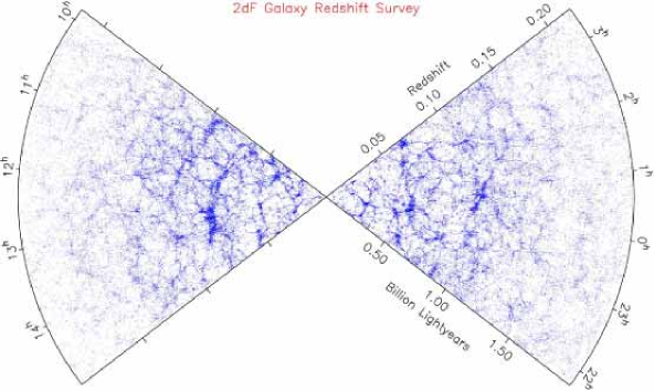
Figure 5: Galaxy distribution from the completed 2dF redshift survey (Colless et al 2001).

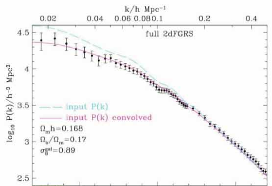
Figure 6: Power spectrum from the completed 2dF redshift survey (Cole et al 2005). Solid lines refer to the input power spectrum for a dark matter model with the tabulated parameters and that convolved with the geometric ‘window function’ which affects the observed shape on large scales.

Dark Matter and Gravitational Instability

We have already mentioned the ubiquity of dark matter on both cluster and galactic scales. The former was recognized as early as the 1930’s from the high line of sight velocity dispersion $\sigma_{los}$ of galaxies in the Coma cluster (Zwicky 1933). Assuming simple virial equilibrium and isotropically-arranged galaxy orbits, the cluster mass contained with some physical scale $R_{cl}$ is:

$$M=3<\sigma_{los}^{2}>R_{cl}/G$$

which far exceeds that estimated from the stellar populations in the cluster galaxies. High cluster masses can also be confirmed completely independently from gravitational lensing where a background source is distorted to produce a ‘giant arc’ - in effect a partial or incomplete ‘Einstein ring’ whose diameter $\theta_{E}$ for a concentrated mass $M$ approximates:

$$\theta_{E}=\frac{4GM^{\frac{1}{2}}}{c^{2}}\,D^{\frac{1}{2}}$$

and $D=D_{s}\,D_{l}\/,/\,D_{ds}$ where the subscripts $s$ and $l$ refer to angular diameters distances of the background source and lens respectively.

On galactic scales, extended rotation curves of gaseous emission lines in spirals (see review by Rubin 2000) can trace the mass distribution on the assumption of circular orbits, viz:

$$\frac{GM(<R)}{R^{2}}=\frac{V^{2}}{R}$$

Flat rotation curves ($V\sim$constant) thus imply $M(<R)\propto\,R$. Together with arguments based on the question on the stability of flattened disks (Ostriker & Peebles 1973), such observations were critical to the notion that all spiral galaxies are embedded in dark extensive ‘halos’.

The evidence for halos around local elliptical galaxies is less convincing largely because there are no suitable tracers of the gravitational potential on the necessary scales (see Gerhard et al 2001). However, by combining gravitational lensing with stellar dynamics for intermediate redshift ellipticals, Koopmans & Treu (2003) and Treu et al (2006) have mapped the projected dark matter distribution and show it to be closely fit by an isothermal profile $\rho(r)\propto r^{-2}$.

The presence of dark matter can also be deduced statistically from the distortion of the galaxy distribution viewed in redshift space, for example in the 2dF survey (Peacock et al 2001). The original idea was discussed by Kaiser et al (1987). The spatial correlation function $\xi(r)$ is split into its two orthogonal components, $\xi(\sigma,\pi)$ where $\sigma$ represents the projected separation perpendicular to the line of sight (unaffected by peculiar motions) and $\pi$ is the separation along the line of sight (inferred from the velocities and hence used to measure the effect). The distortion of $\xi(\sigma,\pi)$ in the $\pi$ direction can be measured on various scales and used to estimate the line of sight velocity dispersion of pairs of galaxies and hence their mutual gravitational field. Depending on the extent to which galaxies are biased tracers of the density field, such tests indicate $\Omega_{M}$=0.25.

On the largest scales, weak gravitational lensing can trace the overall distribution and dark matter content of the Universe (Blandford & Narayan 1992, Refregier 2003). Recent surveys are consistent with these estimates (Hoekstra et al 2005).

Dark Energy and Cosmic Acceleration

Prior to the 1980’s observational cosmologists were obsessed with two empirical quantities though to govern the cosmic expansion history – $R(t)$: Hubble’s constant $H_{0}=dR/dt$ and a second derivative, the deceleration parameter $q_{0}$, which would indicate the fate of the expansion:

$$q_{0}=-\frac{d^{2}R/dt^{2}}{(dR/dt)^{2}}$$

In the presence only of gravitating matter, Friedmann cosmologies indicate $\Omega_{M}=2\,q_{0}$. The distant supernovae searches were begun in the expectation of measuring $q_{0}$ independently of $\Omega_{M}$ and verifying a low density Universe.

As we have discussed, Type Ia supernovae (SNe) were found to be fainter at a given recessional velocity than expected in a Universe with a low mass density; Figure 7 illustrates the effect for the latest results from the Canada-France SN Legacy Survey (Astier et al 2006). In fact the results cannot be explained even in a Universe with no gravitating matter! A formal fit for $q_{0}$ indicates a negative value corresponding to a cosmic acceleration.

Acceleration is permitted in Friedmann models with a non-zero cosmological constant $\Lambda$. In general (Caroll et al 1992):

$$q_{0}=\frac{\Omega_{M}}{2}-3\,\frac{\Omega_{\Lambda}}{2}$$

where $\Omega_{\Lambda}=\Lambda/8\pi\,G$ is the energy density associated with the cosmological constant.

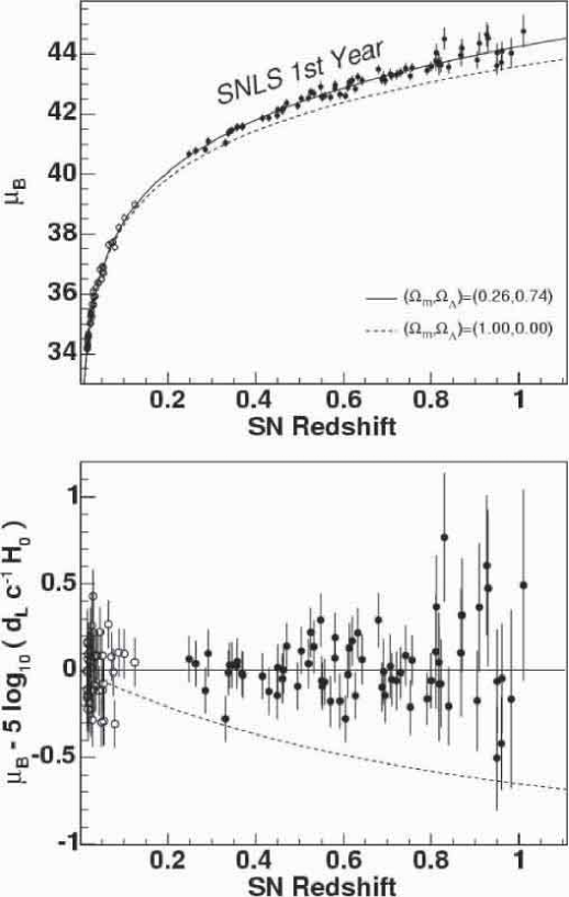
Figure 7: Hubble diagram (distance-redshift relation) for calibrated Type Ia supernovae from the first year data taken by the Canada France Supernova Legacy Survey (Astier et al 2006). Curves indicate the relation expected for a high density Universe without a cosmological constant and that for the concordance cosmology (see text)

The appeal of resurrecting the cosmological constant is not only its ability to explain the supernova data but also the spatial flatness in the acoustic peak in the CMB through the combined energy densities $\Omega_{M}+\Omega_{\Lambda}$ - the so-called Concordance Model (Ostriker & Steinhardt 1995, Bahcall et al 1999).

However, the observed acceleration raises many puzzles. The absolute value of the cosmological constant cannot be understood in terms of physical descriptions of the vacuum energy density, and the fact that $\Omega_{M}\simeq\Omega_{\Lambda}$ implies the accelerating phase began relatively recently (at a redshift of z$\simeq$0.7). Alternative physical descriptions of the phenomenon (termed ‘dark energy’) are thus being sought which can be generalized by imagining the vacuum obeys an equation of state where the negative pressure $p$ relates to the energy density $\rho$ via an index $w$,

$$p=w\,\rho$$

in which case the dependence on the scale factor $R$ goes as

$$\rho\propto R^{-3(1+w)}$$

The case $w$=-1 would thus correspond to a constant term equivalent to the cosmological constant, but in principle any $w<$-1/3 would produce an acceleration and conceivably $w$ is itself a function of time. The current SNLS data indicate $w$=-1.023 $\pm$ 0.09 and combining with the WMAP data does not significantly improve this constraint.

1.4 Concordance Cosmology: Why is such a curious model acceptable?

According to the latest WMAP results (Spergel et al 2006) and the analysis which draws upon the progress reviewed above (the HST Hubble constant Key Project, the large 2dF and SDSS redshift surveys, the CFHT supernova survey and the first weak gravitational lensing constraints), we live in a universe with the constituents listed in Table 1.

Table 1: Cosmic Constituents

Total Matter	$\Omega_{M}$	0.24 $\pm$ 0.03
Baryonic Matter	$\Omega_{B}$	0.042 $\pm$ 0.004
Dark Energy	$\Omega_{\Lambda}$	0.73 $\pm$ 0.04

Given only one of the 3 ingredient is physically understood it may be reasonably questioned why cosmologists are triumphant about having reached the era of ‘precision cosmology’! Surely we should not confuse measurement with understanding?

The underlying reasons are two-fold. Firstly, many independent probes (redshift surveys, CMB fluctuations and lensing) indicate the low matter density. Two independent probes not discussed (primordial nucleosynthesis and CMB fluctuations) support the baryon fraction. Finally, given spatial flatness, even if the supernovae data were discarded, we would deduce the non-zero dark energy from the above results alone.

Secondly, the above parameters reconcile the growth of structure from the CMB to the local redshift surveys in exquisite detail. Numerical simulations based on 10¹⁰ particles (e.g. Springel et al 2005) have reached the stage where they can predict the non-linear growth of the dark matter distribution at various epochs over a dynamic range of 3-4 dex in physical scales. Although some input physics is needed to predict the local galaxy distribution, the agreement for the concordance model (often termed $\Lambda$CDM) is impressive. In short, a low mass density and non-zero $\Lambda$ both seem necessary to explain the present abundance and mass distribution of galaxies. Any deviation would either lead to too much or too little structure.

This does not mean that the scorecard for $\Lambda$CDM should be considered perfect at this stage. As discussed, we have little idea what the dark matter or dark energy might be. Moreover, there are numerous difficulties in reconciling the distribution of dark matter with observations on galactic and cluster scales and frequent challenges that the mass assembly history of galaxies is inconsistent with the slow hierarchical growth expected in a $\Lambda$-dominated Universe. However, as we will see in later lectures, most of these problems relate to applications in environments where dark matter co-exists with baryons. Understanding how to incorporate baryons into the very detailed simulations now possible is an active area where interplay with observations is essential. It is helpful to view this interplay as a partnership between theory and observation rather than the oft-quoted ‘battle’ whereby observers challenge or call into question the basic principles.

1.5 Lecture Summary

I have spent my first lecture discussing largely cosmological progress and the impressive role that observations have played in delivering rapid progress.

All the useful cosmological functions - e.g. time, distance and comoving volume versus redshift, are now known to high accuracy which is tremendously beneficial for our task in understanding the first galaxies and stars. I emphasize this because even a decade ago, none of the physical constants were known well enough for us to be sure, for example, the cosmic age corresponding to a particular redshift.

I have justified $\Lambda\,CDM$ as an acceptable standard model, despite the unknown nature of its two dominant constituents, partly because there is a concordance in the parameters when viewed from various observational probes, and partly because of the impressive agreement with the distribution of galaxies on various scales in the present Universe.

Connecting the dark matter distribution to the observed properties of galaxies requires additional physics relating to how baryons cool and form stars in dark matter halos. Detailed observations are necessary to ‘tune’ the models so these additional components can be understood.

All of this will be crucial if we are correctly predict and interpret signals from the first objects.

2 Galaxies & the Hubble Sequence

2.1 Introduction: Changing Paradigms of Galaxy Formation

We now turn to the interesting history of how our views of galaxy formation have changed over the past 20-30 years. It is convenient to break this into 3 eras

1. The classical era (pre-1985) as articulated for example in the influential articles by Beatrice Tinsley and others. Galaxies were thought to evolve in isolation with their present-day properties governed largely by one function - the time-dependent star formation rate $\psi(t)$. Ellipticals suffered a prompt conversion of gas into stars, whereas spirals were permitted a more gradual consumption rate leading to a near-constant star formation rate with time.

2. The dark matter-based era (1985-): in hierarchical models of structure formation involving gravitational instability, the ubiquity of dark matter halos means that merger driven assembly is a key feature. If mergers redistribute angular momentum, galaxy morphologies are transformed.

3. Understanding feedback and the environment (1995-): In the most recent work, the evolution of the morphology-density relation (Dressler et al 1997) and the dependence of the assembly history on galactic mass (‘downsizing’, Cowie et al 1996) have emphasized that star formation is regulated by processes other than gas cooling and infall associated with DM-driven mergers.

2.2 Galaxy Morphology - Valuable Tool or Not?

In the early years, astronomers placed great stock on understanding the origin of the morphological distribution of galaxies, sometimes referred to as the Hubble sequence (Hubble 1936). Despite this simple categorization 70 years ago, the scheme is evidently still in common use. In its support, Sandage (e.g. 2005) has commented on this classification scheme as describing ‘a true order among the galaxies, not one imposed by the classifier’. However, many contemporary modelers and observers have paid scant attention to morphology and placed more emphasis on understanding stellar population differences. What value should we place on accurately measuring and reproducing the morphological distribution?

The utility of Hubble’s scheme, at least for local galaxies, lies in its ability to distinguish dynamically distinct structures - spirals and S0s are rotating stellar disks, whereas luminous spheroids are pressure-supported ellipsoidal or triaxial systems with anisotropic velocity fields. This contains key information on the degree of dissipation in their formation (Fall & Efstathiou 1980).

There are also physical variables that seem to underpin the sequence, including (i) gas content and color which relate to the ratio of the current to past average star formation ratio $\psi(t_{0})/\,\overline{\psi}$ (Figure 8) and (ii) inner structures including the bulge-to-disk ratio. Various modelers (Baugh et al 1996) have argued that the bulge-to-disk ratio is closely linked to the merger history and attempted to reproduce the present distribution as a key test of hierarchical assembly.

Figure 8: A succinct summary of the classical view of galaxy formation (pre-1985): (Left) The monotonic distribution of Hubble sequence galaxies in the $U-V$ vs $V-K$ color plane (Aaaronson 1978). (Right) A simple model which reproduces this trend by changing only the ratio of the current to past average star formation rate (Struck-Marcell & Tinsley 1978). Galaxies with constant star formation permanently occupy the top left (blue) corner; galaxies with an initial burst rapidly evolve to the bottom right (red) corner.

Much effort has been invested in attempting to classify galaxies at high redshift, both visually and with automated algorithms. This is a challenging task because the precise appearance of diagnostic features such as spiral arms and the bulge/disk ratio depends on the rest-wavelength of the observations. An effect termed the ‘morphological k-correction’ can thus shift galaxies to apparently later types as the redshift increases for observations conducted in a fixed band. A further limitation, which works in the opposite sense, is surface brightness dimming, which proceeds as $\propto\,(1+z)^{4}$, rendering disks less prominent at high redshift and shifting some galaxies to apparent earlier types.

The most significant achievements from this effort has been the realization that, despite the above quantitative uncertainties, faint star-forming galaxies are generally more irregular in their appearance than in local samples (Glazebrook et al 1995, Driver et al 1995). Moreover, HST images suggest on-going mergers with an increasing frequency at high redshift (LeFevre et al 2000) although quantitative estimates of the merging fraction as a function of redshift remain uncertain (see Bundy et al 2004).

The idea that morphology is driven by mergers took some time for the observational community to accept. Numerical simulations by Toomre & Toomre (1972) provided the initial theoretical inspiration, but the observational evidence supporting the notion that spheroidal galaxies were simple collapsed systems containing old stars was strong (Bower et al 1992). Tell-tale signs of mergers in local ellipticals include the discovery of orbital shells (Malin & Carter 1980) and multiple cores revealed only with 2-D dynamical studies (Davies et al 2001).

2.3 Semi-Analytical Modeling

As discussed by the other course lecturers and briefly in $\S$1, our ability to follow the distribution of dark matter and its growth in numerical simulations is well-advanced (e.g. Springel et al 2005). The same cannot be said of understanding how the baryons destined, in part, to become stars are allocated to each DM halo. This remains the key issue in interfacing theory to observations.

Progress has occurred in two stages - according to the eras discussed in §2.1. Semi analytic codes were first developed in the 1990’s to introduce baryons into DM n-body simulations using prescriptive methods for star formation, feedback and morphological assembly (Figure 9). These codes were initially motivated to demonstrate that the emerging DM paradigm was consistent with the abundance of observational data (Kauffmann et al 1993, Somerville & Primack 1999, Cole et al 2000). Prior to development of these codes, evolutionary predictions were based almost entirely on the ‘classical’ viewpoint with stellar population modeling based on variations in the star formation history $\psi(t)$ for galaxies evolving in isolation e.g. Bruzual (1980).

Figure 9: Schematic of the ingredients inserted into a semi-analytical model (from Cole et al 2000). Solid lines refer to mass transfer, dashed lines to the transfer of metals according to different compositions $Z$. Gas cooling ($\dot{M}$) and star formation ($\psi$) is inhibited by the effect of supernovae ($\beta$). Stars return some fraction of their mass to the interstellar medium ($R$) and to the hot gas phase ($e$) according to a metal yield $p$.

Initially these feedback prescriptions were adjusted to match observables such as the luminosity function (whose specific details we will address below), as well as specific attributes of various surveys (counts, redshift distributions, colors and morphologies). In the recent versions, more elaborate physically-based models for feedback processes are being considered (e.g. Croton et al 2006)

The observational community was fairly skeptical of the predictions from the first semi-analytical models since it was argued that the parameter space implied by Figure 9 enabled considerable freedom even for a fixed primordial fluctuation spectrum and cosmological model. Moreover, where different codes could be compared, considerably different predictions emerged (Benson et al 2002). Only as the observational data has moved from colors and star formation rates to physical variables more closely related to galaxy assembly (such as stellar masses) have the limitations of the early semi-analytical models been exposed.

2.4 A Test Case: The Galaxy Luminosity Function

One of the most straightforward and fundamental predictions a theory of galaxy formation can make is the present distribution of galaxy luminosities - the luminosity function (LF) $\Phi(L)$ whose units are normally per comoving Mpc³ .

As the contribution of a given luminosity bin $dL$ to the integrated luminosity density per unit volume is $\propto\Phi(L)\,L\,dL$, an elementary calculation shows that all luminosity functions (be they for stars, galaxies or QSOs) must have a bend at some characteristic luminosity, otherwise they would yield an infinite total luminosity (see Felton 1977 for a cogent early discussion of the significance and intricacies of the LF). Recognizing this, Schechter (1976) proposed the product of a power law and an exponential as an appropriate analytic representation of the LF, viz:

$$\Phi(L)\frac{dL}{L^{\ast}}=\Phi^{\ast}(\frac{L}{L^{\ast}})^{-\alpha}\,exp(-\frac{L}{L^{\ast}})\,\frac{dL}{L^{\ast}}$$

where $\Phi^{\ast}$ is the overall normalization corresponding to the volume density at the turn-over (or characteristic) luminosity $L^{\ast}$, and $\alpha$ is the faint end slope which governs the relative abundance of faint and luminous galaxies.

The total abundance of galaxies per unit volume is then:

$$N_{TOT}=\int\Phi(L)\,dL=\Phi^{\ast}\,\Gamma(\alpha+1)$$

and the total luminosity density is:

$$\rho_{L}=\int\Phi(L)\,L\,dL=\Phi^{\ast}\,\Gamma(\alpha+2)$$

where $\Gamma$ is the incomplete gamma function which can be found tabulated in most books with integral tables (e.g. Gradshteyn & Ryzhik 2000). Note that $N_{TOT}$ diverges if $\alpha<$-1, whereas $\rho_{L}$ diverges only if $\alpha<$-2.

Recent comprehensive surveys by the 2dF team (Norberg et al 2002) and by the Sloan Digital Sky Survey (Blanton et al 2001) have provided definitive values for the LF in various bands. Encouragingly, when allowance is made for the various photometric techniques, the two surveys are in excellent agreement. Figure 10 shows the Schechter function is a reasonably good (but not perfect) fit to the 2dF data limited at apparent magnitude $b_{J}<$19.7. Moreover there is no significant difference between the LF derived independently for the two Galactic hemispheres. The slight excess of intrinsically faint galaxies in the northern cap is attributable to a local inhomogeneity in the nearby Virgo supercluster.

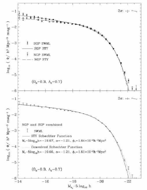
Figure 10: Rest-frame $b_{J}$ luminosity function from the 2dF galaxy redshift survey (Norberg et al 2002). (Top) a comparison of results across the northern and southern Galactic caps; there is only a marginal difference in the abundance of intrinsically faint galaxies. (Bottom) combined from both hemispheres indicating the Schechter function is a remarkably good fit except at the extreme ends of the luminosity distribution.

Fundamental though this function is, despite ten years of semi-analytical modeling, reproducing its form has proved a formidable challenge (as discussed by Benson et al 2003, Croton et al 2006 and de Lucia et al 2006). Early predictions also failed to reproduce the color distribution along the LF. The halo mass distribution does not share the sharp bend at $\L^{\ast}$ and too much star formation activity is retained in massive galaxies. These early predictions produced too many luminous blue galaxies and too many faint red galaxies (Bower et al 2006).

As a result, more specific feedback recipes have been created to resolve this discrepancy. Several physical processes have been invoked to regulate star formation as a function of mass, viz:

• Reionization feedback: radiative heating from the first stellar systems at high redshift which increases the Jeans mass, inhibiting the early formation of low mass systems,

• Supernova feedback: this was considered in the early semi-analytical models but is now more precisely implemented so as to re-heat the interstellar medium, heat the halo gas or even eject the gas altogether from low mass systems,

• Feedback from active galactic nuclei: the least well-understood process with various modes postulated to transfer energy from an active nucleus to the halo gas.

Benson et al (2003) and Croton et al (2006) illustrate the effects of these more detailed prescriptions for these feedback modes on the predicted LF and find that supernova and reionization feedback largely reduce the excess of intrinsically faint galaxies but, on grounds of energetics, only AGN can inhibit star formation and continued growth in massive galaxies. There remains an excess at the very faint end (Fig. 11).

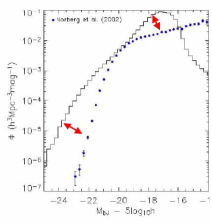
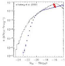
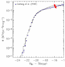
Figure 11: The effect of various forms of feedback (dots) on the resultant shape of the blue 2dF galaxy luminosity function (Norberg et al 2002). From left to right: no feedback, supernova feedback only, supernova, reionization & AGN feedback (Courtesy: Darren Croton).

2.5 The Role of the Environment

In addition to recognizing that more elaborate modes of feedback need to be incorporated in theoretical models, the key role of the environment has also emerged as an additional feature which can truncate star formation and alter galaxy morphologies.

The preponderance of elliptical and S0 galaxies in rich clusters was noticed in the 1930’s but the first quantitative study of this effect was that of Dressler (1980) who correlated the fraction of galaxies of a given morphology $T$ above some fixed luminosity with the projected galaxy density, $\Sigma$, measured in galaxies Mpc^-2.

The local $T-\Sigma$ relation was used to justify two rather different possibilities. In the first, the nature hypothesis, those galaxies which formed in high density peaks at early times were presumed to have consumed their gas efficiently, perhaps in a single burst of star formation. Galaxies in lower density environments continued to accrete gas and thus show later star formation and disk-like morphologies. In short, segregation was established at birth and the present relation simply represents different ways in which galaxies formed according to the density of the environment at the time of formation. In the second, the nurture hypothesis, galaxies are transformed at later times from spirals into spheroidals by environmentally-induced processes.

Work in the late 1990’s, using morphologies determined using Hubble Space Telescope, confirmed a surprisingly rapid evolution in the $T-\Sigma$ relation over 0$<z<$0.5 (Couch et al 1998, Dressler et al 1997) strongly supporting environmentally-driven evolution along the lines of the nurture hypothesis. Impressive Hubble images of dense clusters at quite modest redshifts ($z\simeq$0.3-0.4) showed an abundance of spirals in their cores whereas few or none exist in similar environs today.

What physical processes drive this relation and how has the $T-\Sigma$ relation evolved in quantitative detail? Recent work (Smith et al 2005, Postman et al 2005, Figure 12) has revealed that the basic relation was in place at $z\simeq$1, but that the fraction $f_{E+S0}$ of Es and S0s has doubled in dense environments since that time. Smith et al suggest that a continuous, density-dependent, transformation of spirals into S0s would explain the overall trend. Treu et al (2003) likewise see a strong dependence of the fraction as a function of $\Sigma$ (and to a lesser extent with cluster-centric radius) within a well-studied cluster at $z\simeq$0.4; they review the various physical mechanisms that may produce such a transformation.

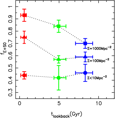
Figure 12: The fraction of observed E and S0 galaxies down to a fixed rest-frame luminosity as a function of lookback time and projected density $\Sigma$ from the study of Smith et al (2005). Although the morphology density relation was already in place at $z\simeq$1, there has been a continuous growth in the fraction subsequently, possibly as a result of the density-dependent transformation of spirals into S0s.

Figure 12 encapsulates much of what we now know about the role of the environment on galaxy formation. The early development of the $T-\Sigma$ relation implies dense peaks in the dark matter distribution led to accelerated evolution in gas consumption and stellar evolution and this is not dissimilar to the nature hypothesis. However, the subsequent development of this relation since $z\simeq$1 reveals the importance of environmentally-driven morphological transformations.

2.6 The Importance of High Redshift Data

This glimpse of evolving galaxy populations to $z\simeq$1 has emphasized the important role of high redshift data. In the case of the local morphology-density relation, Hubble morphologies of galaxies in distant clusters have given us a clear view of an evolving relationship, partly driven by environmental processes. Indeed, the data seems to confirm the nurture hypothesis for the origin of the morphology-density relation.

Although we can place important constraints on the past star formation history from detailed studies of nearby galaxies, as the standard model now needs several additional ingredients (e.g. feedback) to reproduce even the most basic local properties such as the luminosity function (Figure 11), data at significant look-back times becomes an essential way to test the validity of these more elaborate models.

Starting in the mid-1990’s, largely by virtue of the arrival of the Keck telescopes - the first of the new generation of 8-10m class optical/infrared telescopes - and the refurbishment of the Hubble Space Telescope, there has been an explosion of new data on high redshift galaxies.

It is helpful at this stage to introduce three broad classes of distant objects which will feature significantly in the next few lectures. Each gives a complementary view of the galaxy population at high redshift and illustrates the challenge of developing a unified vision of galaxy evolution.

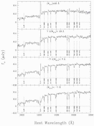
Figure 13: Location and verification of the Lyman break population in the redshift range 2.7$<z<$3.4 (Steidel et al 2003). (Left) $UGR$ color-color plane for a single field; green and yellow shading refers to variants on the color selection of high redshift candidates. Contaminating Galactic stars cut across the lower right corner of this selection; those confirmed spectroscopically are marked in red. (Right) Coadded rest-frame Keck spectra for samples of typically 200 Lyman break galaxies binned according to the strength of Lyman $\alpha$ emission.

• Lyman-break galaxies: color-selected luminous star forming galaxies at $z>$2. First located spectroscopically by Steidel et al (1996, 1999a, 1999b, 2003), these sources are selected by virtue of the increased opacity shortward of the Lyman limit ($\lambda=$912Å ) arising from the combined effect of neutral hydrogen in hot stellar atmospheres, the interstellar gas and the intergalactic medium. When redshifted beyond z$\simeq$2, the characteristic ‘drop out’ in the Lyman continuum moves into the optical (Figure 13). We will review the detailed properties of this, the most well-studied, distant galaxy population over 2$<z<$5 in subsequent lectures.

  

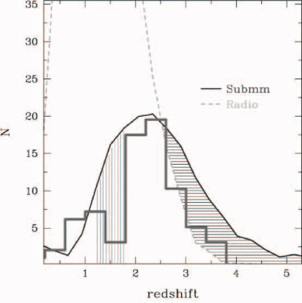
  Figure 14: Redshift distribution of 73 radio-identified SCUBA sources from Chapman et al (2005). To illustrate the possible bias arising from the necessary condition of a radio position for a Keck redshift, the solid curve represents a model prediction for the entire $>$5mJy sub-mm population. The sub-mm population does not seem to extend significantly beyond z$\simeq$4 and has a median redshift of $z$=2.2.

• Sub-millimeter star forming sources: The SCUBA 850$\mu$m array on the 15 meter James Clerk Maxwell Telescope and other sub-mm imaging devices have also been used to locate distant star forming galaxies (Smail et al 1997, Hughes et al 1998). In this case, emission is detected from dust, heated either by vigorous star formation or an active nucleus. Remarkably, their visibility does not fall off significantly with redshift because they are detected in the Rayleigh-Jeans tail of the dust blackbody spectrum (Blain et al 2002).

  Progress in understanding the role and nature of this population has been slower because sub-mm sources are often not visible at optical and near-infrared wavelengths (due to obscuration) and the positional accuracy of the sub-mm arrays is too coarse for follow-up spectroscopy. The importance of sub-mm sources lies in the fact that they contribute significantly to the star formation rate at high redshift. Regardless of their redshift, the source density at faint limits is 1000 times higher than a no-evolution prediction based on the local abundance of dusty IRAS sources. For several years the key issue was to nail the redshift distribution.

  Progress has been made by securing accurate positions using radio interferometers such as the VLA (Frayer et al 2000). About 70% of those brighter than 5 mJy have VLA detections and spectroscopic redshift have now been determined for a significant fraction of this population (Chapman et al 2003, 2005, Figure 14).

  

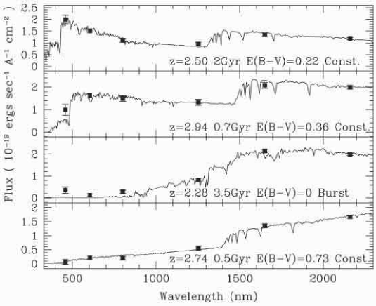
  Figure 15: Observed spectral energy distribution of distant red sources selected with a red $J-K$ color superimposed on model spectra (Franx et al 2003). Although some sources reveal modest star formation and can be spectroscopically confirmed to lie above $z\simeq$2, others (such as the lower two examples) appear to be passively-evolving with no active star formation.

• Passively-Evolving Sources: The Lyman-break and sub-mm sources are largely star-forming galaxies. The arrival of panoramic near-infrared cameras has opened the possibility of locating quiescent sources that are no longer forming stars. Such sources would not normally be detected via the other techniques and so understanding their contribution to the integrated stellar mass at, say, $z\simeq$2, is very important.

  The nomenclature here is confusing with intrinsically red sources being termed ‘extremely red objects (EROs)’ or ‘distant red galaxies (DRGs)’ with no agreed selection criteria (see McCarthy 2004 for a review). When star formation is complete, stellar evolution continues in a passive sense with main sequence dimming; the galaxy fades and becomes redder.

  Of particular interest are the most distant examples which co-exist alongside the sub-mm and Lyman-break galaxies, i.e. at $z>$2 selected according to their infrared $J-K$ color (van Dokkum et al 2003, Figure 15).

2.7 Lecture Summary

We have seen in this brief tour that galaxy formation is a process involving gravitational instability driven by the hierarchical assembly of dark matter halos; this component we understand well. However, additional complexities arise from star formation, dynamical interactions and mergers, environmental processes and various forms of feedback which serve to regulate how star formation continues as galaxies grow in mass.

Theorists have attempted to deal with this complexity by augmenting the highly-successful numerical (DM-only) simulations with semi-analytic tools for incorporating these complexities. As the datasets have improved so it is now possible to consider ‘fine-tuning’ these semi-analytical ingredients. Ab initio modeling is never likely to be practical.

I think it fair to say that many observers have philosophical reservations about this ‘fine-tuning’ process in the sense that although it may be possible to reach closure on models and data, we seek a deeper understanding of the physical reality of many of the ingredients. This is particularly the case for feedback processes. Fortunately, high redshift data forces this reality check as it gives us a direct measure of the galaxy assembly history which will be the next topics we discuss.

As a way of illustrating the importance of high redshift data, I have introduced three very different populations of galaxies each largely lying in the redshift range 2$<z<$4. When these were independently discovered, it was (quite reasonably) claimed by their discoverers that their category represented a major, if not the most significant, component of the distant galaxy population. We now realize that UV-selected, sub-mm selected and non-star forming galaxies each provide a complementary view of the complex history of galaxy assembly and the challenge is to complete the ‘jig-saw’ from these populations.

3 Cosmic Star Formation Histories

3.1 When Did Galaxies Form? Searches for Primeval Galaxies

The question of the appearance of an early forming galaxy goes back to the 1960’s. Partride & Peebles (1967) imagined the free-fall collapse of a 700 $\L^{\ast}$ system at $z\simeq$10 and predicted a diffuse large object with possible Lyman $\alpha$ emission. Meier (1976) considered primeval galaxies might be compact and intense emitters such as quasars.

In the late 1970’s and 1980’s when the (then) new generation of 4 meter telescopes arrived, astronomers sought to discover the distinct era when galaxies formed. Stellar synthesis models (Tinsley 1980, Bruzual 1980) suggested present-day passive systems (E/S0s) could have formed via a high redshift luminous initial burst. Placed at $z\simeq$2-3, sources of the same stellar mass would be readily detectable at quite modest magnitudes, $B\simeq$22-23, and provide an excess population of blue galaxies.

In reality, the (now well-studied) excess of faint blue galaxies over locally-based predictions is understood to be primarily a phenomenon associated with a gradual increase in star formation over $0<z<$1 rather than one due to a distinct new population of intensely luminous sources at high redshift (Koo & Kron 1992, Ellis 1997). Moreover, dedicated searches for suitably intense Lyman $\alpha$ emitters were largely unsuccessful. Pritchet (1994) comprehensively reviews a decade of searching.

Our thinking about primeval galaxies changed in two respects in the late 1980’s. Foremost, synthesis models such as those developed by Tinsley and Bruzual assumed isolated systems; dark matter-based models emphasized the gradual assembly of massive galaxies. This change meant that, at $z\simeq$2-3, the abundance of massive galaxies should be much reduced. Secondly, the flux limits searched for primeval galaxies were optimistically bright; we slowly realized the more formidable challenge of finding these enigmatic sources.

3.2 Local Inventory of Stars

An important constraint on the past star formation history is the present-day stellar density. The former must, when integrated, yield the latter. Fukugita et al (1998) and Fukugita & Peebles (2004) have considered this important problem based on local survey data provided by the SDSS (Kauffmann et al 2003) and 2dF (Cole et al 2001) redshift samples.

The derivation of the integrated density of stars involves many assumptions and steps but is based primarily on the local infrared ($K$-band) luminosity function of galaxies. The rest-frame $K$ luminosity of a galaxy is a much more reliable proxy for its stellar mass than that at a shorter (e.g. optical) wavelength because its value is largely irrespective of the past star formation history - a point illustrated by Kauffmann & Charlot (1998, Figure 16). Another way to phrase this is to say that the infrared mass/light ratio ($M/L_{K}$) is fairly independent of the star formation history, so that the stellar mass can be derived from the observed $K$-band luminosity by a multiplicative factor.

Figure 16: The robustness of the $K$-band luminosity of a galaxy as a proxy for stellar mass (Kauffmann & Charlot 1998). The upper panel shows the $K$-band apparent magnitude of a galaxy defined to have a fixed stellar mass of $10^{11}M_{\odot}$ when placed at various redshifts. The different curves represent extreme variations in the way the stellar population was created. Whereas the $B-K$ color is strongly dependent upon the star formation history, the $K$-band luminosity is largely independent of it.

In practice the mass/light ratio depends on the assumed distribution of stellar masses in a stellar population. The zero age or initial mass function is usually assumed to be some form of power law which can only be determined reliable for Galactic stellar populations, although constraints are possible for extragalactic populations from colors and nebular line emission (see reviews by Scalo 1986, Kennicutt 1998, Chabrier 2003)

In its most frequently-used form the IMF is quoted in mass fraction per logarithmic mass bin: viz:

$$\xi(log\,m)=\frac{dn}{d\,log\,m}\propto m^{-x}$$

or, occasionally,

$$\xi(m)=\frac{dn}{dm}=\frac{1}{m(ln\,10)}\xi(logm)\propto m^{-\alpha}$$

where $x=\alpha-1$.

In his classic derivation of the IMF, Salpeter (1955) determined a pure power law with $x$=1.35. More recently adopted IMFs are compared in Figure 17. They differ primarily in how to restrict the low mass contribution, but there is also some dispute on the high mass slope (although the Salpeter value is supported by various observations of galaxy colors and H$\alpha$ distributions, Kennicutt 1998).

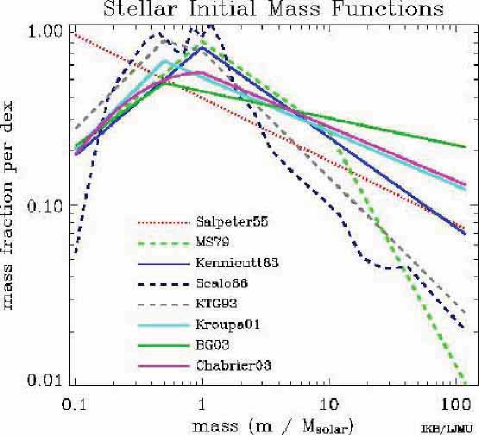
Figure 17: A comparison of popular stellar initial mass functions (courtesy of Ivan Baldry).

Table 2: K-band Stellar Mass/Light Ratios

Source	Stars	Stars + WDs/BHs	Total (Past SFR)
Salpeter (1955)	1.15	1.30	1.86
Miller Scalo (1979)	0.46	0.60	0.99
Kennicutt (1983)	0.46	0.60	1.06
Scalo (1986)	0.52	0.61	0.84
Kroupa et al (1993)	0.65	0.76	1.09
Kroupa (2001)	0.67	0.83	1.48
Baldry & Glazebrook (2003)	0.67	0.86	1.76
Chabrier (2003)	0.59	0.75	1.42

The IMF has a direct influence on the assumed $M/L_{K}$ (as discussed by Baldry & Glazebrook 2003, Chabrier, 2003 and Fukugita & Peebles, 2004) in a manner which depends on the age, composition and past star formation history. The adopted mass/light ratio is then a crucial ingredient for computing both stellar masses (LectureLecture 4) and galaxy colors.

Baldry has undertaken a very useful comparative study of the impact of various IMF assumptions using the PEGASE 2.0 stellar synthesis code for a population 10 Gyr old with solar metallicity, integrating between stellar masses of 0.1 and 120 $M_{\odot}$ (Table 2). Stellar masses have been defined in various ways as represented by the 3 columns in Table 2. Typically we are interested in the observable stellar mass at a given time (i.e. main sequence and giant branch stars), but it is interesting to also compute the total mass which is not in the interstellar medium, which includes that locked in evolved degenerate objects (white dwarfs and black holes). The most inclusive definition of stellar mass (total) is the integral of the past star formation history. Depending on the definition, and chosen IMF, the uncertainties range almost over a factor of 4 for the most popularly-used functions, quite apart from the unsettling question of whether the form of the IMF might vary with epoch or type of object.

Although the stellar mass function for a galaxy survey can be derived assuming a fixed mass/light ratio, the useful stellar density is that corrected for the fractional loss, $R$, of stellar material due to winds and supernovae. Only with this correction ($R$=0.28 for a Salpeter IMF), does the present-day value represent the integral of the past star formation.

Figure 18 shows the $K$-band luminosity and derived stellar mass function for galaxies in the 2dF redshift survey from the analysis of Cole et al (2001). $K$-band measures were obtained by correlation with the $K<$13.0 catalog obtained by the 2MASS survey.

Figure 18: (Left) Rest-frame $K$-band luminosity function derived from the combination of redshifts from the 2dF survey with photometry from 2MASS (Cole et al 2001); Schechter parameter fits are shown. (Right) Derived stellar mass function assuming a Salpeter IMF corrected for lost material assuming $R$=0.28 (see text).

The integrated stellar density, corrected for stellar mass loss, is (Cole et al 2001):

$$\Omega_{stars}\,h=0.0027\pm 0.00027$$

for a Salpeter IMF, a value very similar to that derived independently by Fukugita & Peebles (2004). By comparison the local mass fraction in neutral HI + He I gas is:

$$\Omega_{gas}\,h=0.00078\pm 0.00016$$

Thus only 5% of all baryons are in stars with the bulk in ionized gas.

3.3 Diagnostics of Star Formation in Galaxies

When significant redshift surveys became possible at intermediate and high redshift through the advent of multi-object spectrographs, so it became possible to consider various probes of the star formation rate (SFR) at different epochs. As in the formalism for calculating the integrated luminosity density, $\rho_{L}$, per comoving Mpc³, so for a given population various diagnostics of on-going star formation can yield an equivalent global star formation rate $\rho_{SFR}$ in units of $M_{\odot}$ yr^-1 Mpc^-3.

Such integrated measures average over a whole host of important details, such as differences in evolutionary behavior between luminous and sub-luminous galaxies and, of course, morphology. Moreover, in any survey at high redshift, only a portion of the population is rendered visible so uncertain corrections must be made to compare results at different epochs. The importance of the cosmic star formation history, i.e. $\rho_{SFR}(z)$, is it displays, in a simple manner, the epoch and duration of galaxy growth. By integrating the function, one should recover the present stellar density (§3.5).

There are various probes of star formation in galaxies, each with its advantages and drawbacks. Not only is there no single ‘best’ method to gauge the current star formation rate of a chosen galaxy, but as each probe samples the effect of young stars in different initial mass ranges, so each averages the star formation rate over a different time interval. If, as is often the case in the most energetic sources, the star formation is erratic or burst-like, one would not expect different diagnostics to give the same measure of the instantaneous SFR even for the same galaxies.

Four diagnostics are in common use (see review by Kennicutt 1998).

• The rest-frame ultraviolet continuum ($\lambda\lambda\simeq$1250-1500Å ) has the advantage of being directly connected to well-understood high mass ($>5M_{\odot}$) main sequence stars. Large datasets are available for high redshift star-forming galaxies, including some to $z\simeq$6. Via the GALEX satellite and earlier balloon-borne experiments, local data is also available. The disadvantage of this diagnostic lies in the uncertain (and significant) corrections necessary for dust extinction and a modest sensitivity to the assumed initial mass function. Obscured populations are completely missed in UV samples. Kennicutt suggests the following calibration for the UV luminosity:

  $$SFR(M_{\odot}yr^{-1})=1.4\,10^{-28}L_{\nu}(ergs\,s^{-1}Hz^{-1})$$

• Nebular emission lines such as $H\alpha$ and [O II] are also available for a range of redshifts ($z<2.5$), for example as a natural by-product of faint redshift surveys. Gas clouds are photo-ionized by very massive ($>10M_{\odot}$) stars. Dust extinction can often be evaluated from higher order Balmer lines under various radiative assumptions depending on the escape fraction of ionizing photons. The sensitivity to the initial mass function is strong.

  $$SFR(M_{\odot}yr^{-1})=7.9\,10^{-42}L(H\alpha)(ergs\,s^{-1})$$

  $$SFR(M_{\odot}yr^{-1})=1.4\pm 0.410^{-41}L(OII)(ergs\,s^{-1})$$

• Far infrared emission (10-300 $\mu$m) arises from dust heated by young stars. It is clearly only a tracer in the most dusty systems and thus acts as a valuable complementary probe to the UV continuum. As we have seen in §2, luminous far infrared galaxies are also seen to high redshift. However, not all dust heating is due to young stars and the bolometric far infrared flux, $L_{FIR}$, is needed for an accurate measurement.

  $$SFR(M_{\odot}yr^{-1})=4.5\,10^{-44}L_{FIR}(ergs\,s^{-1})$$

• Radio emission, e.g. at 1.4GHz, is thought to arise from synchrotron emission generated by relativistic electrons accelerated by supernova remnants following the rapid evolution of the most massive stars. Its great advantage is that it offers a dust-free measure of the recent SFR. Current radio surveys do not have the sensitivity to see emission beyond $z\simeq$1, so its promise has yet to be fully explored. This process is also the least well-understood and calibrated. Sullivan et al (2001) discuss this point in some detail and conclude:

  $$SFR(M_{\odot}yr^{-1})=1.1\,10^{-28}L_{1.4}(ergs\,s^{-1}Hz^{-1})$$

  for bursts of duration $>$100 Myr.

The question of the time-dependent nature of the SFR is an important point (Sullivan et al 2000, 2001). For an instantaneous burst of star formation, Figure 19a shows the ‘response’ of the various diagnostics. Clearly if the SF is erratic on 0.01-0.1 Gyr timescales, each will provide a different sensitivity. Sullivan et al (2000) compared UV and H$\alpha$ diagnostics for a large sample of nearby galaxies and found a scatter beyond that expected from the effects of dust extinction or observational error, presumably from this effect (Figure 19b).

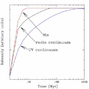
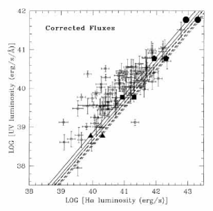
Figure 19: Time dependence of various diagnostics of star formation in galaxies. (Left) sensitivities for a single burst of star formation. (Right) scatter in the UV and H$\alpha$ galaxy luminosities in the local survey of Sullivan et al (2000); lines represent model predictions for various (constant) star formation rates and metallicities. It is claimed that some fraction of local galaxies must undergo erratic periods of star formation in order to account for the offset and scatter.

In addition to the initial mass function (already discussed), a key uncertainty affecting the UV diagnostic is the selective dust extinction law. Over the wavelength range 0.3$<\lambda<$1 $\mu$m, differences between laws deduced for the Milky Way, the Magellan clouds and local starburst galaxies (Calzetti et al 2000) are quite modest. Significant differences occur around the 2200 Å feature (dominant in the Milky Way but absence in Calzetti’s formula) and shortward of 2000 Å where the various formulae differ by $\pm$2 mags in $A(\lambda)/E(B-V)$.

3.4 Cosmic Star Formation - Observations

Early compilations of the cosmic star formation history followed the field redshift surveys of Lilly et al (1996), Ellis et al (1996) and the abundance of U-band drop outs in the early deep HST data (Madau et al 1996). The pioneering papers in this regard include Lilly et al (1996), Fall et al (1996) and Madau et al (1996, 1998).

Hopkins (2004) and Hopkins & Beacom (2006) have undertaken a valuable recent compilation, standardizing all measures to the same initial mass function, cosmology and extinction law. They have also integrated the various luminosity functions for each diagnostic in a self-consistent manner (except at very high redshift). Accordingly, their articles give us a valuable summary of the state of the art.

Figure 20 summarizes their findings. Although at first sight somewhat confusing, some clear trends are evident including a systematic increase in star formation rate per unit volume out to $z\simeq$1 which is close to (Hopkins 2004):

$$\rho_{SFR}(z)\propto(1+z)^{3.1}$$

A more elaborate formulate is fitted in Hopkins & Beacom (2006).

There is a broad peak somewhere in the region 2$<z<$4 where the UV data is consistently an underestimate and the growing samples of sub-mm galaxies are valuable. The dispersion here is only a factor of $\pm$2 or so, which is a considerable improvement on earlier work. We will return to the question of a possible decline in the cosmic SFR beyond $z\simeq$3-4 in later sections.

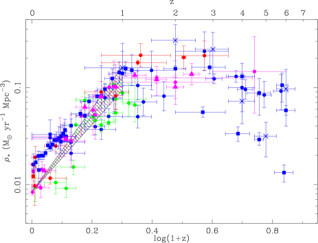
Figure 20: Recent compilations of the cosmic star formation history. Circles are data from Hopkins (2004) color-coded by method: blue: UV, green: [O II], red: H$\alpha/\beta$, magenta: non-optical including sub-mm and radio. New data from Hopkins & Beacom (2006), represented by various triangles, stars and squares, include Spitzer FIR measures (magenta triangles). The solid lines represent a range of the best fitting parametric form for $z<$1.

In their recent update, Hopkins & Beacom (2006) also parametrically fit the resulting $\rho_{SFR}(z)$ in two further redshift sections, beyond $z\simeq$1, and they use this to predict the growth of the absolute stellar mass density, $\rho_{\ast}$, via integration (Figure 21). Concentrating, for now, on the reproduction of the present day mass density (Cole et al 2001), the agreement is remarkably good.

Although in detail the result depends on an assumed initial mass function and the vexing question of whether extinction might be luminosity-dependent, this is an important result in two respects: firstly, as an absolute comparison it confirms that most of the star formation necessary to explain the presently-observed stellar mass has already been detected through various complementary surveys. Secondly, the study allows us to predict fairly precisely the epoch by which time half the present stellar mass was in place; this is $z_{\frac{1}{2}}=2.0\pm 0.2$. In §4 we will discuss this conclusion further attempting to verify it by measuring stellar masses of distant galaxies directly.

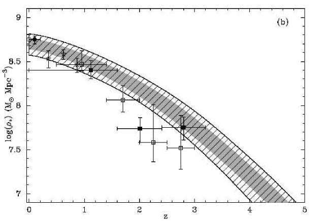
Figure 21: Growth of stellar mass density, $\rho_{\ast}$, with redshift obtained by direct integration of a parametric fit to the cosmic star formation history deduced by Hopkins & Beacom (2006, see Figure 20). The integration accurately reproduces the local stellar mass density observed by Cole et al (2001) and suggests half the present density was in place at $z$=2.0 $\pm$ 0.2.

3.5 Cosmic Star Formation - Theory

As we have discussed, semi-analytical models have had a hard time reproducing and predicting the cosmic star formation history. Amusingly, as the data has improved, the models have largely done a ‘catch-up’ job (Baugh et al 1998, 2005a). To their credit, while many observers were still convinced galaxies formed the bulk of their stars in a narrow time interval (the ‘primeval galaxy’ hypothesis), CDM theorists were the first to suggest the extended star formation histories now seen in Figure 20.

A particular challenge seems to be that of reproducing the abundance of energetic sub-mm sources whose star formation rates exceed 100-200 $M_{\odot}$ yr^-1. Baugh et al (2005b) have suggested it may require a combination of quiescent and burst modes of star formation, the former involving an initial mass function steepened towards high mass stars. Although there is much freedom in the semi-analytical models, recent models suggest $z_{\frac{1}{2}}\simeq 1.3$. By contrast, for the same cosmological models, hydrodynamical simulations (Nagamine et al 2004) predict much earlier star formation, consistent with $z_{\frac{1}{2}}\simeq 2.0-2.5$.

The flexibility of these models is considerable so my personal view is that not much can be learned from these comparisons either way. It is more instructive to compare galaxy masses at various epochs with theoretical predictions. Although we are still some ways from doing this in a manner that includes both baryonic and dark components, progress is already promising and will be reviewed in §4.

3.6 Unifying the Various High Redshift Populations

Integrating the various star-forming populations at high redshift to produce Figure 20 avoids the important question of the physical relevance and roles of the seemingly-diverse categories of high redshift galaxies. In the previous lecture (§2), I introduced three broad categories: the Lyman break (LBG), sub-mm and passively-evolving sources (DRGs) which co-exist over 1$<z<$3. What is the relationship between these objects?

As the datasets on each has improved, we have secured important physical variables including masses, star formation rates and ages. We can thus begin to understand not only their relative contributions to the SFR at a given epoch, but the degree of overlap among the various populations. Several recent articles have begun to evaluate the connection between these various categories (Papovich et al 2006, Reddy et al 2005).

A particularly valuable measure is the clustering scale, $r_{0}$, for each population, as defined in §1.3. This is closely linked to the halo mass according to CDM and thus sets a marker for connecting populations observed at different epochs. Adelberger et al (1998) demonstrated the strong clustering, $r_{0}\simeq$3.8 Mpc, of luminous LBGs at $z\simeq$3. Baugh et al (1998) claimed this was consistent with the progenitor halos of present-day massive ellipticals. The key to the physical nature of LBGs depends the origin of their intense star formation. At $z\simeq$3, the bright end of the UV luminosity function is $\simeq$1.5 mags brighter than its local equivalent; the mean SFR is 45 $M_{\odot}$ yr^-1. Is this due to prolonged activity, consistent with the build up of the bulk of stars which reside in present-day massive ellipticals, or is it a temporary phase due to merger-induced starbursts (Somerville et al 2001).

Shapley et al (2001, 2003) investigated the stellar population and stacked spectra of a large sample of $z\simeq$3 LBGs and find younger systems with intense SFRs are dustier with weaker Ly$\alpha$ emission while outflows (or ‘superwinds’) are present in virtually all (Figure 22a). For the young LBGs, a brief period of elevated star formation seems to coincide with a large dust opacity hinting at a possible overlap with the sub-mm sources. During this rapid phase, gas and dust is depleted by outflows leading to eventually to a longer, more quiescent phase during which time the bulk of the stellar mass is assembled.

If young dusty LBGs with SFRs $\simeq 300M_{\odot}$ yr^-1 represent a transient phase, we might expect sub-mm sources to simply be a yet rarer, more extreme version of the same phenomenon. The key to testing this connection lies in the relative clustering scales of the two populations (Figure 22b). Blain et al (2004) find sub-mm galaxies are indeed more strongly clustered than the average LBGs, albeit with some uncertainty given the much smaller sample size.

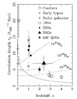
Figure 22: Connecting Lyman break and sub-mm sources. (Left) Correlation between the mean age (for a constant SFR) and reddening for a sample of $z\simeq$3 LBGs from the analysis of Shapley et al (2001). The youngest LGBs seem to occupy a brief dusty phase limited eventually by the effect of powerful galaxy-scale outflows. (Right) The LBG-submm connection can be tested through reliable measures of their relative clustering scales, $r_{0}$ (Blain et al 2004).

Turning to the passively-evolving sources, although McCarthy (2004) provides a valuable review of the territory, the observational situation is rapidly changing. For many years, CDM theorists predicted a fast decline with redshift in the abundance of red, quiescent sources. Using a large sample of photometrically-selected sources in the COMBO-17 survey, Bell et al (2004) claimed to see this decline in abundance by witnessing a near-constant luminosity density in red sources to $z\simeq$1 (Figure 23a). The key point to understand here is that a passively-evolving galaxy fades in luminosity so that the red luminosity density should increase with redshift unless the population is growing. Bell et al surmises the abundance of red galaxies was 3 times less at $z\simeq$1 as predicted in early semi-analytical models (Kauffmann et al 1996).

By contrast, the Gemini Deep Deep Survey (Glazebrook et al 2004) finds numerous examples of massive red galaxies with $z>1$ in seeming contradiction with the decline predicted by CDM supported by Bell et al (2004). Of particular significance is the detailed spectroscopic analysis of 20 red galaxies with $z\simeq$1.5 (McCarthy et al 2004) whose inferred ages are 1.2-2.3 Gyr implying most massive red galaxies formed at least as early as $z\simeq$2.5-3 with SFRs of order 300-500 $M_{\odot}$ yr^-1. Could the most massive red galaxies at $z\simeq$1.5 then be the descendants of the sub-mm population? One caveat is that not all the stars whose ages have been determined by McCarthy et al need necessarily have resided in single galaxies at earlier times. The key question relates to the reliability of the abundance of early massive red systems. Using a new color-selection technique, Kong et al (2006) suggest the space density of quiescent systems with stellar mass $>10^{11}M_{\odot}$ at $z\simeq$1.5-2 is only 20% of its present value.

As we will see in §4, the key to resolving the apparent discrepancy between the declining red luminosity density of Bell et al and the presence of massive red galaxies at $z\simeq$1-1.5, lies in the mass-dependence of stellar assembly (Treu et al 2005).

Finally, a new color-selection has been proposed to uniformly select all galaxies lying in the strategically-interesting redshift range 1.4$<z<$2.5. Daddi et al (2004) have proposed the ‘BzK’ technique, combining $(z-K)$ and $(B-z)$ to locate both star-forming and passive galaxies with $z>$1.4; such systems are termed ‘sBzK’ and ‘pBzK’ galaxies respectively. Reddy et al (2005) claim there is little distinction between the star-forming sBzK and Lyman break galaxies - both contribute similarly to the star formation density over 1.4$<z<$2.6 and the overlap fractions are at least 60-80%.

More interestingly, both Reddy et al (2005) and Kong et al (2006) suggest significant overlap between the passive and actively star-forming populations. Kong et al find the angular clustering is similar and Reddy et al find the stellar mass distributions overlap.

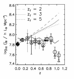
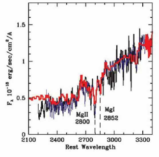
Figure 23: Left: The rest-frame blue luminosity density of ‘red sequence’ galaxies as a function of redshift from the COMBO-17 analysis of Bell et al (2004). Since such systems should brighten in the past the near-constancy of this density implies 3 times fewer red systems exist at $z\simeq$1 than locally - as expected by standard CDM models. Right: Composite spectra of red galaxies with 1.3$<z<$1.4 (blue), 1.6$<z<$1.9 (black) from the Gemini Deep Deep Survey (McCarthy et al 2004). A stellar synthesis model with age 2 Gyr is overlaid in red. The analysis suggests the most massive red galaxies with $z\simeq$5 formed with spectacular SFRs at redshifts $z\simeq$2.4-3.3.

3.7 Lecture Summary

Clearly multi-wavelength data is leading to a revolution in tracking the history of star formation in the Universe. Because of the vagaries of the stellar initial mass function, dust extinction and selection biases, we need multiple probes of star formation in galaxies.

The result of the labors of many groups is a good understanding of the comoving density of star formation since a redshift $z\simeq$3. Surprisingly, the trends observed can account with reasonable precision for the stellar mass density observed today. The implication of this result is that half the stars we see today were in place by a redshift $z\simeq$2.

What, then, are we to make of the diversity of galaxies we observe during the redshift range ($z\simeq$2-3) of maximum growth? Through detailed studies some connections are now being made between both UV-emitting Lyman break galaxies and dust-ridden sub-mm sources.

More confusion reigns in understanding the role and decline with redshift in the contribution of passively-evolving red galaxies. Some observers claim a dramatic decline in their abundance whereas others demonstrate clear evidence for the presence of a significant population of old, massive galaxies at $z\simeq$1.5. We will return to this enigma in §4.

4 Stellar Mass Assembly

4.1 Motivation

Although we may be able to account for the present stellar mass density by integrating the comoving star formation history (§3), this represents only a small step towards understanding the history of galaxy assembly. A major limitation is the fact that the star formation density averages over a range of physical situations and luminosities; we are missing a whole load of important physics. As we have seen, a single value for the stellar mass density, e.g. $\rho_{\ast}(z=2)$, is useful when considered as a global quantity (e.g. compared to an equivalent estimate at $z$=0), but it does not describe whether the observed star formation is steady or burst-like in nature, or even whether the bulk of activity within a given volume arises from a large number of feeble sources or a small number of intense objects. Such details matter if we are trying to construct a clear picture of how galaxies assemble.

Of course we could extend our study of time-dependent star formation to determine the distribution functions of star formation at various epochs (e.g. the UV continuum, $H\alpha$ or sub-mm luminosity functions), but making the integration check only at $z$=0 is second-best to measuring the assembled mass and its distribution function at various redshifts. This would allow us to directly witness the growth rate of galaxies of various masses at various times and, in some sense, is a more profound measurement, closer to theoretical predictions.

Ideally we would like to measure both baryonic and non-baryonic masses for large numbers of galaxies but, at present at least, we can only make dynamical or lensing-based total mass estimates for specific types of distant galaxy and crude estimates for the gaseous component. The bulk of the progress made in the last few years has followed attempts to measure stellar masses for large populations of galaxies. We will review their achievements in this lecture.

4.2 Methods for Estimating Galaxy Masses

What are the options available for estimating galaxy masses of any kind at intermediate to high redshift? Basically, we can think of three useful methods.

• Dynamical methods based on resolved rotation curves for recognisable disk systems (Vogt et al 1996,1997) or stellar velocity dispersions for pressure-supported spheroidals (van Dokkum & Ellis 2003, Treu et al 2005). These methods only apply for systems known or assumed a priori to have a particular form of velocity field. Interesting constraints are now available for a few hundred galaxies in the field and in clusters out to redshifts of $z\simeq$1.3. Key issues relate to biases associated with preferential selection of systems with ‘regular’ appearance and how to interpret mass dynamically-derived over a limited physical scale (c.f. Conselice et al 2005). In the absence of resolved rotation curves, sometimes emission linewidths are considered a satisfactory proxy (Newman & Davis 2000).

• Gravitational lensing offers the cleanest probe of the total mass distribution but, as a geometric method, is restricted in its application to compact, dense lenses (basically, spheroidals) occupying cosmic volumes typically half way to those probed by faint star-forming background field galaxies. In practice this means $z_{lens}<$1. Even so, by sifting through spectra of luminous red galaxies in the SDSS survey and locating cases where an emission line from a background lensed galaxy enters the spectroscopic fiber, Bolton et al (2006) have identified a new and large sample of Einstein rings enabling us to gain valuable insight into the relative distribution of dark and visible mass over 0$<z<$1.

• Stellar masses derived from near-infrared photometry represents the most popular technique in use at the current time. The idea has its origins in the recognition (Broadhurst, Ellis & Glazebrook 1992, Kauffmann & Charlot 1998) that the rest-frame $K$-band luminosity of a galaxy is less affected by recent star formation than its optical equivalent (Figure 16), and thus can act as a closer proxy to the well-established stellar population. A procedure for fitting the rest-frame optical-infrared spectral energy distribution of a distant galaxy, deriving a stellar mass/light ratio ($M/L_{K}$) and hence the stellar mass if the redshift is known, was introduced by Brinchmann & Ellis (2000). The popularity of the technique follows from the fact it can easily be applied to large catalogs of galaxies in panoramic imaging surveys and extended to very high redshift if IRAC photometry is available. The main difficulties relate to the poor precision of the method, particularly if the same photometric data is being used to estimate the redshift (Bundy et al 2006), plus degeneracies arising from poor knowledge of the past star formation history (Shapley et al 2005, van der Wel et al 2006).

For many galaxies, an important and usually neglected component is the mass locked up in both ionized and cool gas. In nearby systems amenable to study of hot ionized gas (from nebular emission lines) and its usually dominant cooler neutral component (probed by 21cm studies), as much as 20% of the baryonic mass of a luminous star-forming galaxy can be found in this form (Zwaan et al 2003). At present, it is not possible to routinely use radio techniques to reliably estimate gaseous masses of distant galaxies although approximate gas masses have been derived assuming the projected surface density of nebular emission correlates with the gas mass within some measured physical scale (Erb et al 2006).

4.3 Results: Regular Galaxies 0$<z<$1.5

Because of the simplicity of their stellar populations, velocity fields and the lack of confusing gaseous components, rather more is known about the mass assembly history of ellipticals than for spirals. Concerning ellipticals, one of the key challenges is separating the age of the stars from the age of the assembled mass.

The Fundamental Plane (FP, Dressler et al 1987, Djorgovski & Davis 1987, Bender, Burstein & Faber 1992, Jorgensen et al 1996) represents an empirical correlation between the dynamical mass (via the central stellar velocity dispersion $\sigma_{0}$), the effective radius ($R_{E}$) and light distribution (via the enclosed surface brightness $\mu_{E}$) for ellipticals, viz:

$$logR_{E}=a\,log\,\sigma_{0}\,+\,b\,\mu_{E}\,+\,c$$

For example, with $\sigma$ in km sec^-1, $R_{E}$ in kpc and $\mu_{E}$ in mags arcsec^-2 in the $B$ band, $a$=1.25, $b$=0.32, $c$=-8.970 for $h$=0.65.

These observables define an effective dynamical mass $M_{E}\propto\sigma^{2}\,R_{E}/G$ which correlates closely with that deduced from lensing (Treu et al 2006). Deviations from the local FP at a given redshift $z$ can be used to deduce the change in mass/light ratio $\Delta\,log(M/L)$.

The most comprehensive studies of the evolving FP come from two independent and consistent studies of field spheroidals to $z\simeq$1 (Treu et al 2005, van der Wel et al 2005). The evolution in mass/light ratio $\Delta\,log(M/L)$ deduced from the GOODS-N survey of Treu et al (2005) is shown in Figure 24. These authors find as little as 1-3% by stellar mass of the present-day population in massive ($>10^{11.5}M_{\odot}$) galaxies formed since $z$=1.2, whereas for low mass systems ($<10^{11}M_{\odot}$) the growth fraction is 20-40%. This result, confirmed independently by van der Wel et al (2005), is an important illustration of the mass-dependent growth in galaxies with the most massive systems shutting off earliest.

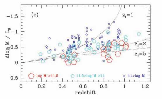
Figure 24: Change in $B$-band mass/light ratio with redshift deduced from the Keck dynamical survey of over 150 field spheroidals in GOODS-N (Treu et al 2005). The plot shows the change in mass/light ratio for galaxies of different effective dynamical masses (red: massive, cyan: intermediate, blue: low mass). Curves illustrate the change in mass/light ratio expected as a function of redshift for galaxies assembled monolithically with simply evolving stellar populations since a redshift of formation $z_{f}$. Clearly the stars in the most massive galaxies largely formed at high redshift whereas assembly continued apace in lower mass systems.

Of course, one should not confuse the age of stars, as probed by the FP, with the age of the assembled mass. van Dokkum (2005) has argued that if spheroidals preferentially merge with similar gas-poor systems (a process called ‘dry mergers’) the FP analyses could well indicate early eras of major star formation even though the bulk of the assembled mass in individual systems occurred at $z<$1 . Bell et al (2006) and Tran et al (2005) have cataloged individual cases of dry mergers in both field and cluster samples, respectively. Their occurrence is not in dispute; however, only via morphological or other measures of the global mass assembly can the role of dry mergers as a major feature of galaxy assembly be addressed.

Related insight into this problem arises from the relative distributions of baryonic and dark matter deduced from the combination of lensing and stellar dynamics for the recently-located SDSS-selected Einstein rings (Treu et al 2006, Figure 25). Although it might be thought that lensing preferentially selects the most massive and compact sources, Treu et al compare the FP of such lenses with those in the larger field sample (Fig.  25) and deduce otherwise. An important result from the study of the first set of such remarkable lenses is how well the total mass profile can be represented by an isothermal form with mass tracing light, viz:

$$\rho_{tot}=\rho\,(\frac{r}{r_{0}})^{-\gamma}$$

Even over 0$<z<$1, the mass slope $\gamma$ is constant at 2.0 to within 2% precision indicating rather precise collisional coupling of dark matter and gas.

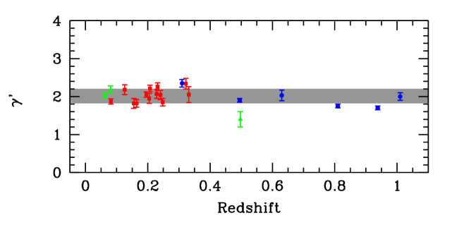
Figure 25: Distribution of the gradient $gamma$ in the total mass profile with redshift as deduced from the combination of stellar dynamics and lensing for ellipticals in the SLAC survey (Treu et al, in prepn). The remarkable constancy of the profile slope indicates massive relaxed systems were in place at $z\simeq$1 and that ‘dry merging’ cannot be a prominent feature of the assembly history of large galaxies.

Sadly, far less is known about the mass assembly history of regular spirals. The disk scaling law equivalent to the FP for ellipticals, the Tully-Fisher relation (Tully & Fisher 1977) which links rotational velocity to luminosity gives ambiguous information without additional input. Modest evolution in the TF relationship was deduced from the pioneering Keck study of $z\simeq$1 spirals by Vogt et al (1997) but this could amount to $\simeq$0.6 mag of $B$-band luminosity brightening in sources of a fixed rotational velocity to $z\simeq$1, or more enhancement if masses were reduced.

Additional variables capable of breaking the degeneracy between dynamical mass and luminosity include physical size and stellar mass. Lilly et al (1998) examined the size-luminosity relation for several hundred disks to $z\simeq$1 in a HST-classified redshift survey sample (see Sargent et al 2006 for an update) and found no significant growth for the largest systems. Conselice et al (2005) correlated stellar and dynamical masses for $\simeq$100 spirals with resolved dynamics in the context of a simple halo formulation. Although their deduced halo masses must be highly uncertain, they likewise deduced that growth must be modest since $z\simeq$1, occurring in a self-similar fashion for the baryonic and dark components.

4.4 Stellar Masses from Multi-Color Photometry

Bundy et al (2005, 2006) give a good summary and critical analysis of the now well-established practice of estimating stellar masses from multi-color optical-infrared photometry. Figure 26 gives a practical illustration of the technique where it can be seen that even for low $z$ galaxies with good photometry, the precision in mass is only $\simeq\pm$0.1-0.2 dex. In most cases, even random uncertainties are at the $\pm$0.2-0.3 dex level and systematic errors are likely to be much higher.

Figure 26: Deriving stellar masses for galaxies of known redshift via multi-color optical photometry (after Bundy et al 2006). (Left) Rest-frame spectral energy distribution of two DEEP2 galaxies of known redshift from broad-band $BRIK$ photometry with a fit deduced by fitting from a stellar synthesis library. The fit yields the most likely mass/light ratio of the observed population. (Right) Likelihood distribution of the stellar mass for the same two galaxies derived by Bayesian analysis. Dashed lines indicate the eventual range of permitted solutions.

Since analysing stellar mass functions is now a major industry in the community, it is worth spending some time considering the possible pitfalls. A significant fraction of the large datasets being used are purely photometric, with both redshifts and stellar masses being simultaneously deduced from multi-color photometry (Drory et al 2002, Bell et al 2004, Fontana et al 2004). Few large surveys have extensive spectroscopy from which to check that this procedure works.

Bundy et al (2006) address this important question in the context of their extensive DEEP2 spectroscopic sample by artificially ‘switching off’ the knowledge of the spectroscopic $z$: how does the stellar mass deduced when simultaneously deriving the photometric redshift from the same data compare with that derived when the spectroscopic value is externally input? Figure 27 illustrates that a significant component of error is one beyond that expected solely from the error in the derived redshift (as measured from the $z_{spec}$ vs. $z_{photo}$ comparison).

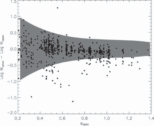
Figure 27: Error in log stellar mass when the known spectroscopic redshift is ignored (Bundy et al 2005). The shaded region defines the expected scatter in mass arising solely from that in the photometric-spectrosopic redshift comparison. Clearly in addition to this component, some catastrophic failures are evident.

A second restriction in many stellar mass determinations is the absence of any near-infrared photometry. This may seem surprising given the classic papers (Kauffmann & Charlot 1998, Brinchmann & Ellis 2000) stressed its key role. However, panoramic near-infrared imaging is much more expensive in telescope time as few observatories, until recently, had large format infrared cameras. Inevitably, some groups have attempted to get by without the near-infrared data.

Figure 28 illustrates how the precision degrades when the $K$ band data is dropped in the stellar mass fit (Bundy et al 2006). Although the systematic error is contained, the noise increases significantly for redshifts $z>$0.7 where the optical photometry fails to adequately sample the older, lower mass stars.

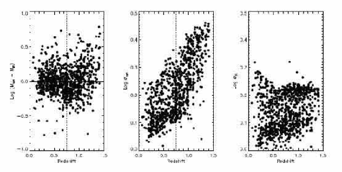
Figure 28: Effect of deriving stellar masses from optical photometry alone (Bundy et al 2006). (Left) Difference in masses derived using $BRIK$ and $BRI$ photometry. (Center) Distribution of uncertainties deduced from Bayesian fitting for the $BRI$ fits. (Right) as center for the $BRIK$ fitting. Although the systematic offset is small, the uncertainty in deduced stellar mass increases dramatically for galaxies with $z>$0.7.

Shapley et al (2005) explore a further uncertainty, which is particularly germane to the analysis of their $z\simeq$2 sources. Using IRAC to represent the rest-frame infrared at these redshifts, they consider the role that recent bursts of star formation might have on the deduced stellar masses. Although bursts predominantly affect short-wavelength luminosities, one might imagine little effect at the longer wavelengths (c.f. Kauffmann & Charlot 1998). Shapley et al consider a wider range of star formation histories and show that the derived stellar mass depends less strongly on the long wavelength luminosity $L$ (4.5$\mu$m) than expected. The scatter is consistent with variations in mass/light ratios of $\times$15 (Figure 29). The strong correlation between mass and optical-infrared color emphasizes the importance of secondary activity.

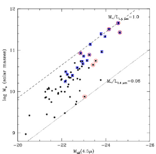
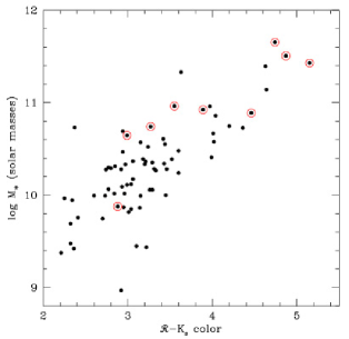
Figure 29: Left: Stellar masses versus observed IRAC 4.5$\mu$m luminosities for the sample of $z\simeq$2 galaxies studied by Shapley et al (2005). Allowing a wide range of star formation histories illustrates a weaker dependence of mass on long wavelength luminosity than seen in earlier tests at lower redshift based on simpler star formation histories. The range in rest-frame 1.6$\mu$m mass/light ratio is $\simeq\times$15. (Right) The existence of a fairly tight correlation between mass and $R-K$ color demonstrates the importance of considering secondary bursts of star formation in deriving stellar masses.

4.5 Results: Stellar Mass Functions 0$<z<$1.5

Noting the above uncertainties, we now turn to results compiled from the stellar mass distributions of galaxies undertaken in both spectroscopic and photometric surveys. A recent discussion of the various results can be found in Bundy et al (2006).

Brinchmann & Ellis (2000) were the first to address the global evolution of stellar mass in this redshift range using a morphological sample of 350 galaxies with spectroscopic redshifts and infrared photometry. The small sample did not permit consideration of detailed stellar mass functions, but the integrated mass density was partitioned in 3 redshift bins for spheroidals, spirals and irregulars. Surprisingly little growth was seen in the overall mass density from $z\simeq$1 to today; the strongest evolutionary signal seen is a redistribution of mass amongst the morphologies dominated by a declining mass density in irregulars with time.

The ratio of the galactic stellar mass $M_{star}$ to the current star formation rate $SFR$, e.g. as deduced spectroscopically or from the rest-frame optical colors, is sometimes termed the specific star formation rate, $R$. This quantity allows us to address the question of whether galaxies have been forming stars for a significant fraction of the Hubble time, at a rate commensurate with explaining their assembled mass. A low value for $R$ implies a quiescent object whose growth has largely ended; the mean stellar age is quite large. A high value of $R$ implies an active object which has assembled recently. A frequently-used alternative is the ‘doubling time’ - that period over which, at the current SFR, the observed stellar mass would double. This time would be quite short for active objects.

Cowie et al (1996), Brinchmann & Ellis (2000), and most recently Juneau et al (2005), found a surprising trend whereby most massive galaxies over $z\simeq$0.5-1.5 are quiescent, having presumably formed their stars well before $z\simeq$2, whereas low mass galaxies remain surprisingly active. The term ‘downsizing’ - a signature of continued growth in lower mass galaxies after that in the high mass galaxies has been completed - was first coined by Cowie et al (1996) and has been used rather loosely in the recent literature to imply any signature of anti-hierarchical activity. In particular, it is important to distinguish between downsizing in star formation activity, which presumably represents some physical process that permits continued star formation in lower mass systems when that in massive galaxies has concluded, from downsizing in mass assembly, a truly ‘anti-hierarchical’ process whereby new mass is being added to lower mass galaxies at later times (see discussion in Bundy et al 2006).

Before trying to understanding in more detail what causes this mass-dependent star formation, it is worth returning to the issue of dry mergers raised in $\S 4.3$. A ‘downsizing’ signature was also seen in the growth of spheroidal galaxies as analysed by their location on the evolving Fundamental Plane (Treu et al 2005, van der Wel et al 2005). However, van Dokkum (2005) argued that while this may reflect older stars in the more massive galaxies, the assembled mass may still be young if merging preferentially occurs between quiescent objects. The only way to test this hypothesis is to directly measure the growth rate in spheroidal systems.

Using the deeper and more extensive sample of galaxies available in the GOODS fields, Bundy et al (2005) produced type-dependent stellar mass functions (Figure 30). Here, for the first time, one can see the morphological evolution detected by Brinchmann & Ellis largely arises via the transformation of intermediate mass ($\simeq$5. 10¹⁰ - 2.10${}^{11}M_{\odot}$) irregulars and spirals into spheroidals. If merging is responsible for this transformation, it is predominantly occurring between gas-rich and active systems even at the very highest masses. The bulk of the evolution below $z\simeq$1 is simply a redistribution of star formation activity, perhaps as a result of mergers or feedback processes.

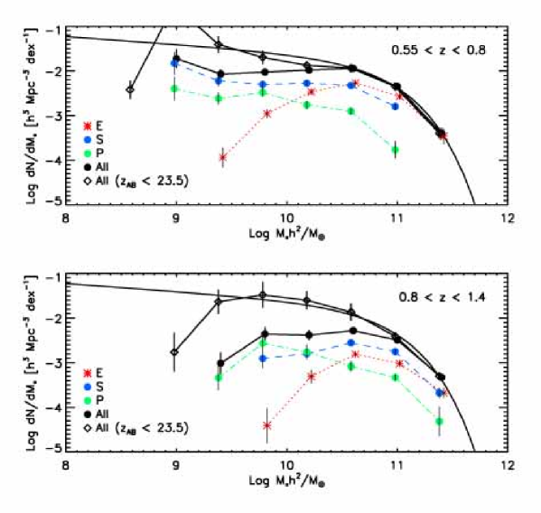
Figure 30: Stellar mass function arranged by morphology in two redshift bins from the analysis of Bundy et al (2005) for $h$=1. The solid curve in both plots represents the present day mass function from the 2dF survey (Cole et al 2003). Type-dependent mass functions are color-coded with black representing the total. The solid line connecting the filled black circles represents the sample with spectroscopic redshifts, the dotted line connecting the open black diamonds includes masses derived from sources with photometric redshifts. The vertical dashed lines represent completeness limits for all types.

Interestingly, in Figure 30 there is almost no change in the total mass function with time above 5. 10${}^{10}M_{\odot}$, suggesting little growth in the mass spheroidals that dominate the high mass end. However, it worth remembering that the two GOODS fields are limited in size (0.1 deg²) and suffer from cosmic variance at the 20% level at high redshift increasing to 60% at low redshift (Bundy et al 2005).

Stellar mass functions for a much larger sample of field galaxies of known redshift have been analyzed by Bundy et al (2006) utilizing the combination of extensive spectroscopy and Palomar $K$-band imaging in four DEEP2 fields (totalling 1.5 deg²). This sample has the benefit of being much less affected by cosmic variance although, as there is no complete coverage with HST, morphological classifications are not possible. Color bimodality has been analyzed in the DEEP2 sample (Weiner et al 2005) and Bundy et al use the rest-frame $U-B$ color and spectroscopic [O II] equivalent width to separate quiescent and active galaxies.

Figure 31 shows a direct comparison of the integrated stellar mass functions from this large survey alongside other, less extensive surveys, most of which are based only on photometric redshifts. Although each is variance limited in different ways, one is struck again by the quite modest changes in the abundance of massive galaxies since $z\simeq$1.

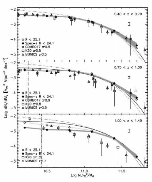
Figure 31: The evolving stellar mass function from the comparison of Bundy et al (2006).

Next we consider (Figure 32) the stellar mass functions for the quiescent and active star-forming galaxies independently, partitioned according to the rest-frame $U-B$ color. The surprising result here is the existence of a threshold or quenching mass, $M_{Q}$ above which there are no active systems. This is implied independently in Figure 30 where, within the redshift bin $0.55<z<0.8$, there are no spirals or irregulars with mass $>10^{11}M_{\odot}$. Interestingly, there is also a modest downward transition in $M_{Q}$ with time.

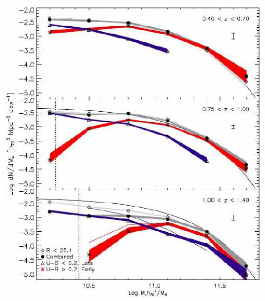
Figure 32: The evolving stellar mass function split into quiescent (red) and active (blue) sources from the survey of Bundy et al (2006). Uncertainties arising from counting statistics and errors in the stellar masses are indicated by the associated shading. The thin solid line represents the local 2dF function (Cole et al 2003) and the dark and light grey regions represent total mass functions using only spectroscopic and including photometric redshifts respectively.

A remarkably consistent picture emerges from these studies. Over the redshift range 0$<z<$1.5, the stellar mass function has changed very little at the high mass end. Substantial growth, in terms of a mass doubling on $\simeq$5-8 Gyr timescale, is only possible for galaxies with stellar masses below 10${}^{10}\,M_{\odot}$. Above this mass, the basic evolutionary signal is a quenching of star formation in well-established systems. This quenching progresses toward lower mass systems at later times, consistent with the mass-dependent trends seen in the ages of stellar populations in the quiescent spheroidals.

The physical origin of the quenching of star formation, the fundamental origin of the various downsizing signals, is unclear. Although the merger-induced production of active galactic nuclei may lead to the temporary expulsion and heating of the gaseous halos that surround galaxies (Springel et al 2005, Croton et al 2006), key tests of this hypothesis include sustaining the quenching, the weak environmental dependence of the observational trends and the surprisingly clear redshift dependence of the effect (Figure 32).

4.6 Results: Stellar Mass Functions z$>$1.5

With current facilities, the stellar mass data beyond $z\simeq$1.5 generally probes only the higher mass end of the distribution and relies on photometric rather than spectroscopic data. Nonetheless, the results emerging have received as much attention as those at lower redshift. Unlike the complexities of understanding downsizing and the redistribution of mass and morphology in the $z<$1 data, the basic question at stake here is simply whether the abundance of massive $z\simeq$2 galaxies is larger than expected in the standard model.

Testing the decline with redshift in the comoving abundance of, say, systems with stellar mass greater than 10${}^{11}\,M_{\odot}$, expected in $\Lambda\,CDM$ has been a frustrating story for the observers for two reasons. Firstly, the most massive systems are rare and clustered, and so determining reliable density estimates beyond $z\simeq$1.5 has required panoramic deep infrared data which has only recently arrived. For a review of the early observational efforts see Benson, Ellis & Menanteau (2002)

Secondly, there has been considerable confusion in the theoretical literature on the expected rate of decline in $>10^{11}\,M_{\odot}$ systems. Early predictions (Kauffmann, Charlot & White 1996) claimed a 3-fold decline in the comoving abundance to $z\simeq$1 in apparent agreement with the large photometric sample analyzed by Bell et al (2004). However, careful comparisons of independent semi-analytical predictions (Kauffmann et al 1999, Cole et al 2000) reveal substantial differences (by an order of magnitude for the same world model) in the rate of decline even to $z\simeq$1 (Benson, Ellis & Menanteau 2002). In reality, the predictions depend on many parameters where differences can have a large effect for the region of the mass function where the slope $dN\,/\,dM$ is steep.

Dickinson et al (2003) undertook a pioneering study to evaluate the growth of stellar mass with photometric redshift using deep $H<$26.5 NICMOS data in the Hubble Deep Field North. Although a tiny field (5 arcmin²), the work was the first to demonstrate the existence of $10^{11}\,M_{\odot}$ galaxies at $z\simeq$1.5-2 as well as the challenges of estimating reliable abundances. A similar HDF-S analysis was undertaken by Rudnick et al (2003).

A more representative area of 4$\times$30 arcmin was probed spectroscopically in the Gemini Deep Deep Survey (Glazebrook et al 2004), albeit to a much shallower depth. These authors claimed a ‘surprising’ abundance of $10^{11}\,M_{\odot}$ systems to $z\simeq$2. Although an absolute comparison of the abundances with semi-analytical predictions is not likely to be illuminating for the reasons mentioned above, the redshift-dependent mass growth rate over 1$<z<$2, derived empirically from both the stellar masses and the integrated star formation rate, seems much slower than expected in the semi-analytical models (Granato et al 2000). Of particular interest is the fact that the mass growth rate seems not depend strongly on the mass range in question in apparent disagreement with the model predictions (Figure 33).

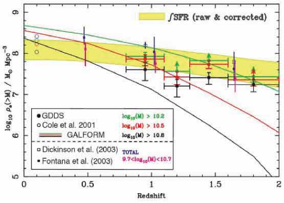
Figure 33: The mass assembly history derived from stellar masses in the Gemini Deep Deep spectroscopic survey (Glazebrook et al 2004). Colored data points refer to observed cumulative densities $\rho\,(\,>M)$ for various mass ranges and the green shaded region to estimates derived from the integrated star formation history. The colored lines refer to predicted growth rates according to the GALFORM semi-analytic models.

Although many of the observers associated with the Gemini Deep Deep Survey have claimed the abundance and slow growth rate of massive galaxies over 1.5$<z<$2 poses a crisis for the standard model, alongside the puzzling ‘anti-hierarchical’ behavior observed for $z<$1.5, the plain fact is that there is considerable uncertainty in the semi-analytical predictions.

4.7 Quiescent Galaxies with 2$<z<$3

Finally, it is illustrative to consider the dramatic effect that infrared data from panoramic ground-based cameras and the Spitzer Space Telescope is having, not only on our knowledge of the distribution of stellar masses at high redshift, but also how stellar mass is distributed among quiescent and star-forming populations. Until recently, there was widespread belief that the bulk of the star formation in this era, and probably a significant fraction of the stellar mass, lay in the Lyman break population. By contrast, van Dokkum et al (2006) have examined the rest-frame $U-V$ colors of a sample of 300 $>10^{11}\,M_{\odot}$ galaxies with 2$<z_{photo}<3$ (Figure 34) and claim almost 80% are quiescent. The definition of ‘quiescent’ here is somewhat important to get correct, given it now emerges that many of the originally-selected distant red galaxies with $J-K>$2.3 (§2.6) turn out to have quite respectable star formation rates. Infrared spectroscopy sensitive to $H\alpha$ emission and the 4000Å break is making great strides in clarifying this question (Kriek et al 2006).

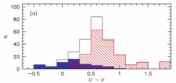
Figure 34: The distribution of rest-frame U-V color for a Spitzer-selected sample of $2<z<$3 galaxies with stellar masses $>10^{11}\,M_{\odot}$ from the analysis of van Dokkum et al (2006). Almost 80% of this sample in a quiescent state consistent with having completed the bulk of their assembly.

4.8 Lecture Summary

In this lecture we have demonstrated important new techniques for estimating the stellar masses of all types of galaxies to impressive high redshift ($z\simeq$3). The reliability of these techniques is improved greatly by having spectroscopic, rather than photometric, redshifts and, for $z>0.7$, by the addition of infrared photometry. These techniques augment and extend more precise measures available for restricted classes of galaxies - such as the Fundamental Plane for pressure-supported spheroidals, and the Tully-Fisher relationship for rotationally-supported disks.

These various probes point to a self-consistent, but puzzling, description of mass assembly since $z\simeq$1.5. During this era, massive galaxies have hardly grown at all - most of the star formation and rapid growth is occurring in systems whose masses are less than $10^{10}\,M_{\odot}$. Remarkably, the star formation appears to be quenched above a certain threshold mass whose value, in turn, is declining with time.

Energetic sources such as supernovae or active nuclei may be responsible for this ‘downsizing’ signature but further work is needed to verify both the weak environmental trends seen in the observations and the redshift-dependent trends in the threshold mass.

Beyond $z\simeq$1.5, the number and distribution of massive ($>10^{11}\,M_{\odot}$ galaxies has led to some surprises. Although the sheer abundance may not be a problem for contemporary models, the fact that so many have apparently completed their star formation is more challenging and consistent with the slow growth rate observed at later times. The observational situation is rapidly developing but consistent with the presence of a surprisingly abundant and mature population of massive galaxies by $z\simeq$3.

5 Witnessing the End of Cosmic Reionization

5.1 Introduction - Some Weighty Questions

We now turn to the exciting and rapidly developing area of understanding cosmic reionization. This event, which marks the end of the so-called ‘Dark Ages’ when the intergalactic medium became transparent to ultraviolet photons, was a landmark in cosmic history. In some ways the event might be considered as important as the epoch of recombination which isolates the formation of the hydrogen atom, or the asssociated surface of last scattering when photons and baryonic matter decouple. In the case of the era of cosmic reionization, although we cannot yet be sure, many believe we are isolating that period when the first sources had sufficient output to contribute to the energy balance of the intergalactic medium. Even though some early luminous forerunners might be present, the epoch of reionization can be directly connected with cosmic dawn for starlight.

It seems an impossible task to give an authoritative observational account of how to probe this era. So many issues are complete imponderables! When did reionization occur? Was it a gradual event made possible by a complex time sequence of sources, or was there a spectacular synchronized moment? Can we conceive of an initial event, followed by recombination and a second phase?

What were the sources responsible? History has shown the naivety of astronomers in assuming a single population to be responsible for various phenomena - usually some complex combination is the answer. And, perhaps most ambitiously, what is the precise process by which photons escape the sources and create ionized regions?

Four independent observational methods are helpful in constraining the redshift range where we might search for answers to the above questions. In this lecture, we will explore how these work and the current (and rapidly changing) constraints they offer. These are:

• Evolution in the optical depth of Lyman series absorption lines in high redshift quasars (Fan et al 2006a,b). Although QSOs are only found to redshifts of $z\simeq$6.5, high quality spectroscopic data gives us a glimpse of a potential change in the degree of neutrality of the IGM beyond $z\simeq$5.5 such as might be expected if reionization was just ending at that epoch.

• The ubiquity of metal absorption lines in the IGM as probed again by various spectra of the highest redshift QSOs. Carbon, in particular, is only produced in stellar nuclei and its presence in all sightlines to $z\simeq$5-6 (Songaila 2004) is highly indicative of a widespread process of earlier enrichment from the first generation of supernovae.

• The large angular scale power in the temperature - polarization cross-correlation function seen in the microwave background (Kogut et al 2003, Spergel et al 2006). This signal is produced by electron scattering foreground to the CMB. Depending on models of large scale structure, the optical depth of scattering gives some indication of the redshift range where the ionized particles lie.

• The stellar mass density in assembled sources at redshifts $z\simeq$5-6, about 1 billion years after the Big Bang, as probed by the remarkable combination of HST and Spitzer (Stark & Ellis 2005, Stark et al 2006a, Yan et al 2006, Eyles et al 2006). A census of the mass in stars must be the integral of past activity which can be compared with that necessary to reionize the Universe.

5.2 The Gunn-Peterson Test and SDSS QSOs

In a remarkable paper, long before QSOs were located at redshifts beyond 2.5, James Gunn and Bruce Peterson realized (Gunn & Peterson 1965) that the absence of broad troughs of hydrogen absorption in the spectra of QSOs must indicate intergalactic hydrogen is ionized. They postulated a future test whereby the spectra of QSOs of successively higher redshift would be scrutinized to locate that epoch when the IGM was neutral.

For an optical spectrum, redshifted to reveal that portion of the rest-frame UV shortward of the Lyman $\alpha$ emission line of the QSO itself ($\lambda$ 1216 Å ), the relative transmission $T$ is defined as

$$T=f(\lambda)\,/\,f_{cont}$$

where $f_{cont}$ represents the continuum radiation from the QSOs. The transmission is reduced by Lyman $\alpha$ absorption in any foreground (lower redshift) clouds of neutral hydrogen whose Gunn-Peterson opacity is then

$$\tau_{GP}=-ln\,T$$

The first ‘complete troughs’ in the absorption line spectra of distant QSO were presented by Becker et al (2001) and Djorgovski et al (2001) and a more comprehensive sampling of 11 SDSS QSOs was presented by Fan et al (2003). Recently, an analysis of 19 5.74$<z<$6.42 QSOs was presented by Fan et al (2006b).

Figure 35 illustrates how absorption structures along the same line of sight can be independently probed using Lyman $\alpha$ and higher order lines such as Lyman $\beta$.

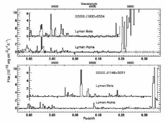
Figure 35: The absorption line spectrum of two SDSS QSOs from the recent study of Fan et al (2006b). Here the structures in the Lyman series absorption lines $\alpha$ and $\beta$ have been aligned in redshift space thereby improving the signal to noise along a given sightline. The effects of cosmic variance can clearly be seen by comparing the structures seen along the two sightlines.

To understand how this is effective, in a uniform medium $\tau_{GP}$ is related to the abundance of absorbing neutral hydrogen atoms by the following expression:

$$\tau_{GP}=\frac{\pi e^{2}}{m_{e}c}\,f_{\alpha}\,\lambda_{\alpha}\,H^{-1}(z)\,n_{HI}$$

where $f$ is the oscillator strength of the Lyman $\alpha$ line, $H$ is the redshift-dependent Hubble parameter and $n_{HI}$ is the neutral number density.

Numerically, this becomes

$$\tau_{GP}=1.8\,10^{5}h^{-1}\,\Omega_{m}^{-\frac{1}{2}}\,\frac{\Omega_{b}h^{2}}{0.02}\,(\frac{1\,+\,z}{7})^{3/2}\,\frac{n_{HI}}{n_{H}}$$

where $x_{HI}=(\frac{1\,+\,z}{7})^{3/2}\,\frac{n_{HI}}{n_{H}}$ is then the neutral fraction.

Inspection of this equation is quite revealing. Firstly, even a tiny neutral fraction, $x_{HI}\sim 10^{-4}$, would give a very deep, seemingly complete GP trough; for reference $x_{HI}\simeq 10^{-5}$ today. So clearly the test is not a very sensitive one in absolute terms.

Secondly, since $\tau_{GP}\,\propto\,f\,\lambda$, for the same $n_{H}$, the optical depth in the higher order Lyman $\beta$ and $\gamma$ lines would be $\simeq$6 and 18 times smaller respectively.

In practice, the above relations are greatly complicated by any clumpiness in the medium. This affects our ability to make direct inferences on $x_{HI}$ as well as to combine the various Lyman lines into a single test.

Instead, workers have examine the relative distribution of $\tau_{GP}$ with redshift independently from the various Lyman series absorption statistics. An increase in $\tau_{GP}$ with redshift could just be a natural thickening of the Lyman absorption forest and, given its weak connection with $x_{HI}$, not imply anything profound about cosmic reionization. However, if it can be shown empirically that the various diagnostics show a discontinuity in the $x_{HI}$-redshift trends, conceivably we are approaching the neutral era.

Figure 36 shows that for $z<$5.5, $\tau\propto(\frac{1+z}{5})^{4.3}$ for both the Ly$\alpha$ and Ly$\beta$ forests to reasonable precision. However, beyond $z\simeq$5.5, both redshift trends are much steeper, $\propto(1+z)^{11}$. The dispersion around the trends also increases significantly at higher redshift. Taken together, both results suggest a qualitative change in nature of the IGM beyond $z\simeq$5.5 (but for an alternative explanation see Becker et al 2006).

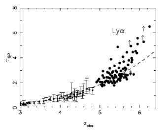
Figure 36: Evolution in the Gunn-Peterson optical depth, $\tau$, for both the Lyman $\alpha$ (left) and $\beta$ (right) forests from the distant SDSS QSO analysis of Fan et al (2006. The dotted lines represent fits to the data for $z_{abs}<$5.5, beyond which there is evidence in both species for an upturn in the opacity of the intergalactic medium.

Fan et al (2006a,b) discuss several further probes of the nature of the IGM at $z\simeq$6. One relates to the proximity effect - the region around each QSO where it is clear from the spectrum that the IGM is being ionized by the QSO itself. Although this region is excluded in the analyses above, the extent of this region contains valuable information on the nature of the IGM. It appears that the radius of the region affected, $R$ is less at higher redshift according to $R\propto[(1\,+\,z)\,x_{HI}]^{-1/3}$ suggesting that the most distant QSOs in the sample ($z\simeq$6.5) lie in a IGM whose neutral fraction is $\simeq$14 times higher than those at $z\simeq$5.7.

Another valuable measure is how the regions of complete absorption, the so-called ‘dark gaps’ in the spectrum where transmission is effectively zero, are distributed. Fan et al define a ‘gap’ as a contiguous region in redshift space where $\tau>$3.5. The distribution of gaps contains some information on the topology of reionization. We would expect regions of high transmission to be associated with large HII regions, centered on luminous star-forming sources. The dark gaps increase in extent from $\simeq$10 to 80 comoving Mpc over the redshift range samples suggesting the IGM is still not neutral at $z\simeq$6.5. Although the Gunn-Peterson and gap statistics make similar statements about reionization, suggesting the neutral fraction at $z\simeq$6.2 is 1-4%, Fan et al consider that beyond $z\simeq$6.5, gap statistics will become a more powerful probe. This is because the redshift distribution of those few spectroscopic pixels where the transmission is non-zero will become the only effective signal.

5.3 Metallicity of the High Redshift IGM

A second measure of the redshift range of early star formation is contained in the properties of the CIV forest observed in the spectra of high redshift QSOs (Songaila 2005, 2006). Carbon is only produced in stellar nuclei (it is not produced in the hot Big Bang) and so the ubiquity of CIV along many sightlines to $z\simeq$5-6 QSOs is a powerful argument for early enrichment.

CIV was seen in the Ly$\alpha$ forest in 1995 (Cowie et al 1995) with N(CIV)/N(HI) $\sim$10^-2 to 10^-3. However, it was subsequently seen in even the weakest Ly$\alpha$ systems (Ellison et al 2000). This is a particularly powerful point since it argues that enrichment is not confined to localized regions of high column density but is generic to the intergalactic medium as a whole (Figure 37)

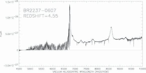
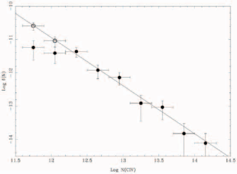
Figure 37: (Left) Keck ESI absorption line spectrum of the z=4.5 QSO BR2237-0607 from the study of Songaila (2005). A sparsely populated CIV forest from 7500-8500Å accompanies the dense Ly$\alpha$ forest seen below 6800 Å . (Right) Distribution of column densities of CIV absorbers per unit redshift interval in Q1422+231 from the survey of Ellison et al (2000).

A quantitative interpretation of the CIV abundance, in terms of how much early star formation occurred earlier than the highest redshift probed, relies on locating a ‘floor’ in the abundance-redshift relation. Unfortunately, the actual observed trend, measured via the contribution of the ion to the mass density $\Omega(CIV)$ from $z\simeq$5 to 2, does not seem to behave in the manner expected. For example, there is no strong rise in the CIV abundance to lower redshift despite the obvious continued star formation that occurred within these epochs (Songaila 2006, Figure 38). This is a major puzzle (c.f. Oppenheimer et al 2006).

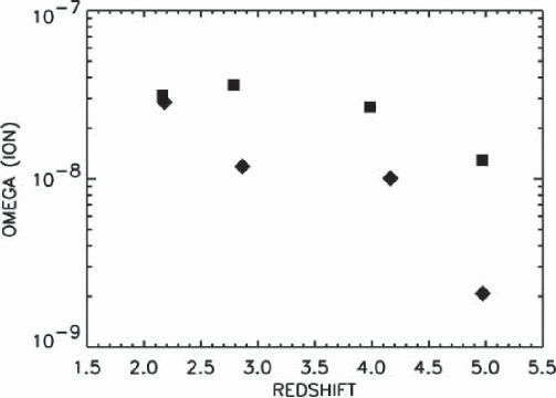
Figure 38: Modest evolution in the contribution of intergalactic CIV and SIV over 2$<z<$5 as measured in terms of the ionic contribution to the mass density, $\Omega$ (Songaila 2005).

5.4 Linear Polarization in the WMAP Data

In 2003, the WMAP team (Kogut et al 2003) presented the temperature-polarization cross angular power spectrum from the first year’s data and located a 4$\sigma$ non-zero signal at very low multipoles ($l<$8) which they interpreted in terms of foreground electron scattering of microwave background photons with an optical depth $\tau_{e}=0.17\pm 0.04$ corresponding to ionized structures at $z_{reion}\simeq$20 (Figure 39a). The inferred redshift range depends sensitively on the history of the reionization process. Bennett et al (2003) argued that if reionization occurred instantaneously it corresponds to a redshift $z_{reion}\simeq 17\pm 5$, whereas adopting a more reasonable Press-Schechter formalism and an illustrative cooling and enrichment model, Fukugita & Kawasaki (2003) demonstrated that the same signal can be interpreted with a delayed reionization occurring at $z_{reion}\simeq$9-10.

Just before the Saas-Fee lectures, the long-awaited third year WMAP data was published (Spergel et al 2006). A refined analysis significantly lowered both the normalization of the dark matter power spectrum to $\sigma_{8}=0.74\pm 0.05$, and the optical depth to electron scattering to $\tau_{e}=0.09\pm 0.03$. The same model of instantaneous reionization reduces the corresponding redshift to $z_{reion}=11\pm 3(2\sigma)$ - a significant shift from the 1 year data.

To illustrate the uncertainties, Spergel et al introduce a more realistic history of reionization via the ionization fraction $x_{e}$. Suppose above $z_{reion}$, $x_{e}\equiv 0$ and below $z$=7, $x_{e}\equiv 1$. Then suppose $z_{reion}$ is defined as that intermediate point when $x_{e}=x_{e}^{0}$ for 7$<z<z_{reion}$. Figure 39b illustrates the remarkable insensitivity of $z_{reion}$ to the adopted value of $x_{e}^{0}$ for $x_{e}^{0}<$0.5. Despite improved data, the redshift range implied by the WMAP data spans the full range 10$<z<$20.

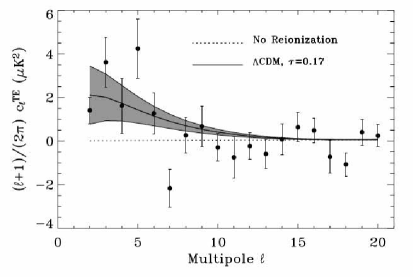
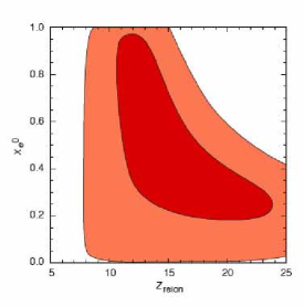
Figure 39: (Left) The 4$\sigma$ detection of reionization via an excess signal at large scales in the angular cross correlation power spectrum of the temperature and polarization data in the first year WMAP data (Kogut et al 2003). (Right) Constraints on the redshift of reionization, $z_{reion}$, from the third year WMAP data (Spergel et al 2006). The contours illustrate how the $z_{reion}$ inferred from the lowered optical depth depends on the history of the ionized fraction $x_{e}(z)$, see text for details.

5.5 Stellar Mass Density at $z\simeq$5-6

Neither the Gunn-Peterson test nor the WMAP polarization data necessarily demonstrate that reionization was caused by early star-forming sources; both only provide constraints on when the intergalactic medium was first reionized. The CIV test is a valuable complement since it provides a measure of early enrichment which can only come from star-forming sources. Unfortunately, powerful though the ubiquitous presence of CIV is in this context, as we have seen, quantitative constraints are hard to derive. We thus seek a further constraint on the amount of early star formation that might have occurred.

In Lecture 4 we introduced the techniques astronomers are now using to derive stellar masses for distant galaxies. Although the techniques remain approximate, it must follow that the stellar mass density at a given epoch represents the integral over time and volume of the past star formation. Indeed, we already saw a successful application of this in reconciling past star formation with the local stellar mass density observed by 2dF (Figure 21). Specifically, at a particular redshift, $z$

$$M_{\ast}=\int_{\infty}^{z}\rho_{\ast}(z)\,dV(z)$$

Using the techniques described in Lecture 4, stellar mass estimates have become available for some very high redshift galaxies detected by Spitzer (Eyles et al 2005, Mobasher et al 2005, Yan et al 2005). For the most luminous Lyman ‘dropouts’, these estimates are quite substantial, some exceeding $10^{11}\,M_{\odot}$ implying much earlier activity. Recently, several groups (Stark et al 2006a, Yan et al 2006, Eyles et al 2006) have been motivated to provide the first crude estimates on the volume averaged stellar mass density at these early epochs. Part of this motivation is to check whether the massive galaxies seen at such high redshift can be reconciled with hierarchical theory, but as Stark & Ellis (2005) proposed, the established stellar mass can also be used to probe earlier star formation and its likely impact upon cosmic reionization.

A very relevant question is whether the observed mass density at $z\simeq$5-6 is greater than can be accounted for by the observed previous star formation history. We will review the rather uncertain data on the star formation density $\rho_{\ast}(z)$ beyond $z\simeq$6 in the next Lecture. However, Stark et al (2006a) find that even taking a reasonably optimistic measure of $\rho_{\ast}(z)$ from recent compilations by Bouwens et al (2006) and Bunker et al (2006), it is hard to account for the stellar mass density at $z\simeq$5 (Figure 40).

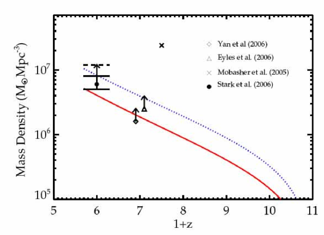
Figure 40: A comparison of the assembly history of stellar mass inferred from the observed decline in star formation history to $z\simeq$10 (solid line) with extant data on the stellar mass density at $z\simeq$5 and 6 (data points from Stark et al 2006a, Yan et al 2006, Eyles et al 2006). Different estimates at a given redshift represent lower limits based on spectroscopically-confirmed and photometric redshift samples. The red line shows the growth in stellar mass expected from the presently-observed luminous star forming galaxies; a shortfall is observed. The blue dotted line shows the improvement possible when a dominant component of high z lower luminosity systems is included.

There are currently two major limitations in this comparison. First, most of the v- and i-drops are located photometrically; even a small degree of contamination from lower redshift galaxies could upward bias the stellar mass density. On the other hand only star-forming galaxies are located by the Lyman break technique so this bias could easily be offset if there are systems in a quiescent state as evidenced by the prominent Balmer breaks seen in many of the Spitzer-detected sources (Eyles et al 2005, 2006). This limitation will ultimately be overcome with more careful selection methods and deeper spectroscopy. Secondly, and more profoundly, the precision of the stellar masses may not be up to this comparison. Much has to be assumed about the nature of the stellar populations involved which may, quite reasonably, be somewhat different from those studied locally. The discrepancy noted by Stark et al is only a factor of $\times$2-3, possibly within the range of uncertainty.

Regardless, if this mismatch is reinforced by better data, the implications are very interesting in the context of reionization. It could mean early star-forming systems are extincted, lie beyond $z\simeq$10 where current searches end, or perhaps most likely that early star formation is dominated by lower luminosity systems (Figure 40). By refining this technique and using diagnostics such as the strength of the tell-tale Balmer break, it may ultimately be possible to age-date the earlier activity and compare its efficacy with that required to reionize the Universe.

5.6 Lecture Summary

In this lecture we have introduced four very different and independent probes of cosmic reionization, each of which suggests star formation activity may extend well into the redshift range 6$\,<z<\,$20. Two of these probes rely on a contribution from early star formation (the metallicity of the intergalactic medium and the assembled stellar mass density at $z\simeq$5-6).

The earliest result was the presence of neutral hydrogen troughs in the spectra of distant QSOs. Although the arguments for reionization ending at $z\simeq$6 seem compelling at first sight, they ultimately rely on an empirically-deduced transition in the changes in the opacity of the Ly$\alpha$ and Ly$\beta$ line below and above $z\simeq$5.5.

The second result - the ubiquity of carbon in even the weakest absorbing clouds at $z\simeq$5 is firm evidence for early star formation. However, it seems hard to locate the high redshift ‘abundance floor’ and hence to quantify whether this early activity is sufficient for reionization. Indeed, a major puzzle is the lack of growth in the carbon abundance over the redshift range where galaxies are assembling the bulk of their stars.

The WMAP polarizations results have received the most attention, mainly because the first year data indicated a surprisingly large optical depth and a high redshift for reionization. However, there were some technical limitations in the original analysis and it now seems clear that the constraints on the redshift range when the foreground polarization is produced are not very tight.

Finally, an emerging and very promising technique is simply the census of early star formation activity as probed by the stellar masses (and ages) of the most luminous dropouts at $z\simeq$5-6. Although significant uncertaintes remain, the prospects for improving these constraints are good and, at this moment, it seems there must have been quite a significant amount of early ($z>$6) star formation activity, quite possibly in low luminosity precursors.

6 Into the Dark Ages: Lyman Dropouts

6.1 Motivation

Surveys of galaxies at and beyond a redshift $z\simeq$6 represent the current observational frontier. We are motivated to search to conduct a census of the earliest galaxies seen 1 Gyr after the Big Bang as well as to evaluate the contribution of early star formation to cosmic reionization. Although impressive future facilities such as the next generation of extremely large telescope and the James Webb Space Telescope (Gardner et al 2006) are destined to address these issues in considerable detail, any information we can glean on the abundance, luminosity and characteristics of distant sources will assist in planning their effective use.

In this lecture and the next, we will review the current optical and near-infrared techniques for surveying this largely uncharted region. They include

• Lyman dropouts: photometric searches based on locating the rest-frame ultraviolet continuum of star-forming sources introduced in Lecture 3. The key issue here is reducing contamination from foreground sources since most sources selected via this technique are too faint for confirmatory spectroscopy.

• Lyman alpha emitters: spectroscopic or narrow-band searches for sources with intense Ly$\alpha$ emission. As the line is resonantly-scattered by neutral hydrogen its profile and strength gives additional information on the state of the high redshift intergalactic medium.

• Strong gravitational lensing: by coupling both above techniques with the magnification afforded by lensing clusters, it is possible to search for lower luminosity sources at high redshift. Since the magnified areas are small, the technique is only advantageous if the luminosity function has a steep faint end slope.

For the Lyman dropouts discussed here, as introduced in the last lecture, there is an increasingly important role played by the Spitzer Space Telescope in estimating stellar masses and earlier star formation histories.

The key questions we will address in this lecture focus on the (somewhat controversial) conclusions drawn from the analyses of Lyman dropouts thus far, namely:

1. How effective are the various high $z$ selection methods? The characteristic luminosity $L^{\ast}$ at $z\simeq$6 corresponds to $i_{AB}\simeq$26 where spectroscopic samples are inevitably biased to those with prominent Ly$\alpha$ emission. Accordingly there is great reliance on photometric redshifts and a real danger of substantial contamination by foreground red galaxies and Galactic cool stars.

2. Is there a decline in the UV luminosity density, $\rho_{UV}$, over the range 3$<z<$6? The early results were in some disagreement. Key issues relate to the degree of foreground contamination and cosmic variance in the very small deep fields being examined.

3. Is the observed UV density, $\rho_{UV}$, at $z\simeq$6 sufficient to account for reionization? The answer depends on the contribution from the faint end of the luminosity function and whether the UV continuum slope is steeper than predicted for a normal solar-metallicity population.

4. Significant stellar masses have been determined for several $z\simeq$6 galaxies. Are these in conflict with hierarchical structure formation models?

6.2 Contamination in $z\simeq$6 Dropout Samples

The traditional dropout technique exploited very effectively at $z\simeq$3 (Lecture 3) is poorly suited for $z\simeq$6 samples because the use of a simple $i-z>1.5$ color cut still permits significant contamination by passive galaxies at $z\simeq$2 and Galactic stars. The addition of an optical-infrared color allows some measure of discrimination (Stanway et al 2005) since a passive $z\simeq$2 galaxy will be red over a wide range in wavelength, whereas a star-forming $z\simeq$6 galaxy should be relatively blue in the optical-infrared color corresponding to its rest-frame ultraviolet (Figure 41). Application of this two color technique suggests contamination by foreground galaxies is $\simeq$10% at the bright end ($z_{AB}<$25.6) but negligible at the UDF limit ($z_{AB}<$28.5)

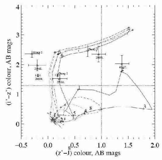
Figure 41: The combination of a $i-z$ and $z-J$ color cut permits the distinction of $z\simeq$5.7-6.5 star forming and $z\simeq$2 passive galaxies. Both may satisfy the $i-z>$1.5 dropout selector, but the former should lie blueward of the $z-J$=1.0 divider, whereas $z\simeq$2 are red in both colors. Crosses represent the location of candidates in the GOODS field and model tracks illlustrate the predicted colors for typical SEDs observed at the respective redshifts (Stanway et al 2005).

Unfortunately, the spectral properties of cool Galactic L dwarfs are dominated by prominent molecular bands rather than simply by their effective temperature. This means that they cannot be separated from $z\simeq$6 galaxies in a similar color-color diagram. Indeed, annoyingly, these dwarfs occupy precisely the location of the wanted $z\simeq$6 galaxies (Figure 42)! The only practical way to discriminate L dwarfs is either via spectroscopy or their unresolved nature in ACS images.

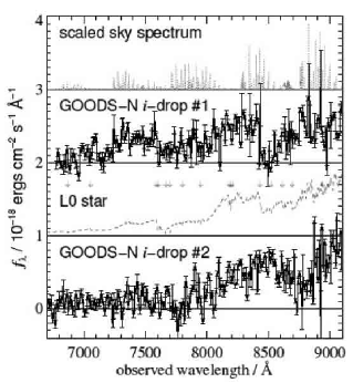
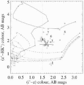
Figure 42: (Left) Keck spectroscopic verification of two contaminating L dwarfs lying within the GOODS $i-z$ dropout sample but pinpointed as likely to be stellar from ACS imaging data. The smoothed spectra represent high signal to noise brighter examples for comparison purposes. Strong molecular bands clearly mimic the Lyman dropout signature. (Right) Optical-infrared color diagram with the dropout color selector, $i_{AB}-z_{AB}>1.5$, shown as the vertical dotted line. Bright L dwarfs (lozenges) frustratingly occupy a similar region of color space as the $z\simeq$6 candidates (points with error bars) (Stanway et al 2004).

Stanway et al (2004) conducted the first comprehensive spectroscopic and ACS imaging survey of a GOODS $i$-drop sample limited at $z_{AB}<$25.6, finding that stellar contamination at the bright end of the luminosity function of a traditional ($i_{AB}-z_{AB}>$1.5) color cut could be as high as 30-40%. Unfortunately, even with substantial 6-8 hour integrations on the Keck telescope, redshift verification of the distant population was only possible in those dropout candidates with Ly$\alpha$ emission. Stanway et al (2005) subsequently analyzed the ACS imaging properties of a fainter subset arguing that stellar contamination decreases with increasing apparent magnitude.

Further progress has been possible via the use of the ACS grism on board HST (Malhotra et al 2005). As the OH background is eliminated in space, despite its low resolution, it is possible even in the fairly low signal/noise data achievable with the modest 2.5m aperture of HST to separate a Lyman break from a stellar molecular band. It is claimed that of 29 $z_{AB}<$27.5 candidates with (i-z)$>$0.9, only 6 are likely to be low redshift interlopers.

Regrettably, as a result of these difficulties, it has become routine to rely entirely on photometric and angular size information without questioning further the degree of contamination. This is likely one reason why there remain significant discrepancies between independent assessments of the abundance of $z\simeq$6 galaxies (Giavalisco et al 2004, Bouwens et al 2004, Bunker et al 2004). Although there are indications from the tests of Stanway et al (2004, 2005) and Malhotra et al (2005) that contamination is significant only at the bright end, the lack of a comprehensive understanding of stellar and foreground contamination remains a major uncertainty.

6.3 Cosmic Variance

The deepest data that has been searched for i-band dropouts includes the two GOODS fields (Dickinson et al 2004) and the Hubble Ultra Deep Field (UDF, Beckwith et al 2006). As these represent publicly-available fields they have been analyzed by many groups to various flux limits. The Bunker/Stanway team probed the GOODS fields to $z_{AB}$=25.6 (spectroscopically) and 27.0 (photometrically, and the UDF to $z_{AB}$=28.5. At these limits, it is instructive to consider the comoving cosmic volumes available in each field within the redshift range selected by the typical dropout criteria. For both GOODS-N/S fields, the total volume is $\simeq$5. 10⁵ Mpc³, whereas for the UDF it is only 2.6 10⁴ Mpc³. These contrast with 10⁶ Mpc³ for a single deep pointing taken with the SuPrime Camera on the Subaru 8m telescope.

Somerville et al (2004) present a formalism for estimating, for any population, the fractional uncertainty in the inferred number density from a survey of finite volume and angular extent. When the clustering signal is measurable, the cosmic variance can readily be calculated analytically. However, for frontier studies such as the i-dropouts, this is not the case. Here Somerville et al propose to estimate cosmic variance by appealing to the likely halo abundance for the given observed density using this to predict the clustering according to CDM models. In this way, the uncertainties in the inferred abundance of i-dropouts in the combined GOODS fields could be $\simeq$20-25% whereas that in the UDF could be as high as 40-50%.

It seems these estimates of cosmic variance can only be strict lower limits to the actual fluctuations since Somerville et al make the assumption that halos containing star forming sources are visible at all times. If, for example, there is intermittent activity with some duty cycle whose ”on/off” fraction is $f$, the cosmic variance will be underestimated by that factor $f$ (Stark et al, in prep).

6.4 Evolution in the UV Luminosity Density 3$<z<$10?

The complementary survey depths means that combined studies of GOODS and UDF have been very effective in probing the shape of the UV luminosity function (LF) at $z\simeq$6. Even so, there has been a surprising variation in the derived faint end slope $\alpha$. Bunker et al (2004) claim their data (54 i-dropouts) is consistent with the modestly-steep $\alpha$=-1.6 found in the $z\simeq$3 Lyman break samples (Steidel et 2003), whereas Yan & Windhorst (2004) extend the UDF counts to $z_{AB}$=30.0 and, based on 108 candidates, find $\alpha$=-1.9, a value close to a divergent function! Issues of sample completeness are central to understanding whether the LF is this steep.

In a comprehensive analysis based on all the extant deep data, Bouwens et al (2006) have attempted to summarize the decline in rest-frame UV luminosity density over 3$<z<$10 as a function of luminosity (Figure 43). They attribute the earlier discrepancies noted between Giavalisco et al (2004), Bunker et al (2004) and Bouwens et al (2004) to a mixture of cosmic variance and differences in contamination and photometric selection. Interestingly, they claim a luminosity-dependent trend in the sense that the bulk of the decline occurs in the abundance of luminous dropouts, which they attribute to hierarchical growth.

A similar trend is seen in ground-based data obtained with Subaru. Although HST offers superior photometry and resolution which is effective in eliminating stellar contamination, the prime focus imager on Subaru has a much larger field of view so that each deep exposure covers a field twice as large as both GOODS N+S. As they do not have access to ACS data over such wide fields, the Japanese astronomers have approached the question of stellar contamination in an imaginative way. Shioya et al (2005) used two intermediate band filters at 709nm and 826nm to estimate stellar contamination in both $z\simeq$5 and $z\simeq$6 broad-band dropout samples. By considering the slope of the continuum inbetween these two intermediate bands, in addition to a standard $i-z$ criterion, they claim an ability to separate L and T dwards. In a similar, but independent, study, Shimasaku et al (2005) split the $z$ band into two intermediate filters thereby measuring the rest-frame UV slope just redward of the Lyman discontinuity. These studies confirm both the redshift decline and, to a lesser extent, the luminosity-dependent trends seen in the HST data.

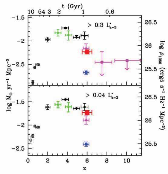
Figure 43: Evolution in the rest-frame UV (1350 Å ) luminosity density (right ordinate) and inferred star formation rate density ignoring extinction (left ordinate) for drop-out samples in two luminosity ranges from the compilation by Bouwens et al (2006). A marked decline is seen over $3<z<6$ in the contribution of luminous sources.

Although it seems there is a $5\times$ abundance decline in luminous UV emitting galaxies from $z\simeq$3 to 6, it’s worth noting again that the relevant counts refer to sources uncorrected for extinction. This is appropriate in evaluating the contribution of UV sources to the reionization process but not equivalent, necessarily, to a decline in the star formation rate density. Moreover, although the luminosity dependence seems similar in both ground and HST-based samples, it remains controversial (e.g. Beckwith et al 2006).

6.5 The Abundance of Star Forming Sources Necessary for Reionization

Have enough UV-emitting sources been found at $z\simeq$6-10 to account for cosmic reionization? Notwithstanding the observational uncertainties evident in Figure 43, this has not prevented many teams from addressing this important question. The main difficulty lies in understanding the physical properties of the sources in question. The plain fact is that we cannot predict, sufficiently accurately, the UV luminosity density that is sufficient for reionization!

Some years ago, Madau, Haardt & Rees (1999) estimated the star formation rate density based on simple parameterized assumptions concerning the stellar IMF and/or metallicity $Z$ essential for converting a 1350 Å luminosity into the integrated UV output, the fraction $f_{esc}$ of escaping UV photons, the clumpiness of the surrounding intergalactic hydrogen, $C=<\rho_{HI}^{2}>/<\rho_{HI}>^{2}$, and the temperature of the intergalactic medium $T_{IGM}$. In general terms, for reionization peaking at a redshift $z_{reion}$, the necessary density of sources goes as:

$$\rho\propto f_{esc}^{-1}\,C\,(1+z)^{3}\,(\Omega_{B}h^{2})^{2}Mpc^{-3}$$

For likely ranges in each of these parameters, Stiavelli et al (2004) tabulate the required source surface density which, generally speaking, lie above those observed at $z\simeq$6 (e.g. Bunker et al 2004).

It is certainly possible to reconcile the end of the reionization at $z\simeq$6 with this low density of sources (Figure 43) by appealing to cosmic variance, a low metallicity and/or top-heavy IMF (Stiavelli et al 2005) or a steep faint end slope of the luminosity function (Yan & Windhorst 2004) but none of these arguments is convincing without further proof. As we will see, the most logical way to proceed is to explore both the extent of earlier star formation from the mass assembled at $z\simeq$5-6 (Lecture 5) and to directly measure, if possible, the abundance of low luminosity sources at higher redshift.

6.6 The Spitzer Space Telescope Revolution: Stellar Masses at $z\simeq$6

One of the most remarkable aspects of our search for the most distant and early landmarks in cosmic history is that a modest cooled 85cm telescope, the Spitzer Space Telescope, can not only assist but provide crucial diagnostic data! The key instrument is the InfraRed Array Camera (IRAC) which offers four channels at 3.6, 4.5, 5.8 and 8$\mu$m corresponding to the rest-frame optical 0.5-1$\mu$m at redshifts $z\simeq$6-7. In the space of only a year, the subject has progressed from the determination of stellar masses for a few $z\simeq$5-7 sources to mass densities and direct constraints on the amount of early activity, as discussed in Lecture 5.

An early demonstration of the promise of IRAC in this area was provided by Eyles et al (2005) who detected two spectroscopically-confirmed $z\simeq$5.8 $i$-band dropouts at 3.6$\mu$m, demonstrating the presence of a strong Balmer break in their spectral energy distributions (Figure 44). In these sources, the optical detection of Ly$\alpha$ emission provides an estimate of the current ongoing star formation rate, whereas the flux longward of the Balmer break provides a measure of the past averaged activity. The combination gives a measure of the luminosity weighted age of the stellar population. In general terms, a Balmer break appears in stars whose age cannot, even in short burst of activity, be younger than 100 Myr. Eyles et al showed such systems could well be much older (250-650 Myr) depending on the assumed form of the past activity. As the Universe is only 1 Gyr old at $z\simeq$6, the IRAC detections gave the first indirect glimpse of significant earlier star formation - a glimpse that was elusive with direct searches at the time.

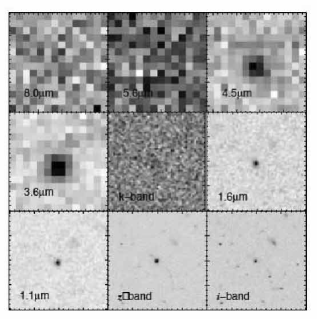
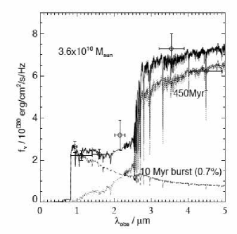
Figure 44: (Left) Detection of a spectroscopically-confirmed $i$-drop at $z$=5.83 from the analysis of Eyles et al (2005). (Right) Spectral energy distribution of the same source. Data points refer to IRAC at 3.6 and 4.5$\mu$m, VLT (K) and HST NICMOS (J,H) overplotted on a synthesised spectrum; note the prominent Balmer break. Synthesis models indicate the Balmer break takes 100 Myr to establish. However, the luminosity-weighted age could be significantly older depending on the assumed past star formation rate. In the example shown, a dominant 450 Myr component ($z_{F}\sim$10) is rejuvenated with a more recent secondary burst whose ongoing star formation rate is consistent with the Ly$\alpha$ flux observed in the source.

Independent confirmation of both the high stellar masses and prominent Balmer breaks was provided by the analysis of Yan et al (2005) who studied 3 $z\simeq$5.9 sources. Moreover, Yan et al also showed several objects had $(z-J)$ colors bluer than the predictions of the Bruzual-Charlot models for all reasonable model choices - a point first noted by Stanway et al (2004).

Eyles et al and Yan et al proposed the presence of established stellar populations in $z\simeq$6 $i$-drops and also to highlight the high stellar masses ($M\simeq 1-4\,10^{10}M_{\odot}$) they derived. At first sight, the presence of $z\simeq$6 sources as massive as the Milky Way seems a surprising result. Yan et al discuss the question in some detail and conclude the abundance of such massive objects is not inconsistent with hierarchical theory. In actuality it is hard to be sure because cosmic variance permits a huge range in the derived volume density and theory predicts the halo abundance (e.g. Barkana & Loeb 2000) rather than the stellar mass density. To convert one into the other requires a knowledge of the star formation efficiency and its associated duty-cycle.

One early UDF source detected by IRAC has been a particular source of puzzlement. Mobasher et al (2005) found a J-dropout candidate with a prominent detection in all 4 IRAC bandpasses. Its photometric redshift was claimed to be $z\simeq$6.5 on the basis of both a Balmer and a Lyman break. However, despite exhaustive efforts, its redshift has not been confirmed spectroscopically. The inferred stellar mass is 2-7 $10^{11}M_{\odot}$, almost an order of magnitude larger than the spectroscopically-confirmed sources studied by Eyles et al and Yan et al. If this source is truly at $z\simeq$6.5, finding such a massive galaxy whose star formation likely peaked before $z\simeq$9 is very surprising in the context of contemporary hierarchical models. Such sources should be extremely rare so finding one in the tiny area of the UDF is all the more puzzling. Dunlop et al (2006) have proposed the source must be foreground both on account of an ambiguity in the photometric redshift determination and the absence of similarly massive sources in a panoramic survey being conducted at UKIRT (McClure et al 2006).

This year, the first estimates of the stellar mass density at $z\simeq$5-6 have been derived (Yan et al 2006, Stark et al 2006a, Eyles et al 2006). Although the independenty-derived results are consistent, both with one another and with lower redshift estimates (Figure 45) the uncertainties are considerable as discussed briefly in the previous lecture. There are four major challenges to undertaking a census of the star formation at early times.

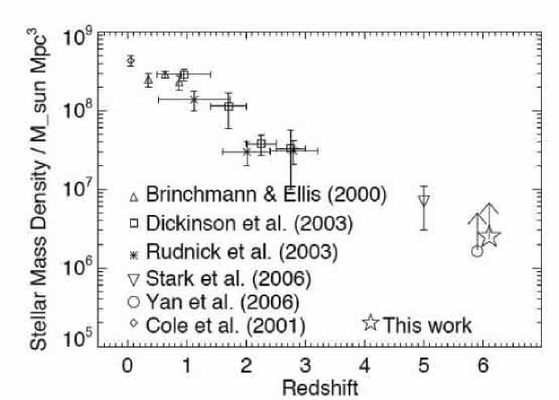
Figure 45: Evolution in the comoving stellar mass density from the compilation derived by Eyles et al (2006). The recent $z\simeq$5-6 estiimates constitute lower limits given the likelihood of quiescent sources missed by the drop-out selection technique. Results at $z\simeq$6 are offset slightly in redshift for clarity.

Foremost, the bulk of the faint sources only have photometric redshifts. Even a small amount of contamination from foreground sources would skew the derived stellar mass density upward. Increasing the spectroscopic coverage would be a big step forward in improving the estimates.

Secondly, IRAC suffers from image confusion given its lower angular resolution than HST (4 arcsec c.f. 0.1 arcsec). Accordingly, the IRAC fluxes cannot be reliably estimates for blended sources. Stark et al address this by measuring the masses only for those uncontaminated, isolated sources, scaling up their total by the fraction omitted. This assumes confused sources are no more or less likely to be a high redshift.

Thirdly, as only star forming sources are selected using the $v-$ and $i-$ dropout technique, if star formation is episodic, it is very likely that quiescent sources are present and thus the present mass densities represent lower limits. The missing fraction is anyone’s guess. As we saw at $z\simeq$2, the factor could be as high as $\times$2.

Finally, as with all stellar mass determinations, many assumptions are made about the nature of the stellar populations involved and their star formation histories. Until individual $z\simeq$5-6 sources can be studied in more detail, perhaps via the location of one or two strongly lensed examples, or via future more powerful facilities, this will regrettably remain the situation. At present, such density estimates are unlikely to be accurate to better than a factor of 2. Even so, they provide good evidence for significant earlier star formation (Stark et al 2006a, Lecture 5).

6.7 Lecture Summary

In this lecture we have discussed the great progress made in using $v,i,z$ and $J$ band Lyman dropouts to probe the abundance of star forming galaxies over 3$<z<$10. At redshifts $z\simeq$6 alone, Bouwens et al (2006) discuss the properties of a catalog of 506 sources to $z_{AB}$=29.5.

In practice, the good statistics are tempered by uncertain contamination from foreground cool stars and dusty or passively-evolving red $z\simeq$2 galaxies and the vagaries of cosmic variance in the small fields studied. It may be that we will not overcome these difficulties until we have larger ground-based telescopes.

Nonetheless, from the evidence at hand, it seems that the comoving UV luminosity density declines from $z\simeq$3 to 10, and that only by appealing to special circumstances can the low abundance of star forming galaxies at $z>$6 be reconciled with that necessary to reionize the Universe.

One obvious caveat is our poor knowledge of the contribution from lower luminosity systems. Some authors (Yan & Windhorst 2004, Bouwens et al 2006) have suggested a steepening of the luminosity function at higher redshift. Testing this assumption with lensed searches is the subject of our next lecture.

Finally, we have seen the successful emergence of the Spitzer Space Telescope as an important tool in confirming the need for star formation at $z>$6. Large numbers of $z\simeq$5-6 galaxies have now been detected by IRAC. The prominent Balmer breaks and high stellar masses argue for much earlier activity. Reconciling the present of mature galaxies at $z\simeq$6 with the absence of significant star formation beyond, is one of the most interesting challenges at the present time.

7 Lyman Alpha Emitters and Gravitational Lensing

7.1 Strong Gravitational Lensing - A Primer

Slowly during the twentieth century, gravitational lensing moved from a curiosity associated with the verification of General Relativity (Eddington 1919) to a practical tool of cosmologists and those studying distant galaxies. There are many excellent reviews of both the pedagogical aspects of lensing (Blandford & Narayan 1998, Mellier 2000, Refregier 2002) and a previous Saas-Fee contributor (Schneider 2006).

To explore the distant Universe, we are primarily concerned with strong lensing - where the lens has a projected mass density, above a critical value, $\Sigma_{crit}$, so that multiple images and high source magnifications are possible. For a simple thin lens

$$\Sigma_{crit}=\frac{c^{2}\,D_{OS}}{4\,\pi\,G\,D_{OL}\,D_{LS}}$$

where $D$ represents the angular diameter distance and the subscripts $O,L,S$ refer to the observer, source and lens, respectively. Rather conveniently, for a lens at $z\simeq$0.5 and a source at $z>$2, the critical projected density is about 1 g cm^-2 - a value readily exceeded by most massive clusters. The merits of exploring the distant Universe by imaging through clusters was sketched in a remarkably prophetic article by Zwicky (1937).

In lensing theory it is convenient to introduce a source plane, the true sky, and an image plane, the detector at our telescope, where the multiple images are seen. The relationship between the two is then a mapping transformation which depends on the relative distances (above). Crucially, what the observer sees depends on the degree of alignment between the source and lens as illustrated in Figure 46.

An elliptical lens with $\Sigma>\Sigma_{crit}$ for a given source and lens distance produces a pair of critical lines in the image plane where the multiple images lie. These lines map to caustics in the source plane. The outer critical line is equivalent to the Einstein radius $\theta_{E}$

$$\theta_{E}=\sqrt{\frac{4\,G\,M\,D_{OS}}{c^{2}\,D_{OL}\,D_{LS}}}$$

and, for a given source and lens, is governed by the enclosed mass $M$. The location of the inner critical line depends on the gradient of the gravitational potential (Sand et al 2005).

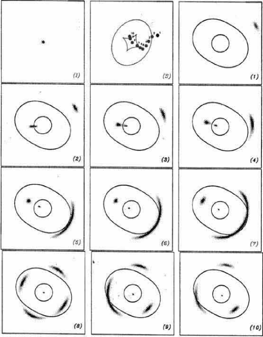
Figure 46: Configurations in the image plane for an elliptical lens as a function of the degree of alignment between the source and lens (second panel). Lines in the source plane refer to ‘caustics’ which map to ‘critical lines’ in the image plane (see text for details). (Courtesy of Jean-Paul Kneib)

The critical lines are important because they represent areas of sky where very high magnifications can be encountered - as high as $\times$30! For $\simeq$20 well-studied clusters the location of these lines can be precisely determined for a given source redshift. Accordingly, it is practical to survey just those areas to secure a glimpse of otherwise inaccessibly faint sources boosted into view. The drawback is that, as in an optical lens, the sky area is similarly magnified, so the surface density of faint sources must be very large to yield any results. Regions where the magnification exceed $\times$10 are typically only 0.1-0.3 arcmin² per cluster in extent in the image plane and inconveniently shaped for most instruments (Figure 47). The sampled area in the source plane is then ten times smaller so to see even one magnified source/cluster requires a surface density of distant sources of $\sim$50 arcmin^-2.

Two other applications are particularly useful in faint galaxy studies. Firstly, strongly magnified systems at $z\simeq$2-3 can provide remarkable insight into an already studied population by providing an apparently bright galaxy which is brought within reach of superior instrumentation. cB58, a Lyman break galaxy at $z$=2.72 boosted by $\times$30 to $V$=20.6 (Yee et al 1996, Seitz et al 1998) was the first distant galaxy to be studied with an echellette spectrograph (Pettini et al 2002), yielding chemical abundances and outflow dynamics of unprecedented precision.

More generally, a cluster can magnify a larger area of $\simeq$2-4 arcmin² by a modest factor, say $\times$3-5. This has been effective in probing sub-mm source counts to the faintest possible limits (Smail et al 1997) and the method shows promise for similar extensions with the IRAC camera onboard Spitzer.

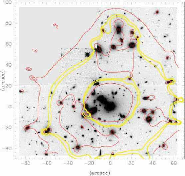
Figure 47: Hubble Space Telescope image of the rich cluster Abell 1689 with the critical lines for a source at $z\simeq$5 overlaid in yellow. The narrow regions inbetween the pairs of yellow lines refer to regions where the magnification exceeds $\times$10.

7.2 Creating a Cluster Mass Model

In the applications discussed above, in order to analyze the results, the inferred magnification clearly has to be determined. This will vary as a function of position in the cluster image and the relative distances of source and lens. The magnification follows from the construction of a mass model for the cluster.

The precepts for this method are discussed in the detailed analysis of the remarkable image of Abell 2218 taken with the WFPC-2 camera onboard HST in 1995 (Kneib et al 1996). An earlier image of AC 114 showed the important role HST would play in the recognition of multiple images (Smail et al 1995). Prior to HST, multiple images could only be located by searching for systems with similar colors, using the fact that lensing is an achromatic phenomenon. HST revealed that morphology is a valuable additional identifier; the improved resolution also reveals the local shear (see Figure 48).

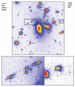
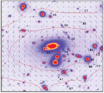
Figure 48: Hubble Space Telescope study of the rich cluster AC114 (Smail et al 2005) (Top) Morphological recognition of a triply-imaged source. The lower inset panels zoom in on each of 3 images of the same source. (Bottom) Construction of mass contours (red lines) and associated shear (red vectors) from the geometrical arrangement of further multiple images labelled A1-3, B1-4, C1-3, Q1-3.

Today, various approaches are possible for constructing precise mass models for lensing clusters (Kneib et al 1996, Jullo et al 2006, Broadhurst et al 2005). These are generally based on utilizing the geometrical positions of sets of multiply-imaged systems whose redshift is known or assumed. This then maps the form and diameter of the critical line for a given $z$. Spectroscopic redshifts are particularly advantageous, as are pairs that straddle the critical line whose location can then be very precisely pinpointed. A particular mass model can be validated by ‘inverting’ the technique and predicting the redshifts of other pairs prior to subsequent spectroscopy (Ebbels et al 1999).

The main debate among cognescenti in this area lies in the extent to which one should adopt a parametric approach to fitting the mass distribution, particularly in relation to the incorporation of mass clumps associated with individual cluster galaxy halos (Broadhurst et al 2005). Stark et al (2006b) discuss the likely uncertainties in the mass modeling process arising from the various techniques.

7.3 Lensing in Action: Some High $z$ Examples

Before turning to Lyman $\alpha$ emitters (lensed and unlensed), we will briefly discuss what has been learned from strongly-lensed dropouts.

Figure 49 shows a lensed pair in the cluster Abell 2218 ($z$=0.18) as detected by NICMOS onboard HST and the two shortest wavelength channels of IRAC (Kneib et al 2004, Egami et al 2005). Although no spectroscopic redshift is yet available for this source, three images have been located by HST and their arrangement around the well-constrained $z$=6 critical line suggests a source beyond $z\simeq$6 (Kneib et al 2004).

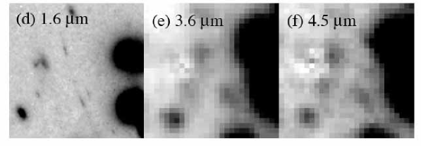
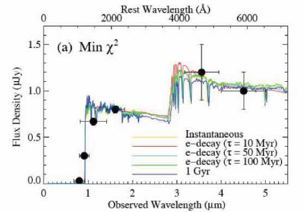
Figure 49: (Top) Lensed pair of a $z$=6.8 source as seen by NICMOS and IRAC in the rich cluster Abell 2218 (Egami et al 2005). The pair straddles the critical line at $z\simeq$6 and a fainter third image at a location predicted by the lensing model has been successfully recovered in the HST data (Kneib et al 2004). (Bottom) Spectral energy distribution of the source revealing a significant Balmer break and improved estimates of the star formation rate, stellar mass and luminosity weighted age.

As with the unlensed $i$-band drop out studies by Eyles et al (2005) and Yan et al (2005), the prominent IRAC detections (Egami et al 2005) permit an improved photometric redshift and important constraints on the stellar mass and age. A redshift of $z$=6.8$\pm$0.1 is derived, independently of the geometric constraints used by Kneib et al. The stellar mass is $\simeq$5-10 10${}^{8}M_{\odot}$ and the current star formation rate is $\simeq$2.6 M_⊙ yr^-1. The luminosity-weighted age corresponds to anything from 40-450 Myr for a normal IMF depending on the star formation history. Interestingly, the derived age for such a prominent Balmer break generally exceeds the e-folding timescale of the star formation history (Fig. 49) indicating the source would have been more luminous at redshifts $7<z<$12 (unless obscured).

Given the small search area used to locate this object, such low mass sources may be very common. Accordingly, several groups are now surveying more lensing clusters for further examples of $z$ band dropouts and even $J$-band dropouts (corresponding to $z\simeq$8-10) . Richard et al are surveying 6 clusters with NICMOS and IRAC with deep ground-based $K$ band imaging from Subaru and Keck. In these situations, one has to distinguish between magnifications of $\times$5 or so expected across the 2-3 arcmin fields of NICMOS and IRAC, and the much larger magnifications possible close to the critical lines. Contamination from foreground sources should be similar to what is seen in the GOODS surveys discussed in Lecture 6. The discovery of image pairs in the highly-magnified regions would be a significant step forward since spectroscopic confirmation of any sources at the limits being probed ($H_{AB}\simeq$26.5-27.0) will be exceedingly difficult.

7.4 Lyman alpha Surveys

The origin and characteristic properties of the Lyman $\alpha$ emission line has been discussed by my colleagues in their lectures (see also Miralda-Escude 1998, Haiman 2002, Barkana & Loeb 2004 and Santos 2004). The $n$=2 to 1 transition corresponding to an energy difference of 10.2 eV and rest-wavelength of $\lambda$1216 Å  typically arises from ionizing photons absorbed by nearby hydrogen gas. The line has a number of interesting features which make it particularly well-suited for locating early star forming galaxies as well as for characterizing the nature of the IGM.

In searching for distant galaxies, emission lines offer far more contrast against the background sky than the faint stellar continuum of a drop-out. A line gives a convincing spectroscopic redshift (assuming it is correctly identified) and models suggest that as much as 7% of the bolometric output of young star-forming region might emerge in this line. For a normal IMF and no dust, a source with a star formation rate (SFR) of 1 $M_{\odot}$ yr^-1 yields an emission line luminosity of 1.5 10⁴² ergs sec^-1.

Narrow band imaging techniques (see below) can reach fluxes of $<$ 10^-17 cgs in comoving survey volumes of $\simeq$10⁵ Mpc³, corresponding to a SFR $\simeq$3 $M_{\odot}$ yr^-1 at $z\simeq$6. Spectroscopic techniques can probe fainter due to the improved contrast. This is particularly so along the critical lines where the additional boost of gravitational lensing enables fluxes as faint as 3. 10^-19 cgs to be reached (corresponding to SFR $\simeq$0.1 $M_{\odot}$ yr^-1). However, in this case the survey volumes are much smaller ($\simeq$50 Mpc³). In this sense, the two techniques (discussed below) are usefully complementary.

Having a large dynamic range in surveys for Ly$\alpha$ emission is important not just to probe the luminosity function of star-forming galaxies but also because it can be used to characterize the IGM. As a resonant transition, foreground hydrogen gas clouds can scatter away Ly$\alpha$ photons in both direction and frequency. In a partially ionized IGM, scattering is maximum at $\lambda$1216 Å in the rest-frame of the foreground cloud, thus affecting the blue wing of the observed line. However, in a fully neutral IGM, scattering far from resonance can occur leading to damping over the entire observed line. Figure 50 illustrates how, in a hypothetical situation where the IGM becomes substantially neutral during 6$<z<$7, surveys reaching the narrow-band flux limit would still find emitters at $z$=7. Their intense emission would only be partially damped by even a neutral medium. However, lines with fluxes at the spectroscopic lensing limit would not survive. Accordingly, one possible signature of reionization would be a significant change in the shape of the Ly$\alpha$ luminosity function at the faint end (Furlanetto et al 2005).

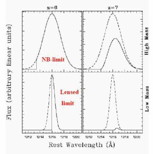
Figure 50: The Lyman $\alpha$ damping wing is absorbed by neutral hydrogen and thus can act as a valuable tracer of the nature of the IGM. The simulation demonstrates the effect of HI damping on emission lines in high mass and low mass systems (characteristic of sources detected in typical narrow band and lensed spectroscopic surveys respectively) assuming reionization ends inbetween $z$=6 and 7. The dramatic change in visibility of the weaker systems suggests their study with redshift may offer a sensitive probe of reionization. Courtesy: Mike Santos.

7.5 Results from Narrow Band Ly$\alpha$ Surveys

The most impressive results to date have come from various narrow-band filters placed within the SuPrime camera at the prime focus of the Subaru 8m telescope (Kodaira et al 2003, Hu et al 2004, Ouchi et al 2005, Taniguchi et al 2005, Shimasaku et al 2006, Kashikawa et al 2006, Iye et al 2006). Important conclusions have also been deduced from an independent 4m campaign (Malhotra & Rhoads 2004).

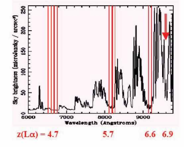
Figure 51: Night sky spectrum and the deployment of narrow band filters in ‘quiet’ regions corresponding to redshifted Lyman $\alpha$ emission as indicated below. The final optical window, corresponding to $z\simeq$6.9, was successfully exploited by Iye et al (2006) to find two sources close to $z\simeq$7.

Narrow band filters are typically manufactured at wavelengths where the night sky spectrum is quiescent, thus maximizing the contrast. These locations correspond to redshifts of $z$=4.7, 5.7, 6.6 and 6.9 (Fig. 52). A recent triumph was the successful recovery of two candidates at $z\simeq$6.96 by Iye et al (2006). Candidates are selected by comparing their narrow band fluxes with that in a broader band encompassing the narrow band wavelength range. The contrast can then be used as an indicator of line emission (Fig. 53). Spectroscopic follow-up is still desirable as the line could arise in a foregound galaxy with [O II] 3727 Å or [O III] 5007 Å emission. The former line is a doublet and the latter is part of a pair with a fixed line ratio, separated in the rest-frame by only 60 Å or so, so these contaminants are readily identified. Furthermore, Ly$\alpha$ is often revealed by its asymmetric profile (c.f. Fig. 51).

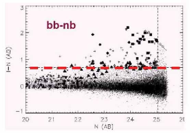
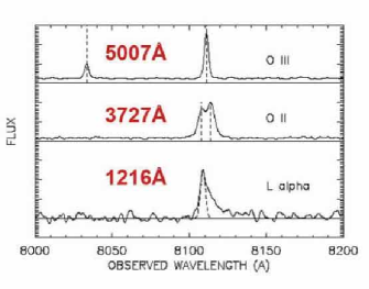
Figure 52: The two-step process for locating high redshift Lyman $\alpha$ emitters (Hu et al 2004). (Left) Comparison of broad and narrow band magnitudes; sources with an unusual difference in the sense of being brighter in the narrow band filter represent promising candidates. (Right) Spectroscopic follow-up reveals typically three possibilities - [O III] or [O II] at lower redshift, or Ly$\alpha$ often characterized by its asymmetric line profile.

Spectroscopic follow-up is obviously time-intensive for a large sample of candidates, hundreds of which can now be found with panoramic imagers such as SuPrimeCam. Therefore it is worth investigating additional ways of eliminating foreground sources. Tanuguchi et al (2005) combine the narrow band criteria adopted in Fig. 53 with a broad-band $i-z$ drop-out signature. Spectroscopic follow-up of candidates located via this double color cut revealed a 50-70% success rate for locating high $z$ emitters. The drawback is that the sources so found cannot easily be compared in number with other, more traditional, methods. Nagao et al (2005) used a narrow - broad band color criterion in the opposite sense, locating sources with a narrow band depression (rather than excess). Such rare sources are confirmed to be sources with extremely intense emission elsewhere in the broad-band filter. Such sources, with Lyman $\alpha$ equivalent widths in excess of several hundred Å are interesting because they may challenge what can be produced from normal stellar populations.

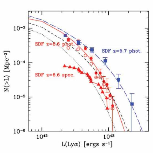
Figure 53: Comparison of the Lyman $\alpha$ luminosity functions at $z$=5.7 and 6.5 from the surveys of Kashikawa et al (2006) and Shimasaku et al (2006); both spectroscopically-confirmed and photometric candidates are plotted. The decline in luminous emitters is qualitatively similar to trends seen over 3$<z<$6 in luminous continuum drop-outs.

Malhotra & Rhoads (2004) were the first to consider the absence of evolution in the Ly$\alpha$ LF as a constraint on the neutral fraction. Although they found no convincing change in the LF between $z$=5.7 and 6.5, the statistical uncertainties in both LFs were considerable. Specifically, below luminosities of $L_{Ly\alpha}\simeq$10^42.5 ergs sec^-1 no detections were then available. Hu et al (2005) have also appealed to the absence of any significant change in the mean Ly$\alpha$ profile. Malhotra & Rhoads deduced the neutral fraction must be $x_{HI}<$0.3 at $z\simeq$6 supporting early reionization. However, Furlanetto et al (2005) reanalyzed this constraint and indicated that strong emitters could persist even when $x_{HI}\simeq$0.5 (c.f. Fig. 51).

Kashikawa et al (2006) and Shimasaku et al (2006) have determined statistically greatly improved Lyman $\alpha$ luminosity functions and discuss both spectroscopic confirmed and photometrically-selected emitters (Fig. 53). No decline is apparent in the abundance of low luminosity emitters as expected in an IGM with high $x_{HI}$; indeed the most significant change is a decline with redshift in the abundance of the most luminous systems. Although the change seems surprisingly rapid given the time interval is only 150 Myr, this is consistent with growth in the halo mass function (Dijsktra et al 2006).

7.6 Results from Lensed Ly$\alpha$ Surveys

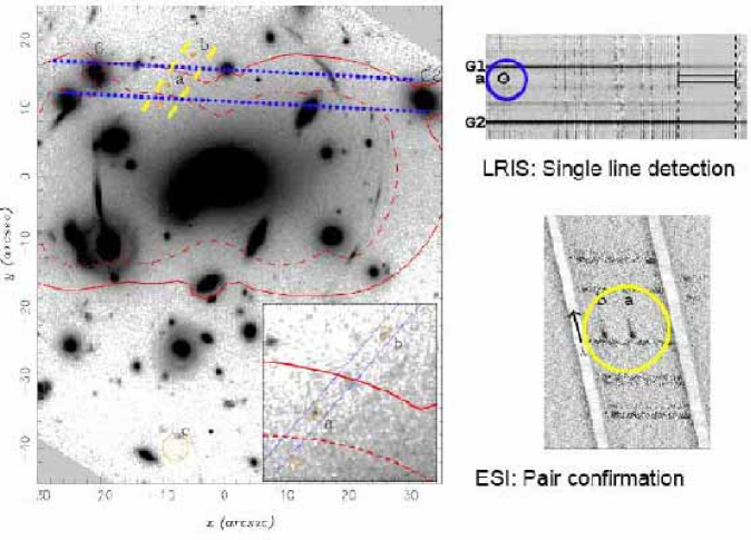
Figure 54: Critical line mapping in Abell 2218: how it works (Ellis et al 2001). The red curves show the location of the lines of very high magnification for a source at a redshift $z$=1 (dashed) and $z$=6 (solid). Blue lines show the region scanned at low resolution with a long-slit spectrograph. The upper right panel shows the detection of an isolated line astrometrically associated with (a) in the HST image for which a counter image (b) is predicted and recovered (see also inset to main panel). A higher dispersion spectrum aligned between the pair (yellow lines) reveal strong emission with an asymmetric profile in both (lower right panel).

The principal gain of narrow band imaging over other techniques in locating high redshift Lyman $\alpha$ emitters lies in the ability to exploit panoramic cameras with fields of view as large as 30-60 arcmin. Since cosmic lenses only magnify fields of a few arcmin or less, lensing searches are only of practical utility when used in spectroscopic mode. As discussed above, the gain in sensitivity can be factors of $\times$30 or more, and given the small volumes explored, they are primarily useful in testing the faint end of the Ly$\alpha$ luminosity function at various redshifts. A number of workers (e.g. Barkana & Loeb 2004) have emphasized the likelihood that the bulk of the reionizing photons arise from an abundant population of intrinsically-faint sources, and lensed searches provide the only practical route to observationally testing this hypothesis.

A practical demonstration of a blind search for lensed Ly$\alpha$ emitters is summarized in Figure 54. A long slit is oriented along a straight portion of the critical line (whose location depends on the source redshift). The survey comprises several exposures taken in different positions offset perpendicular to the critical line. Candidate emission lines are astrometrically located on a deep HST image and, if a counter-image consistent with the mass model can be located, a separate exposure is undertaken to capture both (as was the case in the source located by Ellis et al 2001). Unfortunately, continuum emission is rarely seen from a faint emitter and the location of a corresponding second image is often too uncertain to warrant a separate search. In this case contamination from foreground sources has to be inferred from the absence of corresponding lines at other wavelengths (Santos et al 2004, Stark et al 2006b).

Using this technique with an optical spectrograph sensitive to Ly$\alpha$ from 2.2$<z<$6.7, Santos et al (2004) conducted a survey of 9 lensing clusters and found 11 emitters probing luminosities as faint as $L_{Ly\alpha}\simeq 10^{40}$ cgs, significantly fainter than even the more recent Subaru narrow band imaging searches (Shimasaku et al 2006). The resulting luminosity function is flatter at the faint end than implied for the halo mass function and is consistent with suppression of star formation in the lowest mass halos.

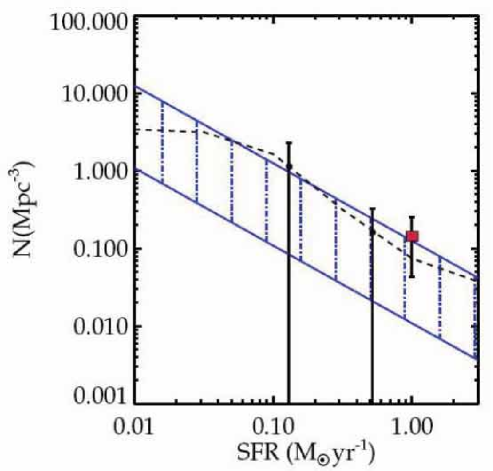
Figure 55: The volume density of sources of various star formation rates at $z\simeq$8-10 required for cosmic reionization for a range of assumed parameters (blue hatched region) compared to the inferred density of lensed emitters from the survey of Stark et al (2006b). The open red symbol corresponds to the case if all detected emitters are at $z\simeq$10, the black symbols correspond to the situation if the two most promising candidates are at $z\simeq$10, and the dashed line corresponds to the 5$\sigma$ upper limit if none of the candidates is at $z\simeq$10.

Stark et al (2006b) have extended this technique to higher redshift using an infrared spectrograph operating in the $J$ band, where lensed Ly$\alpha$ emitters in the range 8.5$<z<$10.2 would be found. This is a much more demanding experiment than that conducted in the optical because of the brighter and more variable sky brightness, the smaller slit length necessitating very precise positioning to maximize the magnifications and, obviously, the fainter sources given the increased redshift. Nonetheless, a 5$\sigma$ sensitivity limit fainter than 10^-17 cgs corresponding to intrinsic (unlensed) star formation rates of 0.1 $M_{\odot}$ yr^-1 is achieved with the 10m Keck II telescope in exposure times of 1.5 hours per slit position.

After surveying 10 clusters with several slit positions per cluster, 6 candidate emission lines have been found and, via additional spectroscopy, it seems most cannot be explained as foreground sources. Stark et al estimate the survey volume taking into account both the spatially-dependent magnification (from the cluster mass models) and the redshift-dependent survey sensitivity (governed by the night sky spectrum within the spectral band).

Madau et al (1999) and Stiavelli et al (2004) have introduced simple prescriptions for estimating the abundance of star forming sources necessary for cosmic reionizations. While these prescriptions are certainly simple-minded, given the coarse datasets at hand, they provide an illustration of the implications.

Generally, the abundance of sources of a given star formation rate SFR necessary for cosmic reionization over a time interval $\Delta\,t$ is

$$n\propto\frac{B\,n_{H}}{f_{c}\,SFR\,\Delta\,t}$$

where $B$ is the number of ionizing photons required to keep a single hydrogen atom ionized, $n_{H}$ is the comoving number density of hydrogen at the redshift of interest and $f_{c}$ is the escape fraction of ionizing photons. Figure 56 shows the upshot of the Stark et al (2006b) survey for various assumptions. The detection of even a few convincing sources with SFR $\simeq$0.1-1 $M_{\odot}$ yr^-1 in such small cosmic volumes would imply a significant contribution from feeble emitters at $z\simeq$10. Although speculative at this stage given both the uncertain nature of the lensed emitters and the calculation above, it nonetheless provides a strong incentive for continued searches.

7.7 Lecture Summary

In this lecture we have shown how Lyman $\alpha$ emission offers more than simply a way to locate distant galaxies. The distribution of line profiles, equivalent widths and its luminosity function can act as a sensitive gauge of the neutral fraction because of the effects of scattering by hydrogen clouds. Surveys have been undertaken using optical cameras and narrow band filters to redshifts $z\simeq$7.

However, despite great progress in the narrow-band surveys, as with the earlier $i$-band drop outs, there is some dispute as to the evolutionary trends being found. Surprisingly strong evolution is seen in luminous emitters over a very short period of cosmic time corresponding to 5.7$<z<$6.5. And, to date there is no convincing evidence that line profiles are evolving or that the equivalent width distribution of emitters is skewed beyond what can be accounted for by normal young stellar populations. One suspects we will have to push these techniques to higher redshift which will be hard given the Ly$\alpha$ line moves into the infrared where no such panoramic instruments are yet available.

We have also given a brief tutorial on strong gravitational lensing. In about 20 or so clusters, spectroscopic redshifts for sets of multiple images has enabled quite precise mass models to be determined which, in turn, enable accurate magnification maps to be derived. Remarkably faint sources can be found by searching along the so-called critical lines where the magnification is high. The techniques has revealed a few intrinsically faint sources and, possibly, the first glimpse of a high abundance of faint star forming sources at $z\simeq$10 has been secured.

8 Cosmic Infrared Background

8.1 Motivation

In this lecture we examine the role of cosmic backgrounds. First we make an important distinction. We are primarily concerned with extragalactic backgrounds composed of unresolved faint sources rather than the fairly isotropic microwave radiation that comes from the recombination of hydrogen. Such unresolved source background have played a key role in astrophysics.

The pattern of discovery outside the optical and near-infrared spectral windows often goes like the following; the background is first discovered by sensitive detectors which do not have the angular resolution to see if there is any fine structure from faint sources. There is then some puzzlement as to its origin: for example, does it arise from an unforeseen population of sources beyond those already counted? In this manner, the X-ray background was identified as arising from active galactic nuclei and the sub-mm background from dusty star-forming galaxies. In each case we are concerned with separating the counts of resolved sources to some detectability limit with the measured value of the integrated background. Key issues relate to the contribution of resolved sources and the removal of spurious (non-extragalactic) foreground signals. Excellent reviews of the subject have been provided by Leinert et al (1998), Hauser & Dwek (2001) and Kashlinksy (2005).

In our case, we are interested in extending source counts of star forming galaxies beyond $z\simeq$6 and so the question of a near-infrared extragalactic background signal is of greatest relevance. The instruments concerned include cameras on Hubble Space Telescope and Spitzer SpaceTelescope, but other space missions such as COBE and the Infrared Telescope in Space have provided important results.

8.2 Methodogy

To understand the distinction between the resolved and unresolved components of the background, it is helpful to derive some fundamental relations for galaxy counts.

In the magnitude system, the differential count slope $\gamma$ with increasing magnitude is

$$\gamma=\frac{d\,log\,N(m)}{dm}$$

where $N(m)$ is the differential number of galaxies per unit sky area (e.g. deg^-2) in some counting bin $dm$.

Now the contribution to the surface brightness of the extragalactic night sky from sources as a given magnitude $m$ is:

$$i_{\nu}(m)=10^{-0.4(m+const)}\,N(m)$$

where the 0.4 factor arises from the relationship between flux and magnitude.

And the integrated surface brightness (the extragalactic background light, EBL) is obtained by extending this integral to infinitely faint limits, viz:

$$I_{\nu}=\int_{-\infty}^{\infty}i_{\nu}(m)\,dm$$

The bolometric equivalent of the EBL is then $\int I_{\nu}\,d\nu$. The EBL is often alternatively expressed as EBL = $\int\nu\,I_{\nu}\d{\,}d\nu$.

Surface brightness is usually expressed in nW m^-2 steradian^-1 although very early articles refer to some derivative of magnitudes deg^-2. As infrared fluxes are often expressed in Janskies (1 Jansky = 10^-26 W m^-2 Hz^-1, a useful conversion is 1 nw m^-2 ster^-1 = 3000/$\lambda(\mu$ m) MJy ster^-1.

Examination of the above relation shows that if $\gamma>$0.4, the surface brightness contribution from fainter sources outshines that of brighter ones and so the EBL will diverge. By deduction, therefore, the maximum contribution of resolved sources to the background will be where $\gamma\simeq$0.4. If the slope of the counts turns down below 0.4 at some point, it may seem pointless to speculate that there is much information from fainter unresolved sources. In the case of searching for cosmic reionization however, where the first sources may be a distinct population, continuity in the source counts may not be expected. For this reason, the interesting quantity is the difference between a measured EBL and the integrated contribution from the faintest resolved sources.

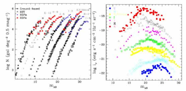
Figure 56: (Left) Differential galaxy counts as a function of wavelength from the compilation of Madau & Pozzetti (2000). Note the absolute numbers have been arbitrarily scaled for convenience. (Right) Magnitude-dependent contribution of the counts to the surface brightness $i_{\nu}$ of the extragalactic night sky. Depending on the waveband, the peak contribution occurs at $m_{AB}\simeq$20-25.

Madau & Pozzetti (2000) present a careful analysis of the deep optical and near-infrared counts at various wavelengths, mostly from Hubble Space Telescope data prior to the Ultra Deep Field (Figure 56). Extrapolation of the counts enables the contribution to the integrated light from known populations to be evaluated as a function of wavelength. The total EBL from this analysis is 55 nW m^-2 sr^-1 of which the dominant component lies longward of 1$\mu$m. However, it must be remembered that galaxies are extended objects and so it is possible that significant light is lost in the outermost regions of each. As surface brightness is relativistically dimmed by the cosmic expansion, $\propto(1+z)^{4}$, the contribution from distant sources could be seriously underestimated (Lanzetta et al 2002).

In a similar fashion to the check we made that the integrated star formation history produces the present stellar mass density (Lecture 4), so it is possible to verify that the bolometric output from stellar evolution should be consistent with the present mass density of stars.

The bolometric radiation density $\rho_{bol}(t)$ is

$$\rho_{bol}(t)=\int_{0}^{t}L(\tau)\dot{\rho_{s}}(t-\tau)d\,\tau$$

where $\dot{\rho_{s}}$ is the star formation rate per comoving volume.

The integrated EBL is then

$$I_{EBL}=\frac{c}{4\pi}\,\int_{t_{F}}^{t_{H}}\frac{\rho_{bol}(t)}{1+z}\,dt$$

The check is a little bit trickier because a typical star formation history has to be assumed and presumably there is a large variety for different kinds of sources observed at various redshifts. The issue is discussed in detail by Madau & Pozzetti.

8.3 Recent Background Measurements

The goal for making extragalactic background light (EBL) measures is thus to determine the extent to which the measured value (or limit) exceeds that predicted from extrapolation of the galaxy counts. This might then provide some evidence for a new distant population such as the sources responsible for cosmic reionization.

Figure 57: Summary of recent measures of the extragalactic background light from the compilation of Dole et al (2006). The cross-hatched region represents the region of claimed excess between the various background meaasures (labelled points) and the lower limits to the integrated counts (shown as upward arrows in the critical optical-near IR region). Interesting excesses are found in the 0.3 to 5 $\mu$m region.

Various claims of an excess have been made in the 0.3 to 10$\mu$m wavelength region (Figure 57). Outside of this window the background appears to be entirely produced by known sources. Such EBL measurements are extremely difficult to make for several reasons. An accurate absolute calibration is essential since the interesting signal is a ‘DC difference’ in surface brightness. The removal of spurious foregrounds is likewise troublesome: at some wavelengths, the foreground signal greatly exceeds the sought-after effect.

In the optical window, careful experiments have been undertaken by Mattila (1976), Dube et al (1979) and most recently Bernstein et al (2002). The most vexing foreground signals at optical wavelengths arise from airglow (emission in the upper atmosphere which has a time-dependent structure on fine angular scales), zodiacal light (scattering of sunlight by interplanetary dust which varies with the motion of the Earth along the ecliptic plane) and diffuse Galactic light or ‘cirrus’ (gas clouds illuminated by starlight). The wavelength dependence of these foregrounds (including the microwave background itself which is considered a ‘contaminant’ in this respect!) is summarized in Figure 58. For the critical near-infrared region where redshifted light from early sources might be detected, airglow and zodiacal light are the dominant contaminants.

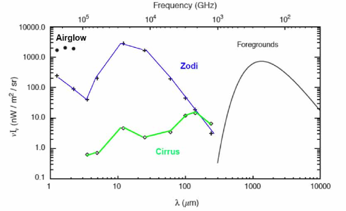
Figure 58: Wavelength dependence of the dominant foreground signals from the compilation by Kashlinsky (2005). Airglow and zodiacal light dominate at the wavelengths of interest for stellar radiation from highly redshift sources.

Experiments have differed in the way these foregrounds might be removed. The use of a space observatory avoids airglow and observations at different Galactic latitudes can be used to monitor or minimize the effect of cirrus. Zodiacal light, the dominant foreground for all mid-infrared studies and all space-based near-infrared studies, is the most troublesome.

To first order, the zodiacal light can be predicted depending on the geometrical configuration of the ecliptical plane, the earth, sun and target field. Although seasonal variations can be tracked and the spectrum of the zodiacal light is solar, imponderables enter such as the nature and distribution of the interplanetary dust and its scattering properties.

The positive EBL excess measures at optical to near-infrared wavelengths have remained controversial. This is because all such experiments search for a ‘DC signal’ - a small absolute difference between two signals within which foregrounds have to be painstakingly removed. A brief study of the Bernstein et al (2002) experiment will make the difficulties clear.

Bernstein et al (2002) claim a significant optical excess at 300, 550 and 800nm from fields observed with Hubble’s WFPC-2 and FOS. Airglow is elminated since HST is above 90km and sources were removed in each HST image to $V_{AB}$=23.0. The zodiacal light spectrum was measured simultaneously with a ground-based optical telescope and iteratively subtracted from the HST data.

At 550nm, the total WFPC-2 background measured after removing all sources was 105.7 $\pm$ 0.3 units (1 unit = 10^-9 cgs ster^-1 Å ^-1). The measured zodi background was 102.2 $\pm$0.6 units. Galactic cirrus and faint galaxies beyond $V_{AB}$=23.0 were estimated as 0.8 and 0.5 units respectively. The claimed excess signal at this wavelength is 2.7$\pm$1.4 units. Not only is this only a 2 $\sigma$ detection but it would only require a 2% error in the estimated Zodiacal light signal to be spurious.

Studies of the infrared background advanced significantly with the launch of the COBE satellite which carried DIRBE - a 10 channel photometer operating in the 1-240 $\mu$m range with 0.7 degree resolution chopping at 32Hz onto an internal zero flux surface, and FIRAS - an absolute spectrometer with 7 degree resolution operating in the 100 $\mu$m to 5mm range.

DIRBE measured the integrated background at 140 and 240$\mu$m using an elaborate time-dependent model of the Zodiacal light (Kelsall et al 1998, Hauser et al 1998). Schlegel et al (1998) combined these data with higher resolution IRAS 100$\mu$m maps to improve removal of Galactic cirrus and to measure the temperature of the dust emission. Finkbeiner et al (2000) extended the model of Zodiacal light to provide the first detection at 60 and 100$\mu$m and Wright & Reese (2000) used 2MASS observations to improve Galactic source removal claiming a detection at 2.2$\mu$m.

Dole et al (2006) have undertaken a very elegant analysis of 19000 Spitzer MIPS images. By centering the images on deep 24$\mu$m sources, they can evaluate the statistical contribution of otherwise inaccessibly faint 70 and 160 $\mu$m sources.

Matsumoto et al (2005) has extended these detections to shorter wavelengths using a spectrometer onboard the Infrared Telescope in Space (IRTS). This signal has the tantalising signature of a distant star-forming stellar population - a steeply-rising continuum down to 1$\mu$m and a discontinuity when extended to include optical data (Figure 57). Mattila (2006) has argued this signal represents an artefact arising from incorrect foreground removal. He has likewise criticised the Bernstein et al (2002) optical detections (Mattila 2003).

Supposing the DIRBE/2MASS/IRTS detections to be real, what would this imply? Assuming the J-band background ($>$2.5 nW m^-2 ster^-1) arises from $z\simeq$9 Ly$\alpha$ emission, Madau & Silk (2005) calculate the associated stellar mass that is produced. They find an embarrassingly high production rate, corresponding to $\Omega_{\ast}=0.045\,\Omega_{B}$; in other words almost all the stars we see today would need to be produced by $z\simeq$9 to explain the signal. Likewise the ionizing flux produced by such star formation would be in excess of that required to explain the WMAP optical depth.

8.4 Fluctuation Analyses

Kashlinksky et al (2002, 2005) have argued that the difficulties inherent in extracting the EBL signal by the DC method may be alleviated by considering the angular fluctuation spectrum $\delta\,F(\theta)$ and its 2-D Fourier transform $P_{2}(q)$.

In more detail, the fluctuation in the measured background is

$$\delta\,F(\theta)=F(\theta)-<F>=(2\pi)^{-2}\int\delta\,F_{q}exp(=i\,q\,.\,\theta)d^{2}q$$

and

$$P_{2}(q)\equiv<|\delta\,F_{q}|^{2}>$$

The success of the method depends on whether the various foreground contributions to $P_{2}(q)$ can be readily distinguished from one another. Although advantageous in using independent information from the DC measurements, it is unfortunately not easy to intercompare the experiments or to interpret the fluctuation analyses.

Kashlinksky et al (2005) recently applied this method to deep IRAC images. Sources were extracted to reasonably faint limits (0.3 $\mu$Jy or $m_{AB}\simeq$22-25). The pixels associated with each image were masked out in a manner that could be adjusted depending on the significance of the source over the background and its area. The data was split into two equal halves (A, B) and the power spectrum of the signal ($P_{S}(q)$, S=A+B) was compared to that of the noise ($P_{N}(q)$, N=A-B). Figure 59 illustrates the residual signal, $P_{S}(q)-P_{N}(q)$, and the fluctuations $(q^{2}P_{2}(q)/2\pi)^{\frac{1}{2}}$ in 3 IRAC fields as a function of angular scale ($2\pi/q$ arcsec) in the four IRAC channels. Although the positive fluctuations on small scales are consistent with shot noise from the galaxy counts (solid lines in both panels), the excess is particularly prominent on scales of 1-2 arcmin and consistently in fields of various Galactic latitudes and in all four IRAC bandpasses.

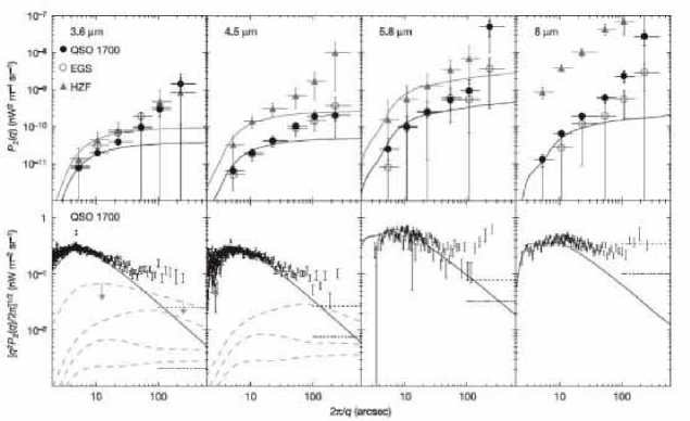
Figure 59: Detection of fluctuations in the infrared background from the analysis by Kashlinky et al (2005). The upper panel shows the angular power spectrum as a function of scale for 3 IRAC fields plotted for all four IRAC channels (3.6 through 8 $\mu$m). The solid line shows the effect of shot noise from the galaxy counts. This fits the fluctuations on small scales but there is a significant and consistent excess on large scales. Bottom panels refer to fluctuations for one IRAC field plotted as $(q^{2}P_{2}(q)/2\pi)^{\frac{1}{2}}$ with the predicted contributions from various populations of unresolved distant sources shown as dotted lines.

Kashlinksky et al argue that the excess signal is fairly flat spectrally in $\nu\,I_{\nu}$ ruling out any instrumental or Galactic contamination. The constancy of the signal over the wide range in Galactic latitude likewise suggests the signal is extragalactic. However, zodiacal light is difficult to eliminate as a contaminant. Although the signal persists when the Earth is 6 months further around in its orbit, no analysis of the likely zodi fluctuation spectrum is presented.

If the signal persists, what might it mean for sources fainter than 0.3 $\mu$Jy? Without a detailed redshift distribution, it is hard to be sure. The clustering pattern is remarkably strong given the depth of the imaging data (much deeper fields have subsequently been imaged but no independent analyses have yet been published). In summary, this is an intriguing result, somewhat unexplained and in need of confirmation

8.5 EBL Constraints from TeV Gamma Rays

High energy (TeV) gamma rays are absorbed in the earth’s atmosphere and converted into secondary particles forming an ‘air shower’. Cerenkov light is generated - a beam of faint blue light lasting a few $\times 10^{-9}$ sec is produced illuminating an area of 250m in diameter on the ground.

The significance of searching for TeV gamma rays is that they interact with the sea of 1-10 $\mu$m (infrared background) photons via the pair-creation process, viz:

$$\gamma\,\gamma\rightarrow e^{+}\,e^{-}$$

producing attenuation in distant sources (blazars) whose spectral energy distributions are assumed to be power laws.

$$\frac{d\,N}{d\,E}\propto E^{-\Gamma}$$

The strength of the attention, measured as a change in $\Gamma$, for the most distant accessible blazars is thus a measure of the degree of interaction between the gamma rays and the ambient infrared background.

The HESS team (Aharonian et al 2006) have recently analyzed the gamma ray spectrum of a blazar at $z$=0.186 and fitted its energy spectrum. As a result they can predict an upper limit to the likely infrared background for various assumptions (Figure 60). The constraint is most useful in the wavelength range 1-10$\mu$m where the associated gamma ray spectral data is of high quality (top axis of Fig. 60). This new method is intriguing. Although in detail the constraint is dependent on an assumed form for the TeV energy spectrum of blazars, for all reasonable assumptions the acceptable background is much lower at 1-4 $\mu$m than claimed by the traditional experiments.

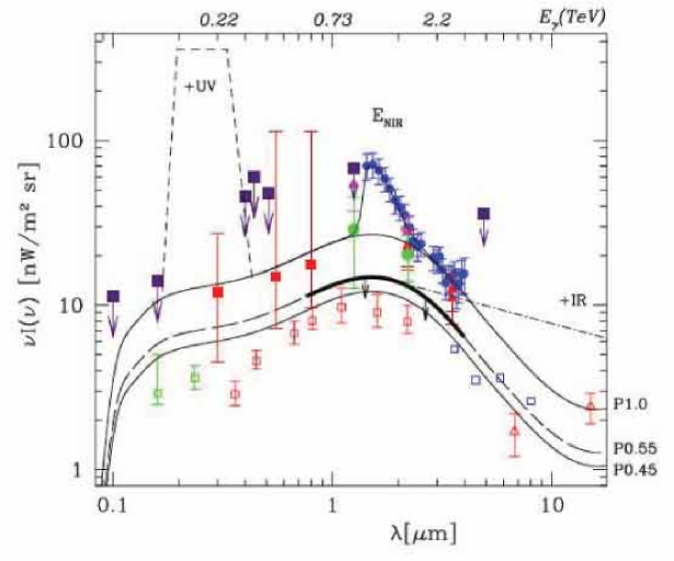
Figure 60: Constraints on the cosmic infrared background from the degree of attenuation seen in the high energy gamma ray spectrum of a distant blazar (Aharonian et al 2006). The black curves indicate likely upper limits to the infrared background for various assumptions. This independent method argues the near-IR detections by Matsumoto et al (2005, blue circles) and others are spurious.

8.6 Lecture Summary

In this lecture we have learned that extragalactic background light measurements in principle offer an important and unique constraint on undiscovered distant source populations.

However, the observations remain challenging and controversial because of instrumental effects, related to the precision of absolute calibrations, and dominant foregrounds. In the 1-5$\mu$m spectral regions positive detections in excess of extrapolations of the source counts have been reported. This is interesting because this is the wavelength range where an abundant and early population of faint, unresolved $z>$10 sources would produce some form of infrared background.

At the moment, the claimed detections at 1-5 $\mu$m appear unreasonably strong. Too many stars would be produced by the star formation associated with this background signal and recent ultrahigh energy spectra of distant blazars likewise suggest a much weaker infrared background.

IRAC is a particularly promising instrument for the redshift range 10$<z<$20 and fluctuation analyses offer a valuable independent probe of the background, although it is hard to interpret the results and compare them with the more traditional DC level experiments.

Despite the seemlingly chaotic way in which the subject of the cosmic extragalactic background light has unfolded in the past decade, it is worth emphasizing that the motivation remains a strong one. Any information on the surface brightness, angular clustering and redshift range of radiation beyond the detected source counts will be very valuable information ahead of the discoveries made possible by future generations of facilities.

9 Epilogue: Future Prospects

9.1 Introduction

The students attending this lecture course are living at a special time! During your lifetime you can reasonably confidently expect to witness the location of the sources responsible for cosmic reionization, to determine the redshift range over which they were active and perhaps even witness directly the ‘cosmic dawn’ when the first stellar systems shone and terminated the ‘Dark Ages’!

We have made such remarkable progress in the past decade, reviewed here, that such a bold prediction seems reasonable, even for a cautious individual like myself! We have extended our fundamental knowledge of how various populations of galaxies from 0$<z<$3 combine to give us a broad picture of galaxy evolution, while extending the frontiers to $z\simeq$7 and possibly beyond. Certainly many issues remain, including the apparent early assembly of certain classes of quiescent galaxy, the abundance patterns in the intergalactic medium and the apparent ‘downsizing’ signatures seen over a variety of redshifts. However, the progress has been rapid and driven by observations. Accompanying this is a much greater synergy between theoretical predictions and observations than ever before.

We have seen that the question of ‘First Light’ - the subject of this course - is the remaining frontier for observations of galaxy formation. The physical processes involved are poorly understood and thus observations will continue to be key to making progress. In this final lecture, I take out my crystal ball and consider the likely progress we can expect at optical and near-infrared wavelengths with current and near-term facilities ahead of those possible with the more ambitious new observatories such as the James Webb Space Telescope (JWST) and a new generation of extremely large ground-based telescopes.

9.2 The Next Five Years

Panoramic imaging with large optical and near-infrared cameras on telescopes such as Subaru, UKIRT and VISTA will enable continued exploration of the abundance of luminous drop-outs and Ly$\alpha$ emitters over 5$<z<$7, reducing the currently troublesome issues of cosmic variance. Deeper data will continue to be provided from further fields taken with ACS and NICMOS. With further spectroscopic surveys on large telescopes, we can expect improved stellar mass density estimates at $z\simeq$5-6 (Eyles et al 2006). However, strong gravitational lensing may still be the only route to probing intrinsically fainter sources, particularly beyond $z\simeq$7.

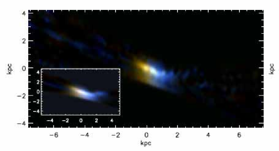
Figure 61: Detailed studies of a lensed $z\simeq$5 galaxy (Swinbank et al 2006). (Top) Reconstructed color HST VI image of the $z$=4.88 arc in the cluster RCS0224-002. The inset shows the effect of 0.8 arcsec seeing on the reconstruction, thereby demonstrating the advantage of lensing. In the source plane, the galaxy is 2.0$\times$0.8 kpc. (Bottom) [O II] velocity field obtained during a 12 hr VLT SINFONI exposure without AO. Spatial comparison with the Ly$\alpha$ field gives clear evidence of significant bi-polar outflows.

More detailed characterization of the properties of the most massive galaxies at $z\simeq$5-6 will also be worthwhile, in addition to continuing to deduce statistical properties such as abundances and luminosity functions.. Laser-guide star adaptive optics is now in widespread use on our 8-10 meter class telescopes and, with integral field spectrographs, can be used to probe the resolved dynamics of distant galaxies (Genzel et al 2006). Application of these techniques to the most intense star-forming lensed systems at $z>$4 (Swinbank et al 2006, Figure 61) is already providing unique insight into the physical state of the earliest galaxies. Extending the same techniques with adaptive optics will advance progress and address process on remarkably small scales ($\simeq$200 pc).

A number of special purpose ground-based instruments are also being developed, both with and without adaptive optics, to probe for $z>$7 dropouts and Lyman $\alpha$ emitters. These include:

• The Dark Age Z Lyman Explorer (DAZLE, Horton et al 2004), a moderate field (7 arcmin) infrared narrow-band imager with airglow discrimination whose goal is to reach a sensitivity of $\simeq 10^{-18}$ cgs in a night of VLT time. This corresponds to a limiting star formation rate of $\simeq 1M_{\odot}$ yr^-1 in quiet regions of the airglow spectrum at $z\simeq$7.7 and 9.9. Given the modest field and the need for dedicated spectroscopic follow-up, a long term campaign is envisaged to conduct a reliable census.

• The Gemini Genesis Survey (GGS ) which uses F2T2, a clone of the tunable filter destined for JWST (Scott et al 2006). This instrument is planned to work behind the Gemini Observatory’s multi-conjugate adaptive optics facility and image, in steps of wavelength, regions lensed by foreground clusters. The success of such a strategy will depend on both the angular size and line widths of $z>$7 Lyman $\alpha$ emitters and the abundance of intrinsically faint examples. Ellis et al (2001) found the lensed emitter at $z\simeq$5.7 was less than 30 milli-arcsec across with a line width of only 100-200 kms sec^-1. If such tiny emitters are the norm at $z>$7, the GGS may go much deeper than extant spectroscopic lensed searches (Stark et al 2006b).

The exciting redshift range 7$<z<12$ will also be the province of improved drop-out searches using the instrument WFC3 slated to be installed on Hubble Space Telescope in 2008-9. The infrared channel of this instrument spans 850 - 1170 nm with a field of $\simeq$ 2 arcmin at an angular resolution of 0.13 arcsec pixel^-1. This resolution is coarser than that of adaptive optics-assisted instruments such as F2T2. The principal gain over ground-based instruments will be in deep broad-band imaging free from airglow. The survey efficiency is about an order of magnitude better than that of NICMOS. WFC3 also has two infrared grisms which will be helpful in source discrimination.

A major stumbling block at the moment, even at $z\simeq$5-6, is efficient spectroscopic follow-up of dropout candidates. As we discussed in §6, photometric redshifts have unfortunately become de rigeur in statistical analyses of luminosity densities and luminosity functions (Bouwens et al 2006), yet their precision remains controversial. For z- and J-band dropous beyond $z\simeq$7, photometric redshifts will be even less reliable. Spitzer detections will be harder and fewer, and the typical source may have only 2-3 detected bands. Candidates may be found in abundance but how will they be confirmed?

The various 8-10m telescopes are now building a new generation of cryogenic near-infrared multi-slit spectrographs. It can be hoped that long exposures with these new instruments will be sufficient to break this impasse.

9.3 Beyond Five Years

A number of facilities are being planned, motivated by the progress discussed in these lectures. These include:

Figure 62: The 6.5m James Webb Space Telescope: Then (2013 in orbit) and and Now (2005, full scale model).

Figure 63: The proposed US-Canadian Thirty Meter Telescope (www.tmt.org) now in the detailed design phase.

• James Webb Space Telescope - a 6.5 meter optical-infrared space observatory (Gardner et al 2006) for which a primary mission is the detailed study of the earliest star-forming galaxies (Figure 62). The facility is currently planned to have a near-infrared imager NIRCam, a spectrograph NIRSpec with both integral field and limited multi-object modes, a tunable filter (as F2T2) and a mid-IR imager, MIRI. Stiavelli (2002) has presented a cogent summary of the likely strategies of using this facility, due to be launched in 2013, for studies of the earliest systems.

• Extremely Large Telescopes on the ground including the US-Canadian Thirty Meter Telescope (TMT, see www.tmt.org, Figure 63) which will have a diffraction-limited near-infrared imager/spectrograph (IRIS) and a adaptive-optics assisted spectrograph (IRMOS) with multiple deployable integral field units - area mapping units which can be arranged not only to scan regions surrounding luminous sources but also to undertake multi-object studies in crowded regions (Figure 64). At the time of writing, TMT is expected to be operational from 2016 onwards.

These will complement redshifted 21cm line tomography with radio facilities and address the key questions of the escape fraction of photons from star-forming sources and how they create ionized bubbles which merge to cause reionization.

It is quite likely that, by 2013, the redshift range containing the earliest galactic sources, estimated at present to be 10$<z<$20 perhaps, will have been refined sufficiently by special-purpose instruments on our existing 8-10 meter class telescopes. Thus one can surmise that that both JWST and future ELTs will be used for much more challenging work related to the physical process of reionization, as well as the chemical maturity of the most luminous sources found at high redshift.

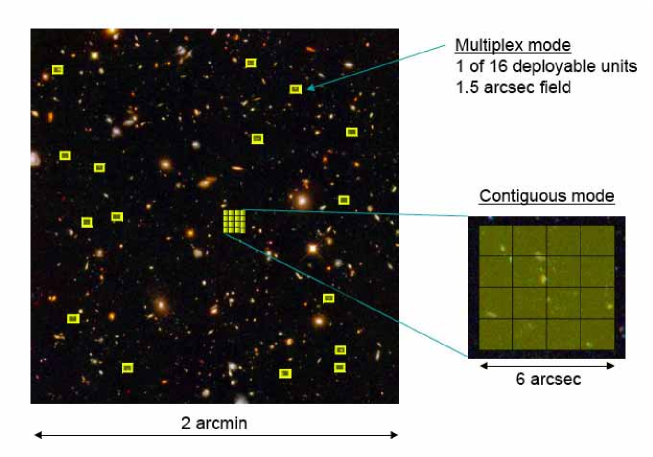
Figure 64: Flexibility in the deployment strategy for the multiple integral field units (yellow squares) for the proposed TMT infrared multi-object adaptive optics assisted instrument IRMOS. The IFUs can be distributed around the full field of 2 arcmin in classic multi-object mode. Alternatively, the IFUs can be configured together to map a small 6 $\times$ 6 arcsec field at high angular resolution in ‘blind’ mode. Such flexibility will be important in mapping Ly$\alpha$ emission at high redshift in various situations.

An obvious partnership between JWST and TMT, for example, which would complement the 21cm studies, would be to (i) search for the extent and topology of faint Ly$\alpha$ emission in ionized bubbles around JWST-selected luminous star forming galaxies and, (ii) pinpoint early sources for spectroscopic scrutiny so as to identify signatures of Population III stars.

At the present time there are so many imponderables in our knowledge of the earliest sources, that even the design parameters for the ELT instruments is a considerable challenge. How big are the faintest Ly$\alpha$ emitters? What are the typical line widths in km sec^-1? How big are the ionized bubbles at a given redshift? And, crucially, what is the surface density of various types of star-forming galaxies. Flexibility in the design of survey strategies will be crucial with instruments such as TMT’s IRMOS (Fig. 64).

Any information we can glean on the properties of $z\simeq$10 sources in the next 5 years will be valuable in optimizing how to move forward when these magnificent new generation telescopes are made available to us. Indeed, it is foolhardy to wait! Time and again, we can retrospectively look back at what we thought we would accomplish with our planned facilities and we always find that we achieved more than we expected!

10 Acknowledgements

I thank Daniel Schaerer, Denis Puy and Angela Hempel for inviting me to give these lectures in such a magnificent location with an enthusiastic group of students. I also thank my fellow lecturers, Avi Loeb and Andrea Ferrara and all of the foregoing for their patience in waiting for the completion of my written lectures. I thank my close colleagues Kevin Bundy, Sean Moran, Mike Santos and Dan Stark for their help and permission to show results in progress as well as Ivan Baldry, Jarle Brinchmann, Andrew Hopkins, John Huchra and Jean-Paul Kneib for valuable input. Finally, I thank Ray Carlberg and his colleagues for their hospitality of the Astronomy Department at the University of Toronto where the bulk of these lectures notes were completed.

11 References

Aaronson, M 1978 Ap J 221, L103

Aharonian, F. et al 2006 Nature 440, 1018

Adelberger, K et al 1998 Ap J 505, 18

Astier, P. et al 2006 Astron. Astrophys., 447, 31

Bahcall, N. et al 1999 Science 284, 1481

Baldry, I. & Glazebrook, K. 2003 Ap J 593, 258

Barkana, R. & Loeb, A 2000 Phys Rep. 349, 125

Baugh, C. et al 1996 MNRAS 283, 1361

Baugh, C. et al 1998 Ap J 498, 504

Baugh, C. et al 2005a MNRAS 305, L21

Baugh, C. et al 2005b MNRAS 356, 1191

Becker, G et al 2006 Ap J in press, (astro-ph/0607633)

Becker, R.H. et al 2001 AJ 122, 2850

Beckwith, S. et al 2006 AJ 132, 1179

Bell, E. et al 2004 Ap J 608, 752

Bell, E. et al 2006 Ap J 640, 241

Bender, R. et al 1992 Ap J 399, 462

Bennett, C. et al 2003 Ap J Suppl., 148, 97

Benson, A. et al 2002 MNRAS 336, 564

Benson, A. et al 2003 Ap J 599, 38

de Bernadis, P. et al 2000 Nature 404, 955

Bernstein, R. et al 2002 Ap J 571, 56

Blain, A. et al 2002 Phys. Rep. 369, 111

Blain, A. et al 2004 Ap J 611, 725

Blandford, R. & Narayan, R. 1992 ARAA 30, 311

Blanton, M.R. et al 2001 A.J. 121, 2358

Blumenthal, G. et al 1984 Nature 311, 517

Bolton, A. et al 2006 Ap J 638, 703

Bouwens, R. et al 2004 Ap J 606, L25

Bouwens, R. et al 2006 Ap J in press (astro-ph/0509641)

Bower, R. et al 1992 MNRAS 254, 601

Bower, R. et al 2006 MNRAS 370, 645

Brinchmann, J. & Ellis, R.S. 2000 Ap J 536, L77

Broadhurst, T. et al 1992 Nature 355, 55

Broadhurst, T. et al 2005 Ap J 621, 53

Bruzual, G. 1980 Ph.D. thesis, UC Berkeley

Bundy, K. et al 2004 Ap J 601, L123

Bundy, K. et al 2005 Ap J 625, 621

Bundy, K et al 2006 Ap J 651, 120

Bunker, A. et al 2004 MNRAS 355, 374

Bunker, A. et al 2006 New AR 50, 94

Calzetti, D. et al 2000 Ap J 533, 682

Caroll, S. et al 1992 ARAA 30, 499

Chabrier, G. 2003 PASP 115, 763

Chapman, S. et al 2003 Nature, 422, 695

Chapman, S. et al 2005 Ap J 622, 772

Conselice, C. et al 2005 Ap J 628, 160

Cowie, L. et al 1995 AJ 109, 1522

Cowie, L. et al 1996 AJ 112, 839

Cole, S. et al 2000 MNRAS 319, 168

Cole, S. et al 2001 MNRAS 326, 255

Cole, S. et al 2005 MNRAS 362, 505

Colless, M. et al 2001 MNRAS 328, 1039

Couch, W. et al 1998 Ap J 497, 188

Croton, D. et al 2006 MNRAS 365, 11

Daddi, E. et al 2004 Ap J 617, 746

Davies, R. L. et al 2001 Ap J 584, L33

de Lucia, G. et al 2006 MNRAS 366, 499

Dickinson, M. et al 2003 Ap J 587, 25

Dickinson, M. et al 2004 Ap J 600, L99

Djorgovski, S. & Davis, M. 1987 Ap J 313, 59

Djorgovski, S. et al 2001 Ap J 560, L5

Dole, H. et al 2006 Astron. Astrophys. 451, 417

Dressler, A. 1980 Ap J 236, 351

Dressler, A. et al 1987 Ap J 313, 42

Dressler, A.. et al 1997 Ap J 490, 577

Driver, S. et al 1995 Ap J 453, 48

Drory, N. et al 2005 Ap J 619, L131

Dube, R.R. et al 1979 Ap J 232, 333

Dunlop, J. et al 2006 MNRAS in press (astro-ph/0606192)

Ebbels, T. et al 1998 MNRAS 295, 75

Eddington, A.S. 1919 Obs. 42, 119

Egami, E. et al 2005 Ap J 618, L5

Erb, D. et al 2006 Ap J 644, 813

Ellis, R.S. 1997 ARAA 35, 389

Ellis, R.S. et al 1996 MNRAS 280, 235

Ellis, R.S. et al 2001 Ap J 560, L119

Ellison, S. et al 2000 AJ 120, 1175

Eyles, L. et al 2005 MNRAS 364, 443

Eyles, L. et al 2006 MNRAS, in press (astro-ph/0607306)

Fall, S. & Efstathiou, G. 1980 MNRAS 193, 189

Fall, S. et al 1996 Ap J 464, L43

Fan, X. et al 2003 AJ 125, 1649

Fan, X. et al 2006a ARAA 44, 415

Fan, X. et al 2006b AJ 132, 117

Felton, J. E. 1977, AJ 82, 861

Finkbeiner, D et al 2000 Ap J 544, 81

Fontana, A. et al 2004 Astron. Astrophys., 424, 23.

Franx, M. et al 2003 Ap J 587, L79

Frayer, D. et al 2000 AJ 120, 1668

Freedman, W. et al 2001 Ap J 553, 47

Fukugita, M. & Kawasaki, M. 2003 MNRAS 343, L25

Fukugita, M. & Peebles, P.J.E. 2004 Ap J 616, 643

Fukugita, M. et al 1998 Ap J 503, 518

Furlanetto, S. et al 2005 Phys. Reports 433, 181

Gardner, J. et al 2006 Space Sci. Rev. in press (astro-ph/0606175)

Genzel, R. et al 2006 Nature 442, 786

Gerhard, O. et al 2001 AJ 121, 1936

Giavalisco, M. et al 2004 Ap J 600, 103

Glazebrook, K. et al 1995 MNRAS 275, L19

Glazebrook, K. et al 2004 Nature 430, 181

Gradshteyn, I.S. & Ryzhik, I.M. 2000, Tables of Integrals, Series and Products, Academic Press

Granato, G.L. et al 2000 Ap J 542, 710

Gunn, J.E. & Peterson, B.A. 1965 Ap J 142, 1633

Haiman, Z. 2002 Ap J 576, 1

Hanany, et al 2000 Ap J 545, 5

Hauser, M & Dwek, E 2001 ARAA 39, 249

Hauser, M. et al 1998 Ap J 508, 25

Hoekstra, H. et al 2005 Ap J 647, 116

Hopkins, A.M. 2004 Ap J 615, 209

Hopkins, A.M. & Beacom, J. 2006 Ap J 651, 142

Horgan, J. 1998 The End of Science, Addison-Wesley

Horton, A. et al 2004 in Ground-based Instrumentation for Astronomy, S.P.I.E. 5492, 1022

Hu, E. et al 2004 AJ 127, 563

Hubble, E. 1936 The Realm of the Nebulae, Yale Univ. Press

Hughes, D. et al 1998 Nature 394, 241

Iye, M. et al 2006 Nature 443, 186

Jorgensen, I. et al 1996 MNRAS 280, 167

Jullo, E et al 2006, Astron. Astrophys, submitted

Juneau, S. et al 2005 Ap J 619, L135

Kaiser, N. et al 1987 MNRAS 277, 1

Kauffmann, G. & Charlot, S. 1998 MNRAS 297, L23

Kauffmann, G. et al 1993 MNRAS 264, 201

Kauffmann, G. et al 1996 MNRAS 283, L117

Kauffmann, G. et al 1999 MNRAS 303, 188

Kauffmann, G. et al 2003 MNRAS 341, 33

Kashikawa, N. et al 2006 Ap J 648, 7

Kashlinsky 2005 Phys. Reports 409, 361

Kashlinsky et al 2002 Ap J 579, 53

Kashlinsky et al 2005 Nature 438, 45

Kashlinsky et al 2006 Ap J Lett in press (astro-ph/0612445)

Kelsall, T. et al 1998 Ap J 508, 44

Kennicutt, R. 1983 Ap J 272, 54

Kennicutt, R. 1998 ARAA 36, 189

Kneib, J-P. et al 1996 Ap J 471, 643

Kneib, J-P. et al 2004 Ap J 607, 697

Kodaira, I. et al 2003 PASJ 55, L17

Kogut, A. et al 2003 Ap J Suppl., 148, 161.

Kong et al 2006 Ap J 638, 72

Koo, D. & Kron, R. 1992 ARAA 30, 613.

Koopmans, L. & Treu, T. 2003 Ap J 583, 606

Kriek, M. et al 2006 Ap J 649, L71

Kroupa, P. et al 1993 MNRAS 262, 545

Kroupa, P. 2001 MNRAS 332, 231

Lanzetta, K. et al 2002 Ap J 570, L492

Leinert, C. et al 1995 Astron. Astrophys. Suppl. 112, 99

Le Fevre, O. et al 2000 MNRAS 311, 565

Lilly, S.J. et al 1996 Ap J 460, L1

McCarthy, P. 2004 ARAA 42, 477

McCarthy, P. et al 2004 Ap J 614, L9

McClure, R. et al 2006 MNRAS 372, 357

Madau, P. & Pozzetti, L. 2000 MNRAS 312, L9

Madau, P. & Silk, J. 2005 MNRAS 359, L37

Madau, P. et al 1996 MNRAS 283, 1388

Madau, P. et al 1998 Ap J 498, 106

Madau, P. et al 1999 Ap J 514, 648

Maddox, S. et al 1990 MNRAS 242, 43

Malhotra, S. & Rhoads, J. 2004

Malhotra, S. et al 2005 Ap J 627, 666

Malin, D. & Carter, D 1980 Nature 285, 643

Mather, J. et al 1990 Ap J 354, 37

Mattilia, K. 1976 Astron. Astrophys. 47, 77

Mattila, K. 2003 Ap J 591, 119

Mattila, K. 2006 MNRAS 372, 1253

Matsumoto, T. et al 2005 Ap J 626, 31

Meier, D.L. 1976 Ap J 207, 343

Mellier, Y. 2000 ARAA 37, 127

Miller, G.E. & Scalo, J. 1979 Ap J Suppl. 41, 513

Miralda-Escude, J. et al 1998 Ap J 501, 15

Mobasher, B. et al 2005 Ap J 635, 832

Nagamine, et al 2004 Ap J 610, 45

Nagao, T. et al 2005 Ap J 634, 142

Newman J. & Davis, M 2000 Ap J 534, L11

Norberg, P et al 2002 MNRAS 336, 907

Oppenheimer, B.D. et al 2006 in Chemodynamics: First Stars to Local Galaxies, in press (astro-ph/0610808)

Ostriker, J. & Peebles, P. 1973 Ap J 186, 467

Ostriker, J & Steinhardt, P. 1996 Nature 377, 600

Ouchi, M. et al 2005 Ap J 620, L1

Papovich, C. et al 2006 Ap J 640, 92

Partridge, B. & Peebles, P.J.E. 1967 Ap J 147, 868

Peacock et al 2001 Nature 410, 169

Peebles, P. 1980 Large Scale Structure of the Universe, Univ. Chicago.

Penzias, A. & Wilson, 1965 Ap J 142, 419

Perlmutter, S. et al 1999 Ap J 517, 565

Pettini, M. et al 2002 Astrophys. Sp. Sci. 281, 461

Postman, M. et al 2005 Ap J 623, 721

Pritchet, C. 1994 PASP 106, 1052

Reddy, N. et al 2005 Ap J 633, 748

Refregier, A. 2003 ARAA 41, 645

Richard, J. et al 2006 Astron. Astrophys. 456, 861

Riess, A. et al 1995 AJ 116, 1009

Rowan-Robinson, M. 1985 The Cosmic Distance Scale (Freeman)

Rubin, V. 2000 PASP 112, 747

Rubin, V. et al. 1976 AJ 81, 687

Rudnick, G. et al 2003 Ap J 599, 847

Salpeter, E. 1955 Ap J 121, 161

Sand, D.J. et al 2005 Ap J 627, 32

Sandage, A. 2005 ARAA 43, 581

Santos, M. 2004 MNRAS 349, 1137

Santos, M. et al 2004 Ap J 606, 683

Sargent, M.T. et al Ap J in press (astro-ph/0609042)

Seitz, et al 1998 MNRAS 298, 945

Scalo, J. 1986 Fund. Cosmic Phys. 11, 1

Schechter, P. 1976 Ap J 203, 297

Schlegel, D. et al 1998 Ap J 500, 525

Schneider, P. 2006 in Gravitational Lensing: Strong, Weak & Micro, Saas-Fee Advanced Course 33

Scott, A. et al 2006 in Ground-based and Airborne Instrumentation for Astronomy, S.P.I.E. 6269, 176

Shapley, A. et al 2001 Ap J 562, 95

Shapley, A. et al 2003 Ap J 588, 65

Shapley, A. et al 2005 Ap J 626, 698

Shimasaku, K. et al 2005 PASJ 57, 447

Shioya Y. et al 2005 PASJ 57, 287

Smail, I. et al 1995 Ap J 440, 501

Smail, I. et al 1997 Ap J 490, L5

Smith, G. et al 2005 Ap J 620, 78

Smoot, G. et al 1992 Ap J 396, 1

Somerville, R. & Primack, J. 1999 MNRAS 310, 1087

Somerville, R. et al 2001 MNRAS 320, 504

Somerville, R. et al 2004 Ap J 600, L171

Songaila, A. 2004 AJ 127, 2598

Songaila, A. 2005 AJ 130, 1996

Songaila, A. 2006 AJ 131, 24

Spergel, D. et al 2003 Ap J Suppl. 148, 175

Spergel, D. et al 2006 Ap J in press (astro-ph/0603449)

Springel, V. et al; 2005 Nature 435, 629

Stanway, E. et al 2004 Ap J 607, 704.

Stanway, E. et al 2005 MNRAS 359, 1184

Stark, D. & Ellis, R.S. 2005 New AR 50, 46

Stark, D. et at 2006a Ap J in press (astro-ph/0604250)

Stark, D. et al 2006b Ap J submitted

Stiavelli, M. 2002 in Future Research Directions & Visions for Astronomy, S.P.I.E. 4835, 122

Stiavelli, M. et al 2004 Ap J 600, 508

Steidel, C. et al 1996 Ap J 492, 428

Steidel, C. et al 1999a Ap J 519, 1

Steidel, C. et al 1999b Phil Trans R. Soc. 357, 153

Steidel, C. et al 2003 Ap J 592, 728

Struck-Marcell, & Tinsley, B. 1978 Ap J 221, 562

Sullivan, I. et al 2006 Ap J in press (astro-ph/0609451)

Sullivan, M. et al 2000 MNRAS 312, 442

Sullivan, M. et al 2001 Ap J 558, 72

Swinbank, M. et al 2006 Ap J submitted

Taniguchi, Y. et al 2005 PASJ 57, 165

Tinsley, B. 1980 Fund. Cosmic Phys. 5, 287

Toomre, A. & Toomre, J 1972 Ap J 178, 623

Tran, K.-V. et al 2005 Ap J 627, L25

Treu, T. et al 2005 Ap J 622, L5

Treu, T et al 2006 Ap J 640, 662

Tully, B. & Fisher, 1977 Astron. Astrophys. 54, 661

van der Wel, A. et al 2005 Ap J 631, 145

van der Wel, A. et al 2006 Ap J 636, L21

van Dokkum, P. 2005 AJ 130, 2647

van Dokkum, P. & Ellis, R.S. 2003 Ap J 592, L53

van Dokkum, P. et al 2003 Ap J 587, L83

van Dokkum, P. et al 2006 Ap J 638, L59

Vogt, N. et al 1996 Ap J 465, L15

Vogt, N. et al 1997 Ap J 479, L121

Weiner, B. et al 2005 Ap J 620, 595

Wright, E. & Reese, E.D. 2000 Ap J 545, 43

Yan, H. & Windhorst, R. 2004 Ap J 612, 93

Yan, H. et al 2005 Ap J 634, 109

Yan, H. et al 2006 Ap J 651, 24

Yee, H. et al 1996 AJ 111, 1783

York, D. et al 2001 AJ 120, 1579

Zwaan, M.A. et al 2003 AJ 125, 2842

Zwicky, F. 1933 Helv. Physica Acta, 6, 110

Zwicky, F. 1937 Phys Rev. 51, 290