Dynamical masses of ultra-compact dwarf galaxies in Fornax

Abstract

Aims. We determine masses and mass-to-light ratios of five ultra-compact dwarf galaxies and one dwarf elliptical nucleus in the Fornax cluster from high resolution spectroscopy. We examine whether they are consistent with pure stellar populations or whether dark matter is needed to explain their masses.

Methods. Velocity dispersions were derived from selected wavelength regions using a direct-fitting method. To estimate the masses of the UCDs a new modelling program has been developed that allows a choice of different representations of the surface brightness profile (i.e. Nuker, Sersic or King laws) and corrects the observed velocity dispersions for observational parameters (i.e. seeing, slit size). The derived dynamical masses are compared to those expected from stellar population models.

Results. The observed velocity dispersions range between 22 and 30 km s^-1. The resulting masses are between 1.8 and $9.5\times 10^{7}M_{\odot}$. These, as well as the central and global projected velocity dispersions, were derived from the generalized King model which turned out to give the most stable results. The masses of two UCDs, that are best fitted by a two-component profile, were derived from a combined King+Sersic model. The mass-to-light ratios of the Fornax UCDs range between 3 and 5 $(M/L_{V})_{\odot}$. The $M/L_{V}$ ratio of the dwarf elliptical nucleus is 2.5. These values are compatible with predictions from stellar population models. Within 1-2 half-mass radii dark matter is not dominating UCDs and the nucleus. An increasing dark matter contribution towards larger radii can not be ruled out with the present data. The $M/L_{V}$ ratios of some UCDs suggest they have intermediate age stellar populations.

Conclusions. We show that the mass-to-light ratios of UCDs in Fornax are consistent with those expected for pure stellar populations. Thus UCDs seem to be the result of cluster formation processes within galaxies rather than being compact dark matter dominated substructures themselves. Whether UCDs gained their mass in super-star cluster complexes of mergers or in nuclear star cluster formation processes remains an open question. It appears, however, clear that star clusters more massive than about $5\times 10^{6}M_{\odot}$ exhibit a more complex formation history than the less massive ‘ordinary’ globular clusters.

1 Introduction

In the late 1990s a new type of very bright compact stellar system was discovered in the core of the nearby Fornax galaxy cluster (Hilker et al. hilk99c (1999), Drinkwater et al. drin00a (2000)). On ground-based images with typical resolution ($\sim 0.8$ arcsec seeing) these objects look like stars since at Fornax distance globular clusters (GCs) are unresolved. However, with absolute magnitudes in the range $M_{V}=-13.5$ to $-12.3$ they are about 2 mag brighter than $\omega$ Centauri, the most massive globular cluster in the Milky Way, but about 3 mag fainter than the compact dwarf elliptical M32. Their luminosities are comparable to those of nuclei of dwarf ellipticals or late-type spirals (i.e. Lotz et al. lotz04 (2004), Walcher et al. walc05 (2005), Côté et al. cote06 (2006)). Their sizes range between 10 and 30 pc in half-light radii (Drinkwater et al. drin03a (2003)) which is about 10 times larger than ordinary GCs.

Table 1: Observation log and properties of observed objects. $V_{0}$ is from Evstigneeva et al. (evst06 (2006)) and $(V-I)_{0}$ from Mieske et al. (mies06 (2006)) (except $(V-I)_{0}$ for FCC303 which is from Karick et al. kari03 (2003)). Both, $V_{0}$ and $(V-I)_{0}$ are corrected for foreground dust extinction (Schlegel et al. schl98 (1998)). The [Fe/H] values are from Mieske et al. (mies06 (2006)).

Name	FCSSa name	$\alpha$(2000)	$\delta$(2000)	$V_{0}$	$(V-I)_{0}$	[Fe/H]	Date	Exp. time	Seeing	S/Nb	S/Nb
		[h:m:s]	[∘:$\arcmin$:$\arcsec$]	[mag]	[mag]	[dex]		[s]	[$\arcsec$]	4900$\AA$	5900$\AA$
FCC303c		3:45:14.10	$-$36:56:12.0	15.90	1.09		2000 Dec 20	$3\times 1004$	0.80	3.6	4.2
UCD2	J033806.3$-$352858	3:38:06.33	$-$35:28:58.8	19.12	1.14	$-$0.90	2000 Dec 23	$5\times 1800$	0.55	4.5	5.6
UCD3	J033854.1$-$353333	3:38:54.10	$-$35:33:33.6	17.82	1.22	$-$0.52	2000 Dec 20	$3\times 1000$	0.80	4.7	5.9
UCD4	J033935.9$-$352824	3:39:35.95	$-$35:28:24.5	18.94	1.13	$-$0.85	2000 Dec 24	$5\times 1800$	0.60	4.8	5.6
UCD5	J033952.5$-$350424	3:39:52.58	$-$35:04:24.1	19.40	1.00		2001 Feb 12	$2\times 3285$	0.60	4.4	5.2
UCD5							2001 Feb 13	$2\times 3285$	0.55	4.8	5.8
UCD5							2001 Aug 19	$1\times 3285$	0.55	4.6	5.1
UCD5							2001 Sep 20	$1\times 3119$	0.80	5.3	6.3
UCD5							2001 Nov 19	$1\times 3285$	0.85	5.2	6.4

^aFornax Cluster Spectroscopic Survey (Drinkwater et al. drin99 (1999)); ^bmeasured for a single spectrum per resolution element ($=0.03$Å); ^cFornax Cluster Catalog (Ferguson ferg89a (1989))

In the last years, extensive surveys in the Fornax and Virgo cluster have revealed dozens of these compact objects (UCDs and bright GCs) in the magnitude range $-13.5<M_{V}<-11.0$ (i.e. Mieske et al. mies02 (2002) and mies04a (2004), Haşegan et al. hase05 (2005), Jones et al. jonej06 (2006)). They were dubbed ”ultra-compact dwarf galaxies” (UCDs) by Phillipps et al. (phil01 (2001)), and ”dwarf-globular transition objects” (DGTOs) by Haşegan et al. (hase05 (2005)), expressing their uncertain origin. Various formation scenarios have been suggested to explain the origin of UCDs. The most promising are:

1) UCDs are the remnant nuclei of galaxies that have been significantly stripped in the cluster environment (i.e. Bassino et al. bass94 (1994), Bekki et al. bekk03b (2003)). This would mean that UCDs once resided in the centres of dark matter (DM) dominated cosmological substructures. The isolated nuclei themselves, however, are probably not DM dominated since DM halos of galaxies can be stripped (Bekki et al. bekk03b (2003)). Moreover, present-day nuclei of dwarf ellipticals are dominated by their stellar populations, not by dark matter (Geha et al. geha02 (2002)).

2) UCDs formed from the agglomeration of many young, massive star clusters that were formed during merger events (i.e. Kroupa krou98 (1998), Fellhauer & Kroupa fell02a (2002)). Hence, UCDs would be dark matter free stellar objects that were not created in the centres of galaxies.

3) UCDs are the brightest globular clusters formed in the same GC formation event as their less massive counterparts (i.e. Mieske et al. mies02 (2002), Martini & Ho martin04 (2004)). Also in this case, UCDs would be objects possessing pure stellar populations.

4) UCDs are the surviving counterparts of genuine compact dwarf galaxies that formed in small dark matter halos at the low mass end of cosmological sub-structure (i.e. Drinkwater et al. drin04 (2004)). Nowadays UCDs survived the galaxy cluster formation and evolution processes, e.g. they were not disrupted or accreted by larger galaxies until the present time. This would mean that they might still be dominated by dark matter.

To distinguish the different formation scenarios one needs to study the detailed properties of UCDs, like structural parameters, internal kinematics, together with ages and chemical compositions of their stellar population(s). In particular, the internal velocity dispersion $\sigma_{0}$ of the stars within the UCDs is of interest, from which masses and mass-to-light ($M/L$) ratios can be estimated. A high virial $M/L$ ratio would imply a compact cosmological progenitor rather than a merged stellar super-cluster.

Recent high spatial resolution imaging and mid- to high-resolution spectroscopy shed some light on the properties of UCDs. First results on the velocity dispersion of UCDs in Fornax were presented in Drinkwater et al. (drin03a (2003)). These were based on a quick analysis of the same high resolution spectra that are the basis for this paper. The observed, projected velocity dispersions ranged between 24 and 37 km s^-1. Using the sizes of the UCDs – derived from high resolution surface brightness profiles – their masses and mass-to-light ratios ($M/L_{V}$) were roughly estimated. $M/L_{V}$ values were of the order 2-4 in solar units. This is slightly higher than the $M/L$ ratio of globular clusters, but much lower than that of dwarf spheroidal galaxies of similar mass. In the present paper, we revise the formerly obtained masses and $M/L$ ratios of the Fornax UCDs.

In the Virgo cluster, Haşegan et al. (hase05 (2005)) derived masses and $M/L$ ratios for six DGTOs/UCDs. Three of those have relatively high $M/L_{V}$ values between 6 and 9 at velocity dispersions between 20 and 30 km s^-1. This makes them the first UCDs with some evidence for dark matter, given their rather low metallicities ($-1.5<$[Fe/H]$<-0.7$ dex). Fellhauer & Kroupa (fell06 (2006)), however, point out that the tidal “heating” due to a close passage of an UCD through the central region of its host galaxy (pericenter between 100 and 1000pc) may lead to an overestimation of its virial mass at all orbital radii due to the presence of unbound stars in the line of sight. The effect would occur mostly for UCDs with nearly radial orbits. Such orbits are indeed predicted for the remnant nuclei of stripped galaxies (Bekki et al. bekk03b (2003)) because of the selective way tidal stripping works.

Figure 1: The six template spectra (see Table 2) are shown in 100$\AA$ wide regions around the H$\beta$ line ($\sim 4860\AA$, left panels) and the Na I doublet ($\sim 5890\AA$, right panels). The spectra are ordered by increasing metallicity as indicated.

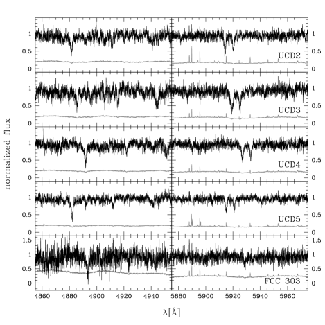
Figure 2: The five object spectra (see Table 1) are shown in 100$\AA$ wide regions around the H$\beta$ line ($\sim 4885\AA$, left panels) and the Na I doublet ($\sim 5920\AA$, right panels). The 1-sigma error are plotted as well (grey lines).

Table 2: Observation log and properties of standard stars that were used as velocity dispersion templates. They are ordered by their increasing metallicity. Most of the properties were taken from the SIMBAD database, see: http://simbad.u-strsbg.fr/Simbad

#	Name	Typea	$\alpha$(2000)	$\delta$(2000)	$V$	$(B-V)$	[Fe/H]	$v_{\rm helio}$	Date	Exp.	S/Nb	S/N
			[h:m:s]	[∘:$\arcmin$:$\arcsec$]	[mag]	[mag]	[dex]	[km s-1]		[s]	4900$\AA$	5900$\AA$
1	HD 21022	G	03:22:21.59	-32:59:39.7	9.20	0.95	$-$1.99	110$\pm$3	2000 Dec 20	50	50.0	55.0
2	HD 9051	G	01:28:46.47	-24:20:25.3	8.93	0.82	$-$1.50	$-$73$\pm$1	2000 Dec 20	40	52.0	57.0
3	HD 41667	G	06:05:03.64	-32:59:39.3	8.53	1.01	$-$1.18	302$\pm$10	2000 Dec 23	30	49.0	53.0
4	HD 20038	G	03:10:26.81	-58:49:40.5	8.90	0.84	$-$0.87	27$\pm$10	2000 Dec 24	40	52.0	55.0
5	HD 17233	SG	02:43:52.03	-54:47:28.3	9.03	0.79	$-$0.60	$-$18$\pm$10	2001 Feb 13	45	49.0	53.0
6	HR 296-1	K0III	01:03:02.50	-04:50:12.0	5.43	1.11	$-$0.14	15$\pm$?	2001 Aug 19	5	58.0	61.0
7	HR 296-2								2001 Sep 20	5	59.0	62.0
8	HR 296-3								2001 Nov 19	2.5	53.0	57.0

^aG: giant; SG: supergiant; ^bmeasured for a single spectrum per resolution element ($=0.03\AA$)

The structural parameters of the brightest Virgo and Fornax UCDs were presented in several recent papers (i.e. Haşegan et al. hase05 (2005), De Propris et al. depr05 (2005), Evstigneeva et al. evst06 (2006)). A striking result is that UCDs brighter than $M_{V}=-11.5$ follow a luminosity-size relation (Haşegan et al. hase05 (2005), Richtler rich06 (2006), Kissler-Patig et al. kiss06 (2006), Mieske et al. mies06 (2006)), different from the luminosity independent sizes of globular clusters (i.e. Jordán et al. jord05 (2005)). Moreover, the light profiles of the brightest UCDs cannot be described by a simple King profile (Evstigneeva et al. evst06 (2006)). Most of them show a cuspy profile in their centres and no tidal truncation within the observed surface brightness limit. Some of them exhibit small envelopes with effective radii upto 100 pc (e.g. Drinkwater et al. drin03a (2003); Richtler et al. rich05 (2005)).

Concerning the chemical abundances of UCDs, recent work suggests that most of the bright Virgo UCDs are old and have metallicities ranging from [Z/H]$=-1.35$ to $+0.35$ dex with an [$\alpha$/Fe] value of $\simeq$0.3 (Evstigneeva et al. evst06 (2006)), whereas the brightest Fornax UCDs are predominantly metal-rich ([Fe/H]$\simeq-0.5\pm 0.5$ dex; Mieske et al. mies06 (2006)). Their ages and $\alpha$-abundances are not constrained very well. Future surveys will clarify whether some UCDs may exhibit intermediate-age stellar populations.

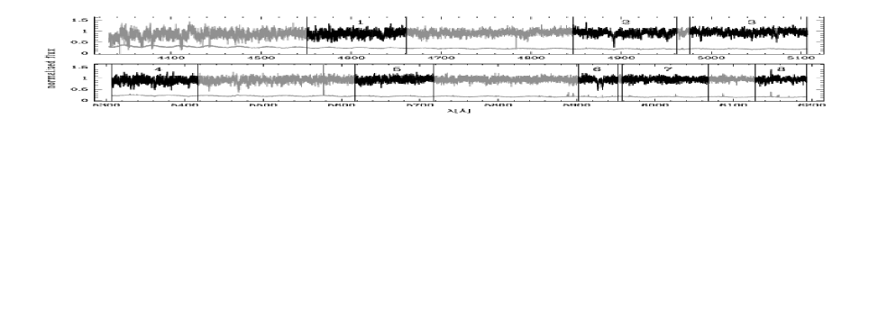
Figure 3: The “blue” part (upper panel) and the “red” part (lower panel) of the spectrum of UCD4 are shown. Dark regions mark the eight direct fitting regions for velocity dispersion measurements (see Table 3). The grey wavy lines are the 1-sigma error spectra.

In this paper, we determine dynamical masses of five of the brightest UCDs and one nucleus of a dwarf elliptical in the Fornax cluster. The work is based on the detailed analysis of high resolution spectroscopy that was obtained with the Very Large Telescope Ultraviolet and Visual Echelle Spectrograph (VLT/UVES) at Paranal/Chile (and Keck spectroscopy for one of the UCDs). The derivation of structural parameters for the UCDs – which are necessary to estimate virial masses – are taken from Evstigneeva et al. (evst06 (2006)). In section 2 of the present paper, the observations and data processing are described. Section 3 is dedicated to the velocity dispersion measurements, and section 4 to the derivation of masses and mass-to-light ratios by dynamical modelling and their comparison with expected values from stellar population models. Finally, in section 5 the main results are summarized. Throughout the paper we use a distance modulus of 31.39 mag for the Fornax cluster (Freedman et al. freed01 (2001)).

2 Observations and data reduction

2.1 Observations

The observations were performed between December 2000 and November 2001 with the VLT/UT2 at Paranal (ESO, Chile) in service mode. The instrument in use was the Ultraviolet and Visual Echelle Spectrograph (UVES), and an array of two attached 2$\times$4 k CCD chips. The data were read out with a 2$\times$2 binning, resulting in a spatial scale of 0.36″/pixel. The setting used (RED arm, $\lambda_{\rm central}=5200\AA$) provided a wavelength coverage of 4200-6200$\AA$, with a gap between 5160 and 5240$\AA$ (blind region beween the two CCD chips). The slit was chosen to have a width of 1″which gives a resolving power of 37000-45000. The final resolution ranged between 2.4 and 3.1 pixels (or 0.12 and 0.16$\AA$). It depends on the seeing which varied between $0\aas@@fstack{\prime\prime}5$ and $0\aas@@fstack{\prime\prime}9$.

Table 3: Wavelength regions for direct fitting of velocity dispersions and prominent lines therein. The values are given in the restframe.

Id	$\lambda_{\rm start}$	$\lambda_{\rm end}$	Absorption lines
	[$\AA$]	[$\AA$]
1	4523.2	4632.7	MgI4571
2	4816.8	4931.3	CIV, H$\beta$
3	4946.2	5075.6	Fe5041
4	5274.6	5384.1	Fe5371
5	5583.1	5682.6
6	5866.8	5916.5	NaI (D2), NaI (D1)
7	5921.5	6031.0
8	6090.7	6155.4	CaI1, CaI2

In total, four ultra-compact dwarfs in the magnitude range $17.8<V<19.4$ mag and one nucleus of a dwarf elliptical ($V_{\rm nuc}\simeq 19.5$) were observed. Most of the observations were taken in three nights in December 2000. Only for one object (UCD5), the single exposures were taken in five different nights between February and November 2001. The total integration time for the UCDs varied between 50 minutes and 6 hours. Table 1 gives a short logbook of the observations, together with the achieved S/N at two different wavelengths (per 0.05$\AA$ pixel). Also the properties of the observed objects are summarized in this table.

In the same run, spectra of six standard stars were taken with the same instrument configuration. They mostly are giants and cover a metallicity range of $-2.0<$[Fe/H]$<-0.1$ dex. Their properties are summarized in Table 2, and excerpts of their spectra around the H$\beta$ line and the Na doublet are shown in Fig. 1. The same spectral regions (however redshifted) for the UCDs and FCC303 are shown in Fig. 2.

2.2 Data reduction

The European Southern Observatory (ESO) provides pipeline reduced data for UVES echelle spectroscopy. The UVES context in the MIDAS environment is used for that reduction. Due the low S/N of our data, the pipeline reduced data with standard settings can not be trusted right away. Therefore, we decided to re-reduce these data with the same pipeline, carefully controlling all steps and optimizing the setup parameters. Also, we implemented a different more reliable cosmic ray removal routine as the one used by the pipeline.

The first steps, namely first guess solution, defining of order positions, wavelength calibration, were performed with the default settings of the UVES pipeline. Then, before the order tracing and extraction of the spectra, the cosmic rays in the low S/N science exposures were rejected by the LACOSMIC (Laplacian Cosmic Ray Identification) routine from van Dokkum (vando01 (2001)) which worked very well. This was necessary to avoid jumps in the tracing as a result of cosmic rays close to the spectra. For the further reduction, the inter-order background subtraction method MEDIAN, the OPTIMAL extraction, flatfield correction in the extracted pixel-order space, sky subtration, and merging of overlapping orders were chosen. Also an error spectrum containing the standard deviation of the reduced spectra was extracted for each object.

Since some spectra of the same object were observed at very different dates, a correction for the heliocentric velocity was necessary before combination. For UCD5, the heliocentric corrections differed by 35.08 km s^-1 between individual exposures. Since the instrumental spectral resolution is about 0.03$\AA$/pixel, a noticable shift in wavelength (10% $=$ 0.003$\AA$) already occurs for a velocity difference of $\geq 0.15$ km s^-1. The combination was done with the scombine under the noao.imred.echelle package of IRAF. Prior to averaging the single spectra they were scaled by their mode, and pixel values deviating more than 3 sigma from the average were rejected. In the same step the spectra were rebinned to a resolution of 0.05 $\AA$/pixel. The averaging and rebinning increased the S/N of a resolution element to 11-19 for the UCDs, depending on the object and the wavelength (see Table 4).

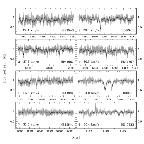
Figure 4: The direct fitting regions for the spectrum of UCD4 are shown (grey lines) together with the best fitting template (black lines). The name of the template, the velocity dispersion of the gaussian kernel and the number of the direct fitting region are indicated in each panel.

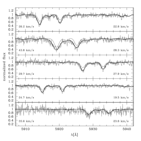
Figure 5: The Na doublet region for the five studied objects is shown (UCD2, UCD3, UCD4, UCD5 and FCC303 from top to bottom). The bold lines are averages of the three best-fitting templates for this region (region 6, see Table 3). The corresponding velocity dispersions are given on the left. Thin lines represent the averages of the three best-fitting templates in the regions 4, 5 and 7. Their velocity dispersions are given on the right.

Table 4: Results of velocity dispersion measurements in all direct fitting regions (same identification numbers as in Table 3). On the left, the results from the blue part of the spectrum are shown, and on the right the ones from the red part. The identification numbers of the three best fitting templates are given in brackets below each $\sigma_{v}$ value. The S/N are those for the combined spectra at the given wavelength.

Name	S/N	$\sigma_{v}$ [km s-1]				S/N	$\sigma_{v}$ [km s-1]
	4900$\AA$	1	2	3	1+2+3	5900$\AA$	4	5	6	7	8	4+5+7
UCD2	14.3	24.4$\pm$1.5	24.8$\pm$1.5	24.7$\pm$1.4	25.3$\pm$0.8	15.9	22.5$\pm$1.7	22.8$\pm$2.3	26.5$\pm$1.7	24.3$\pm$3.0	19.4$\pm$2.0	24.4$\pm$1.2
		(3,4,5)	(5,4,3)	(8,4,3)	(3,4,5)		(6,5,4)	(3,5,8)	(8,2,5)	(6,4,3)	(8,4,5)	(8,4,3)
UCD3	11.3	23.4$\pm$1.2	25.8$\pm$1.1	26.1$\pm$1.0	25.4$\pm$0.7	13.0	29.2$\pm$1.4	29.6$\pm$2.0	44.3$\pm$1.6	26.8$\pm$3.0	32.3$\pm$2.6	30.0$\pm$1.1
		(8,3,4)	(5,7,4)	(8,5,4)	(8,5,4)		(7,5,3)	(5,8,3)	(2,8,5)	(6,3,4)	(8,5,4)	(7,3,4)
UCD4	14.9	27.6$\pm$1.9	30.1$\pm$1.7	27.5$\pm$1.6	29.3$\pm$1.0	15.9	29.4$\pm$2.1	26.4$\pm$2.1	30.2$\pm$1.8	29.2$\pm$7.9	31.1$\pm$3.2	31.3$\pm$1.6
		(8,4,3)	(4,5,3)	(4,5,2)	(3,4,5)		(3,5,8)	(3,2,1)	(2,5,8)	(6,5)	(5,3,4)	(3,8,4)
UCD5	17.6	24.1$\pm$1.8	26.7$\pm$1.9	23.5$\pm$1.5	25.4$\pm$1.0	19.1	20.1$\pm$1.7	19.0$\pm$1.8	23.8$\pm$1.9	20.3$\pm$2.7	23.1$\pm$4.6	20.7$\pm$1.1
		(3,4,5)	(3,4,2)	(3,4,2)	(3,4,5)		(3,4,1)	(4,5,3)	(6,1,2)	(7,4,3)	(4,8,5)	(4,3,8)
FCC303	7.1	19.9$\pm$5.3	24.7$\pm$2.8	26.8$\pm$2.2	29.6$\pm$1.8	9.3	24.4$\pm$2.6	23.3$\pm$2.7	34.0$\pm$4.0	6.5$\pm$3.9	31.6$\pm$6.8	28.1$\pm$2.1
		(3,2,1)	(4,2,5)	(2,4,5)	(3,4,2)		(4,8,5)	(3,5,7)	(4,5,8)	(3,2,6)	(5,4,3)	(3,4,2)

The standard star spectra have a high S/N ($\sim 50$-60) and were reduced with the standard settings of the pipeline. They were rebinned to the same resolution as the science spectra.

3 Velocity dispersion measurements

The kinematic analysis of the spectra was performed using van der Marel’s direct-fitting method (van der Marel & Franx vdma93 (1993)). First, the spectra were placed on a logarithmic wavelength scale and normalized. Then, the standard star spectra were convolved with Gaussian velocity dispersion profiles in the range 2 to 60 km s^-1 and a step size of 1 km s^-1.

For the comparison of the templates with the UCD spectra, wavelength regions with prominent absorption features were selected. The restframe wavelengths of the direct fitting regions and some prominent lines they cover are summarized in Table 3 and are shown in Fig. 3. Additionally, direct fitting on a combination of three selected regions was performed for the bluer part (regions 1, 2 and 3) as well as for the redder part (regions, 4, 5 and 7) of the spectrum. All object spectra (UCDs and FCC 303) were fitted with all sets of smoothed template spectra (see Table 2). The best-fitting Gaussian velocity dispersion profile is determined by $\chi^{2}$ minimization in pixel space. As an example, the best fits to the spectrum of UCD4 for the eight direct fitting regions are shown in Fig. 4. In Table 4 the results for the three best-fitting templates (average values) are given for all fitting regions. The identification numbers of the three templates are given in brackets. In most cases, the derived velocity dispersions of these templates are consistent with each other within $\pm 2$ km s^-1. The template star HR296 was observed in three different nights. The velocity dispersions as derived from the three individual velocity dispersion fits with this star agree within $\pm 1$ km s^-1 with each other in all cases. Thus no systematic effects larger than $\pm 2$ km s^-1 either due to the use of different templates or observations in different nights are expected. The internal velocity dispersions of the stars are expected to be below 3 km s^-1, and thus do not affect the velocity dispersion measurements. Note that one resolution element of 0.05$\AA$/pixel corresponds to 2.5-3.5 km s^-1.

The best-fitting templates are in most cases the ones with metallicities between $-1$ and 0 dex. This should be expected since line index measurements of the Fornax UCDs 2, 3 and 4 revealed iron abundances of [Fe/H]$=-0.90$, $-$0.52 and $-$0.85 dex, respectively (Mieske et al. mies06 (2006)).

The scatter of velocity dispersion measurements between the different direct fitting regions is very different for the bluer and redder part of the spectrum. Whereas in the bluer part the scatter is of the order $\pm 1.5$ km s^-1, the regions 6 and 8 of the redder part, which include the Na doublet and a Ca line, reveal large discrepancies towards high $\sigma_{v}$ values. This effect is illustrated in Fig. 5 where the best fit to the Na doublet region is compared to the expected fit in this region when taking the average $\sigma_{v}$ of regions 4, 5 and 7. This discrepancy cannot easily be explained. Probably abundance mismatches and/or stellar population mixes play a role. The $\alpha$-abundances of UCDs in Virgo are known to have super-solar values (Evstigneeva et al. evst06 (2006)). One might also speculate whether the extra absorption might be caused by intra-cluster material in the line of sight. Future studies shall clarify this issue.

Table 4 also shows that there seems to exist a slight systematic effect between the velocity dispersion measurements in the bluer and redder part of the spectrum (excluding regions 6 and 8) for some objects. UCD3 has systematically higher $\sigma$ values in the red part as compared to the blue part, whereas for UCD5 the contrary is the case. Also here, template mismatches and contribution of stars from different evolutionary stages might be the reason.

To define a final velocity dispersion for each object we consider three cases of averaging the individual values: 1) simply the mean of all fits; 2) the mean of all fits but with a 2-sigma clipping of outliers; 3) mean excluding the Na and Ca region as well as the combined regions. The results are listed in Table 5. They are consistent with each other within the errors. We adopt the average velocity dispersion of case 2) as final value for further analyses.

Table 5: Average values for radial velocity and velocity dispersion measurements: (1) - mean of all fits; (2) - as (1), but with 2-sigma clipping; (3) - mean excluding Na and Ca region and combined region. The values in bold face are those used for further analyses. The velocity dispersion of UCD1 was derived by Drinkwater et al. (drin03a (2003)) from Keck spectroscopy.

Name	vhelio	$\sigma_{v}$	$\sigma_{v}$	$\sigma_{v}$
	[km s-1]	[km s-1]	[km s-1]	[km s-1]
		(1)	(2)	(3)
UCD2	1205.7$\pm$0.8	24.4$\pm$1.6	24.7$\pm$1.0	24.1$\pm$1.0
UCD3	1448.3$\pm$1.5	27.6$\pm$4.9	26.6$\pm$2.3	26.2$\pm$2.2
UCD4	1839.8$\pm$3.8	29.3$\pm$1.7	29.2$\pm$1.5	28.4$\pm$2.0
UCD5	1245.4$\pm$2.1	22.9$\pm$2.6	22.9$\pm$2.6	22.4$\pm$2.9
FCC303	1928.6$\pm$3.1	26.1$\pm$5.6	27.1$\pm$3.1	23.1$\pm$6.0
UCD1	…	…	32.0$\pm$1.0	…

For UCD1 no UVES spectroscopy is available. Yet its observed velocity dispersion is known from Keck spectroscopy (Drinkwater et al. drin03a (2003)). It was derived from the CaT region using a cross-correlation method (Tonry & Davis tonr79 (1979), as implemented in RVSAO/IRAF) and only one stellar template (G6/G8IIw type). The determined value is given in Table 5 and is used for the mass modelling (see next section). Note that in Drinkwater et al. (drin03a (2003)) also the velocity dispersions of UCD2 to UCD5 and FCC303 were determined via the cross-correlation method. Since in this preliminary study only the Na doublet region was used the obtained velocity dispersions are 2-10 km s^-1 higher than the adopted values of the present study (see discussion on the Na doublet above).

4 Mass estimates and mass-to-light ratios

The masses and mass-to-light ratios of the UCDs are important physical parameters for the understanding of their origin. In particular, the mass-to-light ratio ($M/L$) is an indicator for possibly existing dark matter and/or violation of dynamical equilibrium. If UCDs were the counterparts of globular clusters – thus a single stellar population without significant amounts of dark matter – one would expect $M/L$ values as predicted by standard stellar population models (e.g. Bruzual & Charlot bruz03 (2003), Maraston mara05 (2005)). If UCDs were of cosmological origin – thus formed in small, compact dark matter halos – they might still be dominated by dark matter and show a high $M/L$ value. Mass-to-light ratios that are larger than expected from single stellar populations can, however, also be caused by objects that are out of dynamical equilibrium, e.g. tidally disturbed stellar systems (Fellhauer & Kroupa fell06 (2006)) or by stellar populations that formed with an unusual initial mass function.

In the following section we describe how the masses and mass-to-light ratios were determined.

4.1 Mass modelling

The ingredients for the mass modelling of UCDs are their measured velocity dispersions and their observed structural parameters. The light profiles from Hubble Space Telescope imaging of several UCDs in Virgo and Fornax are presented in Evstigneeva et al. (evst06 (2006)). It has been shown that a simple King profile often is not the best choice to represent their surface brightness profiles. Instead, Nuker laws or generalized King profiles (with variable $\alpha$) fit the light profiles much better (see formulae in Evstigneeva et al.). Most of the mass estimators available in the literature, however, are based on the assumption of a King model with exponent $\alpha=2$.

Not to be restricted only to King profiles a general approach has been developed. It calculates an objects’ mass considering various representations of their light profiles. Thus, the following steps are performed:

1. Fitting the observed luminosity profile by a given density law (Nuker, King, generalized King, Sersic or a two-component King+Sersic function).

2. Deprojection of the fitted 2-dimensional surface density profile by means of Abel’s integral equation into a 3-dimensional density profile.

3. Calculation of the cumulated mass function $M(<r)$ and the potential energy $\phi(r)$ from the 3-dimensional density profile. From these the energy distribution function $f(E)$ is then calculated with the help of eq. 4-140a from Binney & Tremaine (binn87 (1987)), assuming isotropic orbits for the stars.

4. Creation of an $N$-body representation of the UCD using the de-projected density profile and the distribution function. For every model, 100.000 test particles were distributed.

The modelling is based on the assumptions of spherical symmetry, an underlying isotropic velocity distribution and no bias between mass and light (i.e. mass segregation is neglected).

Spherical symmetry is justified since most UCDs are close to round with projected ellipticities in the range $0.01<\epsilon<0.24$ (see Table 6, $\epsilon=1-b/a$). Their ellipticity distribution is consistant with that of Milky Way and NGC 5128 globular clusters (Evstigneeva et al. evst06 (2006)). Concerning the modelling, the potential is always more spherical than the surface density, so a small ellipticity does not have much influence on the measured velocity dispersion.

The assumption of isotropy is justified by recent proper motion and radial velocity observations of $\omega$ Centauri, which show that the velocity dispersion of this cluster is close to isotropic inside two half-mass radii (van de Ven et al. vdve06 (2006)). Since $\omega$ Cen might be regarded as a Local Group analogue for a UCD, the UCDs in our sample could have isotropic velocity dispersions as well. In addition, two-body relaxation will have isotropised the orbits of stars, at least in the inner parts of the studied UCDs.

The assumption of mass following light is a critical issue. Whereas mass segregation of the stars can be neglected because of the long relaxation time of these massive objects, an extended dark matter (DM) halo can not be excluded a priori. From the modelling point of view the addition of a DM halo is straightforward. Having, however, only one measured velocity dispersion (instead of a velocity dispersion profile), there is a large freedom in the scale length and total mass of the DM halo we model to match the observed velocity dispersion as well as the stellar density profile. In the cluster outskirts one could add nearly any amount of DM without changing the central velocity dispersion significantly. Not much can be learned from such an exercise. Therefore, we postpone the modelling of UCDs with extended dark matter halos to the future when spatially resolved velocity dispersion profiles become available.

Besides the projected profile parameters, the by us developed program expects as input the total mass of the stellar system and the number of test particles, and creates a list of $x$, $y$ and $z$ positions and $v_{x}$, $v_{y}$ and $v_{z}$ velocities for all particles that correspond to the specified structural parameters and the given mass. From this output file the central as well as global projected velocity dispersion can be calculated. The modelled projected half-mass radius, $r_{h,p}$ is given as well for comparison with the observed value. In Fig. 6, the 3-dimensional density distribution, the cumulative mass distribution and the projected velocity dispersion profile is shown in for four different model representations of UCD4 (see Table 6). The same is shown for the Nuker and King+Sersic models for UCD3 in Fig. 7.

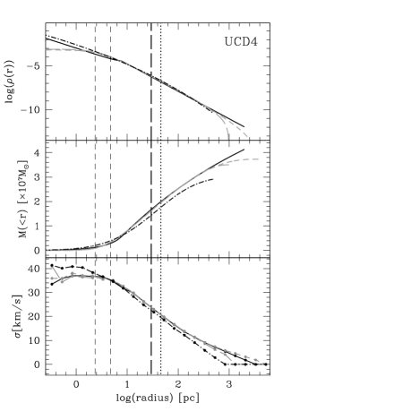
Figure 6: The model output of four different light profile representations of UCD4 is shown; the line types are: black solid - Nuker law, black dot-dashed - Sersic law, grey long dashed - King profile, grey short dashed - generalized King profile. The upper panel shows the 3-dimensional density distribution, the middle panel the cumulative mass distribution, and the lower panel the projected velocity dispersion profile of the $z$-component of the 3-dimensional velocity. The vertical short dashed lines indicate the radii of 0.5 (left) and 1 pixel. The dotted line is half the slit width, and the bold dashed line shows the projected half-light radius of UCD4.

Figure 7: The model output of two different light profile representations of UCD3 is shown; the line types are: solid - 2-component King+Sersic profile, dashed - Nuker law. The upper panel shows the 3-dimensional density distribution, the middle panel the cumulative mass distribution, and the lower panel the projected velocity dispersion profile of the $z$-component of the 3-dimensional velocity. The vertical short dashed lines indicate the radii of 0.5 (left) and 1 pixel. The dotted line is half the slit width, and the bold dashed line shows the projected half-light radius of UCD3.

In case of the Nuker and Sersic functions, the models were truncated at large radii to avoid the unphysical infinite extensions of UCD light profiles. The truncation radius of the Nuker model was fixed at 2 kpc. Depending on the steepness of the outer power law the total mass estimate can depend critically on the exact value of the truncation radius. See, for example the rising cumulative mass of UCD4 in Fig. 6 (middle panel). The truncation radius of the Sersic model was set to 20 times the effective radius, thus ranging between some hundred parsecs and a few kiloparsecs for the UCDs in our sample. In some cases, the adopted truncation radius might be too short leading to lower values of the total mass as compared to other models (see Fig. 6, middle panel).

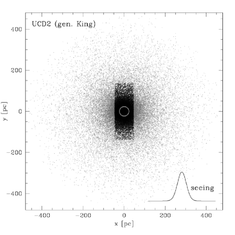
Figure 8: The $x$-$y$-plane of the modelled generalized King representation of UCD2 is shown. Grey dots are all 100.000 test particles. Black dots are those ‘stars’ whose centres fall into the analysed slit area. The grey circle indicates the projected half-light radius of UCD2. The Gaussian in the lower right corner corresponds to the convolution kernel used to estimate the fraction of light that falls into the slit region for each ‘star’.

The true tidal radii of the UCDs depend on their distances to the cluster center $R_{G}$ and the mass $m_{c}$ of the cluster (UCD). It can be estimated by the formula: $r_{t}=(Gm_{c}/2v_{\rm circ}^{2})^{1/3}R_{G}^{2/3}$, where $v_{\rm circ}$ is the circular velocity of the cluster potential and $G$ the gravitational constant. For the Fornax cluster, the circular velocity is about 420 km s^-1 (e.g. Richtler et al. rich04 (2004)), and the projected distances of the UCDs are between 30 and 180 kpc. The resulting lower limits (because of projected distances) of the tidal radii range between 1 and 2 kpc, agreeing with the adopted truncation radii.

After the creation of the UCD model the velocity dispersion as seen by an observer is calculated. To achieve this, the following steps are performed:

1. All test particles are convolved with a Gaussian whose full-width at half-maximum (FWHM) corresponds to the observed seeing.

2. The fraction of the ‘light’ (Gaussian) that falls into the slit at the projected distance of the observed object (the size of the slit in arcsec and the distance to the object in Mpc are input parameters) is calculated.

3. These fractions are used as weighting factors for the velocities. All weighted velocities that fall into the slit region are then used to calculate the ‘mimicked’ observed velocity dispersion $\sigma_{\rm mod}$.

Of course, the total ‘true’ mass of the modelled object, $M_{\rm true}$, that corresponds to the observed velocity dispersion, $\sigma_{\rm obs}$ is not known a priori. One has to start with a first guess of the total mass, $M_{\rm guess}$, from which the ‘true’ mass can be calculated as $M_{\rm true}=M_{\rm guess}\cdot(\sigma_{\rm obs}/\sigma_{\rm mod})^{2}$.

As an example, in Fig. 8 the $x$-$y$-plane of the modelled generalized King representation of UCD2 is shown. The black dots indicate ‘stars’ whose centres fall into the analysed slit area ($1\times 3$ arcsec); the Gaussian represents the point spread function profile of the ‘stars’ caused by the seeing conditions during the observations (see Table 1). In Fig. 9 the velocity histograms of all particles for two model representations of UCD4 are shown. The particles in the histograms are the ones in the slit area and the luminosity weighted number counts of those particles whose ‘light’ falls into the slit area. One can see that the seeing hardly changes the velocity dispersion for stars within the slit region. This is because most of the objects’ light is contained in the analysis area (e.g. the half-light radii of UCDs are smaller than the slit width). Though, the total as well as central velocity dispersion (see also Table 6) can differ significantly from the observed one due to the extended light profiles and central concentration of the models, respectively.

4.2 Dynamical masses

The results of the modelled cluster masses and velocity dispersions for King, generalized King, Sersic, Nuker and King+Sersic functions are presented in Table 6, together with the surface brightness profile model parameters which were taken from Table 9 in Evstigneeva et al. (evst06 (2006)).

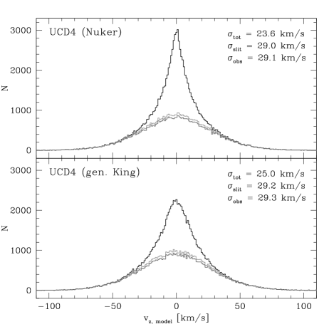
Figure 9: Velocity histograms of the $z$-component velocities for the Nuker (top panel) and generalized King (lower panel) models of UCD4. The bin width is 1 km s^-1. Black solid lines indicate the velocity distributions of all test particles, the light grey lines those of the ‘stars’ with centres in the slit area, and the grey lines the luminosity weighted number counts of those ‘stars’ whose ‘light’ falls into the slit area. The corresponding velocity dispersions are given in the plots.

The errors of the modelled masses were estimated from the uncertainty in the observed velocity dispersion, $\Delta\sigma$ and from typical uncertainties of model parameters for surface brightness profiles (see Evstigneeva et al. evst06 (2006)). On the one hand, maximum and minimum model masses were estimated using the minimum and maximum observed velocity dispersion $(\sigma_{\rm obs}+\Delta\sigma)$ and $(\sigma_{\rm obs}-\Delta\sigma)$, respectively. The average of the differences $(M_{\rm max}-M_{\rm true})$ and $(M_{\rm true}-M_{\rm min})$ defines the first mass error. On the other hand, models were created that simulate $\sigma_{\rm obs}$ from the profile parameters plus/minus their uncertainties. The maximum and minimum mass deviations from $M_{\rm true}$ define the second error. Both errors then were summed to derive the total mass error.

Table 6: Mass modelling results for different light profile representations. The modelled projected half-light radius $r_{h,p}$, central velocity dispersion $\sigma_{0}$, global velocity dispersion $\sigma$, mass and mass-to-light ratio in the $V$-band are given. The adopted surface brightness profile parameters are taken from Evstigneeva et al. (evst06 (2006)). Radii ($R_{b}$, $R_{e}$, $R_{c}$ and $R_{t}$) are in pc; $\mu_{\rm 0,King}$ and $\mu_{e,\rm Sers.}$ are in mag arcsec^-2 in the $V$ band. In the last rows the results for the virial mass estimator are given. The effective radius $R_{\rm eff}$ was taken from Table 10 of Evstigneeva et al. (evst06 (2006)), the global velocity dispersion from the generalized King models and King + Sersic models in two-component fits case. Also the ellipticies ($\epsilon=1-b/a$) from Evstigneeva et al. are shown for reference. The values in bold face were adopted for further analyses.

Model							$r_{h,p}$	$\sigma_{0}$	$\sigma$	$M_{\rm mod}$	$M_{\rm mod}/L_{V}$
							[pc]	[km s-1]	[km s-1]	$\times 10^{7}M_{\odot}$
Nuker:	$R_{b}$	$\alpha$	$\beta$	$\gamma$
UCD1	36.7	0.34	3.03	0.91	…	…	$39.1\pm 3.0$	$51.4\pm 3.0$	$25.2\pm 2.0$	$2.59\pm 0.32$	$4.03\pm 0.53$
UCD2	4.3	0.73	2.38	0.58	…	…	$39.4\pm 3.0$	$33.6\pm 1.0$	$20.4\pm 2.0$	$2.39\pm 0.38$	$3.45\pm 0.59$
UCD3	318.7	1.90	7.04	1.10	…	…	$89.2\pm 8.0$	$33.0\pm 1.8$	$22.7\pm 3.3$	$9.06\pm 2.25$	$3.95\pm 1.00$
UCD4	7.3	20.00	2.13	0.88	…	…	$50.4\pm 4.0$	$36.4\pm 1.2$	$23.6\pm 3.6$	$4.13\pm 1.02$	$5.06\pm 1.31$
Sersic:	$R_{e}$	$n$
UCD1	36.9	9.9	…	…	…	…	$33.1\pm 3.5$	$47.3\pm 4.5$	$26.1\pm 3.0$	$2.59\pm 0.48$	$4.03\pm 0.77$
UCD2	26.6	6.8	…	…	…	…	$25.7\pm 2.5$	$35.5\pm 0.8$	$21.8\pm 2.5$	$1.93\pm 0.39$	$2.79\pm 0.58$
UCD4	24.1	5.5	…	…	…	…	$23.8\pm 2.5$	$40.0\pm 1.1$	$26.3\pm 4.8$	$2.91\pm 0.96$	$3.56\pm 1.22$
King, $\alpha=2$:	$R_{c}$	$R_{t}$	$c$
UCD1	1.8	5761.2	3.51	…	…	…	$49.2\pm 3.5$	$40.7\pm 1.0$	$24.3\pm 4.0$	$4.17\pm 1.04$	$6.49\pm 1.61$
UCD2	2.3	1457.5	2.80	…	…	…	$28.3\pm 1.5$	$31.5\pm 0.8$	$21.2\pm 3.0$	$2.40\pm 0.58$	$3.47\pm 0.86$
UCD4	2.8	987.6	2.55	…	…	…	$26.1\pm 1.3$	$36.4\pm 1.3$	$25.6\pm 5.1$	$3.50\pm 1.22$	$4.29\pm 1.55$
King, var. $\alpha$:	$R_{c}$	$R_{t}$	$c$	$\alpha$
UCD1	1.8	378.0	2.32	0.74	…	…	$22.4\pm 1.0$	41.3$\pm$1.0	27.1$\pm$1.8	3.21$\pm$0.36	4.99$\pm$0.60
UCD2	2.2	487.1	2.35	1.23	…	…	$23.2\pm 1.0$	31.3$\pm$0.6	21.6$\pm$1.8	2.18$\pm$0.31	3.15$\pm$0.49
UCD4	3.0	4501.2	3.18	3.32	…	…	$29.6\pm 2.0$	37.3$\pm$0.6	25.0$\pm$3.4	3.73$\pm$0.86	4.57$\pm$1.11
King+Sersic:	$R_{c}$	$R_{t}$	$\mu_{\rm 0,King}$	$R_{e}$	$n$	$\mu_{e,\rm Sers.}$
UCD3	3.6	119.2	15.74	106.6	1.34	21.13	$89.9\pm 6.0$	29.3$\pm$1.2	22.8$\pm$3.1	9.45$\pm$2.20	4.13$\pm$0.98
UCD5	4.0	30.7	15.13	134.5	6.9	24.04	$30.0\pm 2.5$	28.7$\pm$0.8	18.7$\pm$3.2	1.80$\pm$0.50	3.37$\pm$0.85
FCC303	1.2	2403.9	13.32	696.3	0.6	22.81	$668.3\pm 12.$	37.8$\pm$3.5	16.5$\pm$3.9	33.15$\pm$9.53	2.47$\pm$0.72
Virial mass estimator:						$\epsilon$		$R_{\rm eff}$	$\sigma$	$M_{\rm vir}$	$M_{\rm vir}/L_{V}$
UCD1	…	…	…	…	…	0.18	…	22.4	$27.1\pm 1.8$	$3.73\pm 0.52$	$5.70\pm 0.84$
UCD2	…	…	…	…	…	0.01	…	23.1	$21.6\pm 1.8$	$2.44\pm 0.42$	$3.47\pm 0.62$
UCD3	…	…	…	…	…	0.03	…	92.2	$22.8\pm 3.1$	$10.87\pm 3.04$	$4.66\pm 1.32$
UCD4	…	…	…	…	…	0.05	…	29.5	$25.0\pm 3.4$	$4.18\pm 1.17$	$5.03\pm 1.43$
UCD5	…	…	…	…	…	0.24	…	31.2	$18.7\pm 3.2$	$2.47\pm 0.87$	$4.54\pm 1.61$
FCC303	…	…	…	…	…	0.03	…	660.0	$16.5\pm 3.9$	$40.74\pm 19.3$	$2.98\pm 1.42$

The mass-to-light ratio errors were propagated from the mass errors and the uncertainty in the luminosity (assumed to be 0.05 mag in the absolute magnitude). The luminosities were derived from the apparent, extinction corrected $V$ magnitude as given in Table 1, a distance modulus to Fornax of $(m-M)_{V}=31.39$ mag (Freedman et al. freed01 (2001)) and a solar absolute $V$ magnitude of $M_{V,\odot}=4.85$ mag.

The error of the central velocity dispersion was estimated from the observational error plus the scatter of modelled velocity dispersions in annuli of 0.5 parsec within the central 5 pc for each object. The error of the global velocity dispersion is the sum of the observational error and the uncertainties as propagated from the mass error of the profile parameters.

The masses and $M/L$ values of the different models in general agree with each other within the errors. In Fig. 10, the luminosity versus mass plane is shown for all model results and the virial mass estimate (see below). The mass-to-light ratios of most UCDs scatter around $M/L_{V}=4$. On average, the masses of the Sersic profile are slightly lower than those derived from the other profiles, mainly caused by the adopted truncation radius (see discussion above). The masses of the Nuker profile are sensible to the slope of the outer power law and the adopted truncation radius. The shallow outer slope of UCD4 causes a high mass estimate, whereas the rather steep outer slope of UCD1 results in a low mass estimate as compared to the other models. Besides the uncertainties in the truncation radius, Nuker and Sersic mass estimates suffer from the uncertainties in the central parts of the profile. The cuspy nature of the density profile depends on the light distribution within the central 2-4 pixels, an area for which it is difficult to make a model independent of the assumed fitting function (see Fig. 3 in Evstigneeva et al. evst06 (2006)). Most sensitively, the central velocity dispersion $\sigma_{0}$ depends on the model shape within the innermost pixels. The derived $\sigma_{0}$ values for Nuker or Sersic models are 3-10 km s^-1 higher than those for the King models. This has to be taken into account when using central velocity dispersions in fundamental plane plots.

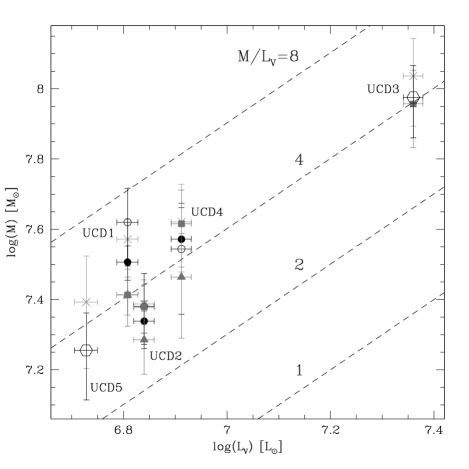
Figure 10: Luminosity vs. mass plot for five Fornax UCDs (the data for UCD1 were taken from Drinkwater et al. (drin03a (2003)). The symbols indicate the following models: grey open circles - King, filled circles - generalized King, grey triangles - Sersic; grey squares - Nuker, open hexagons - King+Sersic, and crosses - virial mass estimator. Lines of constant mass-to-light ratio are shown as indicated.

The most stable results for one-component profile fits are those of the generalized King model because they do not suffer from the uncertain profile shape in the inner pixels (like Nuker and Sersic) and fit the outer regions much better than the ‘normal’ King models. Concerning two-component profiles, King core+Sersic halo models are the most reliable. Therefore, the fit values of these models were adopted for further analyses (see numbers in bold face in Table 6).

The results of our dynamical modelling were also compared with the virial mass estimator by Spitzer (spitz87 (1987)), $M_{\rm vir}\approx 9.75(R_{\rm eff}\sigma^{2})/G$, where $\sigma$ is the global projected velocity dispersion and $R_{\rm eff}$ the half-light radius. This method also assumes a constant $M/L$ ratio as function of radius and an isotropic velocity distribution. The results are shown in Table 6. The errors in the virial mass estimates were propagated from the errors in $R_{\rm eff}$ and $\sigma$. The virial and modelled masses agree within the errors.

4.3 Comparison with masses from stellar population models

In turn the masses and mass-to-light ratios as derived from dynamical modelling are compared with the $M/L$ values expected from stellar population models in order to see whether UCDs can be explained by pure stellar systems or whether they would need dark matter within the central 1-3 half-mass radii to account for missing mass.

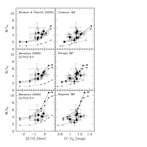
Figure 11: The dynamical $M/L_{V}$ ratios of Fornax UCDs (filled circles) and the nucleus of FCC303 (filled triangle) are compared to expected $M/L_{V}$ values from stellar population models. Also shown are data for Virgo UCDs (open squares from Evstigneeva et al. (evst06 (2006)). In the left panels $M/L_{V}$ is plotted versus metallicity [Z/H], in the right panels versus the colour $(V-I)_{0}$. The references to the models and the adopted IMF are indicated in the panels. The three lines in each plot represent ages of 15, 13 and 5 Gyr from top to botton, respectively. For the Fornax UCDs an $\alpha$ abundance of [$\alpha$/Fe]$=0.3$ was adopted to derive their [Z/H] values. Note, however, that their $\alpha$ abundance might be different (solar) if they possess a significant contribution of intermediate age stellar populations.

There are stellar population models available from various groups. Here we present the comparison with Bruzual & Charlot (bruz03 (2003)) and Maraston (mara05 (2005)) models. Mass-to-light ratios are given for single stellar populations (SSPs) of various ages and metallicities. The metallicity in the Maraston models is a total metallicity [Z/H] including possible [$\alpha$/Fe] overabundances. [Z/H] and the iron abundance [Fe/H] are related as following: [Fe/H] $=$ [Z/H] $-0.94\cdot$[$\alpha$/Fe] (Thomas et al. thoma03 (2003)). [Z/H] is in agreement with the Zinn & West (zinn84 (1984)) scale.

In Fig. 11, the dynamical masses of Fornax UCDs and the nucleus of FCC 303 are compared to stellar population models in the [Z/H] versus $M/L_{V}$ and $(V-I)$ versus $M/L_{V}$ plane. For comparison we also include data for seven of the brightest Virgo UCDs (Evstigneeva et al. evst06 (2006)). Three sets of models with different assumption for the initial mass function (IMF) are presented. The Bruzual & Charlot models with a Chabrier IMF, and the Maraston models with a Kroupa as well as a Salpeter IMF. These IMFs were chosen to illustrate the wide range of predictions from various SSP models. The colours of the Virgo UCDs were taken from Evstigneeva et al. (evst06 (2006)). The ages, metallicities and $\alpha$ abundances were estimated from diagnostic plots of line indices in Evstigneeva et al. (Figs. 11 & 12). Most Virgo UCDs are old (8 to 15 Gyr), and most of them show super-solar [$\alpha$/Fe] values around 0.3 dex. The iron abundances and colours of the Fornax UCDs were taken from Mieske et al. (mies06 (2006)). No age and $\alpha$-abundance estimates are published for them. The relatively high Balmer line H$\beta$ indices of UCD3 and UCD4 (see Table 1 in Mieske et al. mies06 (2006)) might point to a contribution of young to intermediate age stellar populations within these UCDs. Note that this statement has to be taken with caution since no proper calibration of the line indices was performed in Mieske at al.’s paper.

Fig. 11 shows that the dynamical masses of all UCDs and the nucleus can be reconciled with stellar population models if taking the ‘right’ set of models. The Bruzual & Charlot models with a Chabrier IMF tend to predict $M/L_{V}$ values that are lower than the measured ones. Taking these models at face value one might conclude that most UCDs need some amount of dark matter to explain their higher $M/L_{V}$ values. When taking Maraston models with a Salpeter IMF, however, even the extreme case of Strom417 (a low mass UCD or massive GC) with a dynamical $M/L_{V}$ value around 6 (Evstigneeva et al. evst06 (2006), Haşegan et al. hase05 (2005)) can be explained by an old stellar population. If these models are correct for all UCDs, many of them are best fitted by intermediate age (5-8 Gyr) stellar populations. In the Fornax cluster, UCD2, UCD3 and the nucleus of FCC303 would be candidates for young ages, whereas UCD1, UCD4 and UCD5 still are compatible with old stellar populations. In the Virgo cluster, VUCD3, VUCD5 and VUCD6 are possibly younger than the other UCDs. This, however, contradicts the findings by Evstigneeva et al. (evst06 (2006)) who derived old ages for basically all UCDs in Virgo.

It is clear from the discussion above that to decide whether dynamical masses of UCDs are really consistent with a pure stellar population is not straightforward. On the one hand, more accurate ages, metallicities and $\alpha$-abundances are needed to better constrain the right choice of the stellar population models (i.e. to constrain the IMF). On the other hand, there still is the freedom of adding an extended dark matter halo when modelling the UCDs for deriving their masses. In this case, also Bruzual & Charlot models with a Chabrier IMF could be the ‘right’ choice.

The most important result that comes out from our comparison between dynamical and stellar population model masses is that all UCDs and the nucleus of FCC 303 can, in principle, be explained by a pure stellar population. Dark matter is not mandatory for any of the objects within 1-3 half-mass radii. As mentioned before, it can not be ruled out, however, that UCDs are dominated by dark matter at large radii where high signal-to-noise spectra hardly can be obtained due to the very low surface brightness.

5 Summary and Conclusions

In this paper we have presented the spectroscopic analysis of four ultra-compact dwarf galaxies (UCDs) and one nucleus of a dwarf elliptical. These UCDs are among the five brightest in the central region of the Fornax cluster (Hilker et al. hilk99c (1999), Drinkwater et al. drin03a (2003)). The analysis is based on high resolution spectra obtained with the instrument UVES mounted in the VLT at El Paranal, Chile. Velocity dispersions were derived from selected wavelength regions using the direct-fitting method by van der Marel (van der Marel & Franx vdma93 (1993)). To derive the masses of the UCDs a new modelling program has been developed that allows to choose between different representations of the surface brightness profile (i.e. Nuker, Sersic or King laws) and corrects the observed velocity dispersions for observational parameters (i.e. seeing, slit size). The light profile parameters of the UCDs and the nucleus of FCC 303 were obtained from Hubble Space Telescope imaging (see the accompanying paper by Evstigneeva et al. evst06 (2006)). The derived dynamical masses then have been compared to those expected from stellar population models. The main results of our analysis are as follows:

(i) The observed velocity dispersions of the Fornax UCDs range between 22 and 30 km s^-1, slightly smaller than those of Virgo UCDs (Evstigneeva et al. evst06 (2006)) and DGTOs (Haşegan et al. hase05 (2005)). The observed velocity dispersions of the Na doublet regions are systematically higher than those of the other regions, probably reflecting the contribution of stars from different evolutionary stages.

(ii) The generalized King models for the one-component fits and King+Sersic models for the two-component fits were adopted to determine the masses of the UCDs, which range between 1.8 and $9.5\times 10^{7}M_{\odot}$. The corresponding central and global projected velocity dispersions are in the range 29 to 41 and 19 to 27 km s^-1, respectively. The masses as derived from Nuker and Sersic models depend on the adopted truncation radius and the slope of the outer power law (Nuker). Truncation radii that are too small lead to underestimated masses (e.g. Sersic model of UCD4) and flat outer power laws to a steeply increasing cumulative mass profile (e.g. Nuker model of UCD4). The central velocity dispersion mainly depends on the shape of the light profile within the innermost parsecs. If the cuspy behaviour of some UCDs is true, the central velocity dispersion would be up to 10 km s^-1 higher than derived from generalized King models.

(iii) The mass-to-light ratios $M/L_{V}$ of the Fornax UCDs range between 3 and 5. These values are compatible with predictions from stellar population models, especially those from Maraston (mara05 (2005)) assuming a Kroupa or Salpeter IMF. A Salpeter IMF, however, would imply that about half of the Fornax UCDs would be dominated by intermediate age populations of 4 to 8 Gyr. The high Balmer H$\beta$ indices of three UCDs in Fornax is consistent with this interpretation (Mieske et al. mies06 (2006)). Also the $M/L_{V}$ values of all Virgo UCDs can be explained by stellar population models (see Evstigneeva et al. evst06 (2006)). No dark matter component is needed for UCDs whithin 1-3 half-mass radii. One can, however, not rule out that UCDs might be dominated by dark matter in the outer parts.

(iv) The mass-to-light ratio $M/L_{V}$ of the nucleus of FCC 303 is 2.5, entirely compatible with a pure stellar population and similar to those of other dwarf elliptical nuclei (Geha et al. geha02 (2002)).

We conclude that ultra-compact dwarf galaxies most probably are the result of cluster formation processes (i.e. like large globular clusters, assembled star cluster complexes, nuclear star clusters) rather than being genuine cosmological sub-structures themselves (i.e. compact galaxies formed in small, compact dark matter halos).

Massive star clusters (and star cluster complexes) nowadays form in interacting galaxies like the Antennae (e.g. Whitmore et al. whitm99 (1999)). It has been shown that the most massive and compact young massive clusters (YMCs) and star cluster complexes can survive their ‘infant mortality’ (e.g. Fellhauer & Kroupa fell02a (2002), Bastian et al. 2006a ). The most massive surviving YMCs have masses comparable to those of the UCDs presented in this paper (NGC7252:W3, Maraston et al. mara04 (2004); NGC7252:W30, NGC1316:G114, Bastian et al. 2006b ). It is reasonable to assume that similar massive clusters have formed in merger events of the early epochs of galaxy cluster formation. Some of them might have survived the disruption and merging of galaxies during the galaxy cluster formation process as free-floating ‘UCDs’.

But also the threshing of nucleated dwarf galaxies can not be ruled out definitely as formation process of UCDs. Nuclear star clusters as massive as UCDs were able to form either by the merging of globular clusters through tidal friction in early-type dwarf galaxies (e.g. Oh & Lin oh00 (2000), Lotz et al. lotz01 (2001)) or through successive central starbursts in late-type bulge-less spirals. During the dynamical evolution of galaxy clusters many of these low mass nucleated galaxies may be disrupted (e.g. Moore et al. moor99a (1999)). Their debris then is distributed in the intra-cluster medium, building up the extended cD halos of central galaxies (e.g. Hilker et al. hilk99b (1999)). Their globular clusters and nuclei are expected to survive as intra-cluster stellar populations, among them the present-day dark matter-free ‘UCDs’.

In order to differentiate between the formation of UCDs via super-star cluster formation in starbursts and the formation via tidal disruption of nucleated (dwarf) galaxies detailed analysis of the chemical composition and age structure of the stellar population in UCDs might help. A super-solar [$\alpha$/Fe] abundance (as suggested for most of the Virgo UCDs, Evstigneeva et al. evst06 (2006)) would point to a rapid, short-timescale formation process which is typical for old globular clusters. A galaxy nucleus would only show a super-solar [$\alpha$/Fe] value if its star formation was truncated soon after its initial burst or if it would be composed of merged GCs which themselves have super-solar $\alpha$ abundances. However, present-day nuclei of dwarf ellipticals seemed to have formed in a rather continuous way since their $\alpha$-abundances are enriched to solar values (Geha et al. geha03 (2003)). It has to be seen whether the $\alpha$-abundances of the Fornax UCDs are the same as for the Virgo UCDs. Intermediate age populations in UCDs would indicate that some Gyr ago gas still was present in UCDs, constraining the threshing timescale and/or the time of the last major star formation event. Note that there are some hints that Fornax UCDs might be different to Virgo UCDs (e.g. Mieske et al. mies06 (2006)). Maybe also the environment plays a role in their formation processes.

Independent of which scenario is right it is interesting to note that star clusters more massive than about $5\times 10^{6}M_{\odot}$ seem to behave different than less massive ‘ordinary’ GCs. Not only the scaling and fundamental plane relations of massive clusters start to deviate from those of normal GCs (see results and discussions in Kissler-Patig et al. kiss06 (2006) and Evstigneeva et al. evst06 (2006)), but also their stellar populations are getting more complex. Massive clusters do not possess a single stellar population, but are composed of sub-populations if different metallicities and/or ages. The best example is the most massive globular cluster in our Milky Way, $\omega$ Centauri, whose stellar populations revealed a broad metallicity distribution as well as an extended star formation history (e.g. Hilker & Richtler hilk00b (2000), Hilker et al. hilk04a (2004)). Also G1, one of the most massive GCs of M31 is suspected to contain multiple stellar populations (e.g. Meylan et al. meyl01 (2001)). It would be interesting to know whether this is true for all massive clusters, including UCDs.

Although our study has shown that UCDs most probably can be explained by pure stellar populations, more constraints from observations are needed in order to get further insights into their nature. High signal-to-noise spectra for the Fornax UCDs would be useful to derive more accurate chemical abundances and age estimates from appropriate line indices. This should clarify whether they are enhanced in $\alpha$ elements and whether they posses intermediate age populations. Also high resolution spectroscopy (to obtain internal velocity dispersions) of more UCDs and galactic nuclei is needed to fill the parameter space (fundamental plane) in the interface between globular clusters and dwarf galaxies. The most extended UCDs might be targets for spatially resolved high resolution spectroscopy. This would show whether our modelled velocity dispersion profiles are real or whether one would need more sophisticated modelling to comply with possible orbital anisotropies and/or violation of the virial equilibrium through tidal effects. Spatially resolved velocity dispersion profiles also will allow to constrain the shape and mass of extended dark matter halos around UCDs if they existed.

- (1) Bassino, L. P., Muzzio, J. C., & Rabolli, M. 1994, ApJ, 431, 634
- (2) Bastian, N., Emsellem, E., Kissler-Patig, M., & Maraston, C. 2006a, A&A, 445, 471
- (3) Bastian, N., Saglia, R. P., Goudfrooij, P., et al. 2006b, A&A, 448, 881
- (4) Bekki, K., Couch, W. J., Drinkwater, M. J., & Shioya, Y. 2003, MNRAS, 344, 399
- (5) Binney, J., & Tremaine, S. 1987, in: Galactic dynamics, Princeton Univ. Press (Princeton, New Jersey)
- (6) Bruzual, G. A., & Charlot, S. 2003, MNRAS, 344, 1000
- (7) Côté, P., Piatek, S., Ferrarese, L., et al. 2006, ApJS, 165, 57
- (8) De Propris, R., Phillipps, S., Drinkwater, M.J., et al. 2005, ApJ, 623, L105
- (9) Drinkwater, M. J., Gregg, M. D., Couch, W. J., et al. 2004, PASA, 21, 375
- (10) Drinkwater, M. J., Gregg, M. D., Hilker, M., et al. 2003, Nature, 423, 519
- (11) Drinkwater, M. J., Jones, J. B., Gregg, M. D., & Phillipps S. 2000, PASA, 17, 227
- (12) Drinkwater, M. J., Phillipps, S., Gregg, M. D., et al. 1999, ApJ, 511, L97
- (13) Evstigneeva, E. A., Gregg, M. D., Drinkwater, M. D., & Hilker, M. 2006, AJ, submitted
- (14) Fellhauer, M. & Kroupa, P. 2002, MNRAS, 330, 642
- (15) Fellhauer, M. & Kroupa, P. 2006, MNRAS, 367, 1577
- (16) Ferguson, H. C. 1989, AJ, 98, 367
- (17) Freedman, W. L., Madore, B. F., Gibson, B. K., et al. 2001, ApJ, 553, 47
- (18) Geha, M., Guhathakurta, P., & van der Marel, R. P. 2002, AJ, 124, 3073
- (19) Geha, M., Guhathakurta, P., & van der Marel, R. P. 2003, AJ, 126, 1794
- (20) Haşegan, M., Jordán, A., Côté, P., et al. 2005, ApJ, 627, 203
- (21) Hilker, M., Infante, L., & Richtler, T. 1999, A&AS, 138, 55
- (22) Hilker, M., Infante, L., Vieira, G., Kissler-Patig, M., & Richtler, T. 1999, A&AS, 134, 75
- (23) Hilker, M., Kayser, A., Richtler, T., & Willemsen, P. 2004, A&A, 422, L9
- (24) Hilker, M., & Richtler, T. 2000, A&A, 362, 895
- (25) Jones, J. B., Drinkwater, M. J., Jurek, R., et al. 2006, AJ, 131, 312
- (26) Jordán, A., Côté, P., Blakeslee, J. P., et al. 2005, ApJ, 634, 1002
- (27) Karick, A. M., Drinkwater, M. J., & Gregg, M. D. 2003, MNRAS, 344, 188
- (28) Kissler-Patig, M., Jordán, A., & Bastian, N. 2006, A&A, 448, 1031
- (29) Kroupa P. 1998, MNRAS, 300, 200
- (30) Lotz, J. M., Miller, B. W., & Ferguson, H. C. 2004, ApJ, 613, 262
- (31) Lotz, J. M., Telford, R., Ferguson, H. C., et al. 2001, ApJ, 552, 572
- (32) Maraston, C. 2005, MNRAS, 362, 799
- (33) Maraston, C., Bastian, N., Saglia, R. P., et al. 2004, A&A, 416, 467
- (34) Martini, P., & Ho, L. C. 2004, ApJ, 610, 233
- (35) Meylan, G., Sarajedini, A., Jablonka, P., et al. 2001, AJ, 122, 830
- (36) Mieske, S., Hilker, M., & Infante, L. 2002, A&A, 383, 823
- (37) Mieske, S., Hilker, M., & Infante, L. 2004, A&A, 418, 445
- (38) Mieske, S., Hilker, M., Infante, L., & Jordán, A. 2006, AJ, 131, 2442
- (39) Moore, B., Lake, G., Quinn, T., & Stadel, J. 1999, MNRAS, 304, 465
- (40) Oh, K. S., & Lin, D. N. C. 2000, ApJ, 543, 620
- (41) Phillipps, S., Drinkwater, M. J., Gregg, M. D., & Jones, J. B. 2001, ApJ, 560, 201
- (42) Richtler, T. 2006, Bull. Astr. Soc. India, 34, 83
- (43) Richtler, T., Dirsch, B., Gebhardt, K., et al. 2004, AJ, 127, 2094
- (44) Richtler, T., Dirsch, B., Larsen, S., Hilker, M., & Infante, L. 2005, A&A, 439, 533
- (45) Schlegel, D. A., Finkbeiner, D. P., & Davis, M. 1998, ApJ, 500, 525
- (46) Spitzer, L. 1987, in: Dynamical Evolution of Globular Clusters (Princeton: Princeton Univ. Press)
- (47) Thomas, D., Maraston, C., & Bender, R. 2003, MNRAS, 339, 897
- (48) Tonry, J., & Davis, M. 1979, AJ, 84, 1511
- (49) van der Marel, R. P., & Franx, M. 1993, ApJ, 407, 525
- (50) van de Ven, G., van den Bosch, R. C. E., Verolme, E. K., & de Zeeuw, P. T. 2006, A&A 445, 513
- (51) van Dokkum, P. G. 2001, PASP, 113, 1420
- (52) Walcher, C. J., van der Marel, R. P., McLaughlin, D., et al. 2005, ApJ, 618, 237
- (53) Whitmore, B. C., Zhang, Q., Leitherer, C., et al. 1999, AJ, 118, 1551
- (54) Zinn, R., & West, M. J. 1984, ApJS, 55, 45