The origin of the reversed granulation in the solar photosphere

Abstract

We study the structure and reveal the physical nature of the reversed granulation pattern in the solar photosphere by means of 3-dimensional radiative hydrodynamics simulations. We used the MURaM code to obtain a realistic model of the near-surface layers of the convection zone and the photosphere. The pattern of horizontal temperature fluctuations at the base of the photosphere consists of relatively hot granular cells bounded by the cooler intergranular downflow network. With increasing height in the photosphere, the amplitude of the temperature fluctuations diminishes. At a height of $z=130-140$ km in the photosphere, the pattern of horizontal temperature fluctuations reverses so that granular regions become relatively cool compared to the intergranular network. Detailed analysis of the trajectories of fluid elements through the photosphere reveal that the motion of the fluid is non-adiabatic, owing to strong radiative cooling when approaching the surface of optical depth unity followed by reheating by the radiation field from below. The temperature structure of the photosphere results from the competition between expansion of rising fluid elements and radiative heating. The former acts to lower the temperature of the fluid whereas the latter acts to increase it towards the radiative equilibrium temperature with a net entropy gain. After the fluid overturns and descends towards the convection zone, radiative energy loss again decreases the entropy of the fluid. Radiative heating and cooling of fluid elements that penetrate into the photosphere and overturn do not occur in equal amounts. The imbalance in the cumulative heating and cooling of these fluid elements is responsible for the reversal of temperature fluctuations with respect to height in the photosphere.

1 Introduction

In the quiet Sun, the most prominent photospheric feature is the surface granulation pattern. Observations in white light show bright granules with a typical size of $1$ Mm, embedded in a network of dark intergranular downflow lanes and vertices. The granulation pattern is non-stationary: studies of time-sequences of the granulation pattern in the quiet Sun show that individual features evolve with an average lifetime of about $5$ minutes (e.g. Title et al., 1989).

While intensity images in the visible continuum taken near disk-center show bright granules and comparatively dark intergranular boundaries, observations taken in the wings of the Ca II H & K lines exhibit a similar pattern, but with reversed intensity contrast (Evans & Catalano, 1972; Suemoto, Hiei, & Nakagomi, 1987, 1990). This effect, known as the reversed granulation, has also been detected in intensity measurements of photospheric spectral lines (Espagnet et al., 1995; Balthasar et al., 1990; Kucera et al., 1995; Rodríguez Hidalgo et al., 1999; Janssen & Cauzzi, 2006). These observations suggest that the reversal of the intensity contrast occurs already at a height of about $150$ km above the mean geometric level where $\tau_{\rm 500}=1$.

Recently, Rutten, de Wijn, & Sütterlin (2004) acquired simultaneous, speckle-reconstructed images of quiet-Sun granulation in the G-band and the Ca II H line. On the basis of cross-correlations between time sequences of intensity images in these two spectral ranges they found that the anticorrelation between the two patterns is highest if the Ca II H intensity maps are time-delayed by $2-3$ minutes with respect to the G-band intensity maps. By computing anticorrelation coefficients between (1) intensity images in the continuum and in the  Fe I 7090  Å line and (2) intensity images in the continuum and in the wing of the Ca II 8542 Å line, Janssen & Cauzzi (2006) also found that the strongest anticorrelation occurs for a time delay of $\sim 2$ min. Leenaarts & Wedemeyer-Böhm (2005) extended the work of Rutten, de Wijn, & Sütterlin (2004) by calculating synthetic intensity images in the blue continuum and in the Ca II H wing (in the LTE approximation) from a 3-dimensional radiative hydrodynamic simulation. From the unsmoothed synthetic intensity images, they found that the anticorrelation between the continuum images and the Ca II H wing images does not vary significantly between a time delay of $0$ and $2$ minutes. The anticorrelation decreased for longer time delays. When the images were smoothed to $1.5$ arcsec resolution, a time-delay of $2-3$ minutes yielded a significantly higher value of the anticorrelation compared to zero time delay.  Rutten, de Wijn, & Sütterlin (2004) speculated that magnetic fields play no major role in the formation of the reversed granulation. The results of Leenaarts & Wedemeyer-Böhm (2005) is evidence supporting this view.

Numerical simulations have firmly established the solar granulation as a radiative-convective phenomenon (Nordlund, 1984, 1985; Steffen et al., 1989; Stein & Nordlund, 1998). Granules are upwellings of hot, high-entropy material originating from the convection zone and overshooting into the stably stratified photosphere. Radiative losses make the overshooting material relatively cold and dense. Its overturning motion supplies the network of intergranular downflows. Simulations have also revealed that the pattern of horizontal temperature fluctuations in the middle/upper photosphere is inverted compared to the corresponding pattern at the base of the photosphere. Whereas at the base of the photosphere, the granules are relatively hot compared to the intergranular network, the former are relatively cooler for $\tau_{\rm 500}\lesssim 0.3$. It is well known that this reversal in the temperature fluctuations in the photosphere is responsible for the reversal in the observed intensity pattern (Nordlund, 1984; Suemoto, Hiei, & Nakagomi, 1987; Leenaarts & Wedemeyer-Böhm, 2005).

What is less clear is the physical mechanism which leads to the reversal of the temperature fluctuations with height. It is sometimes incorrectly assumed that fluid travelling in the optically thin layers of the photosphere does so adiabatically. As pointed out by Nordlund (1984), this cannot be true because material with an original temperature of $5900$ K penetrating and expanding adiabatically in the photosphere would reach a temperature of $1800$ K after traversing only three pressure scale heights. Such low temperatures are not detected in the photosphere. Stein & Nordlund (1998) indeed find that fluid rising in the photosphere is typically reheated by the radiation field. This leads one to conclude that non-adiabatic effects, such as radiative energy exchange, must play a crucial role in the formation of the reversed temperature fluctuations.

The aim of the present paper is to investigate the physical origin of the reversal of temperature fluctuations. As we shall see in the following sections, radiative energy exchange is indeed key to the temperature fluctuation reversal. By following in detail the time histories of fluid elements penetrating into the photosphere, we identify how radiative heating and cooling, in tandem with the horizontal pressure fluctuations, causes the reversed granulation. The paper is structured as follows. In § 2, we describe the set of governing equations, the numerical methods used and the simulation setup. In § 3, we discuss results from the numerical simulation, including the mean stratification of the 3D model (§ 3.1), the temperature structure in the photosphere (§ 3.2) and reveal the physical origin of the reversed granulation (§ 3.3). Finally, in § 4, we discuss how the present work dispels previous misconceptions and improves our understanding of the phenomenon.

2 Simulation setup

2.1 Governing equations

For a realistic treatment of the dynamics and energetics in the near-surface layers of the non-magnetic solar atmosphere, it is important to consider the effects of compressibility, energy exchange via radiative transfer and partial ionization (Stein & Nordlund, 1998; Rast & Toomre, 1993; Rast et al., 1993; Vögler, 2003). The hydrodynamics equations, the radiative transfer equation (RTE) and the equation of state (EOS) including the effects of partial ionization constitute the system of governing equations for our model. Since we are confining our attention to the near-surface layers of the convection zone and the photosphere, the approximation of local thermodynamic equilibrium (LTE) suffices for the treatment of the radiative transfer. The hydrodynamics equations include the continuity equation, the momentum equation and the energy equation, viz.

$$\frac{\partial\varrho}{\partial t} + \nabla\cdot(\varrho\mathbf{v})=0,$$ (1)

$$\frac{\partial\varrho\mathbf{v}}{\partial t} + \nabla\cdot\left(\varrho\mathbf{v}\otimes\mathbf{v}\right)=-\nabla p+\varrho\mathbf{g}+\nabla\cdot\underline{\underline{\tau}},$$ (2)

$$\frac{\partial\varrho\varepsilon}{\partial t} + \nabla\cdot\left(\varrho\mathbf{v}\left[\varepsilon+\frac{p}{\varrho}+\frac{1}{2}|\mathbf{v}|^{2}\right]\right)=$$ (3)

$$\nabla\cdot(\mathbf{v}\cdot\underline{\underline{\tau}})+\nabla\cdot(K\nabla T)+\varrho(\mathbf{g}\cdot\mathbf{v})+Q_{\rm rad},$$

where $\mathbf{v}$ is the fluid velocity, $\varrho$ the mass density and $\varepsilon$ the internal energy density per unit mass. The operator $\otimes$ denotes the tensor product. In the near-surface layers of the Sun, the gravitational acceleration is almost constant and we take $\mathbf{g}=-2.74\times 10^{4}\hat{z}$ cm s^-2.

The hydrodynamics equations (1)-(3) must be supplemented by the appropriate constitutive relations describing the material properties of the gas. These include the equation of state (EOS), functions specifying the viscous stress tensor $\underline{\underline{\tau}}$ and thermal conductivity $K$, as well as functions specifying the radiative properties of the gas (e.g. source function $S_{\nu}$, opacity $\kappa_{\nu}$ etc.). The frequency-integrated radiative heating term appearing on the r.h.s. of Eq. (3) is given by

$$Q_{\rm rad}=\int 4\pi\kappa_{\nu}\varrho(J_{\nu}-\bar{S}_{\nu}){\rm d}\nu,$$ (4)

where $J_{\nu}$ is the angle-averaged specific intensity and $\bar{S}_{\nu}$ the angular-averaged source function.

2.2 Numerical method

For our radiative hydrodynamics simulations, we have used the MPS/University of Chicago Radiative MHD (MURaM) code (Vögler, Shelyag, Schüssler, Cattaneo, Emonet, & Linde, 2005). In the absence of magnetic fields, the equations solved by MURaM reduce to the equations given in the preceding section.

In the following, we briefly describe the numerical methods implemented in MURaM. For further details, we refer the reader to Vögler (2003) and Vögler et al. (2005). MURaM integrates the discretized equations (1)-(3) on a 3-dimensional cartesian grid, with constant grid-spacing in each cartesian direction. The spatial discretization of the equations is based on a fourth-order centered-difference scheme on a five-point stencil. Time-stepping is carried out using an explicit fourth-order Runge-Kutta scheme, with the maximum size of the time step determined by a modified CFL-criterion.

In order to prevent the nonlinear cascade of energy towards the grid scale, artificial diffusivities are implemented to stabilize the simulations. A combination of hyper- and shock-resolving diffusivities are used (Caunt & Korpi, 2001). Hyperdiffusivities are implemented in such a way, that the diffusion terms associated with them are comparable in magnitude to the inertial terms only at length scales close to the grid-spacing. For the thermal and viscous coefficients $K$ and $\nu$, the hyperdiffusivities are defined using the scheme described in Vögler et al. (2005).

The RTE is solved with the short-characteristics method on a 3D cartesian grid, with the grid centers of this radiative grid defined by the cell corners of the grid used for discretizing the hydrodynamics equations (1)-(3). For each point on this radiative grid, the RTE is solved over $24$ ray directions ($3$ per octant). The first moment of $I_{\nu}$ over these rays provides the radiative flux density $\mathbf{F}_{\nu}$, which in turn allows $Q_{\rm rad}$ to be calculated.

MURaM can treat the radiative transfer in the grey or non-grey case (see Vögler, 2004, and references therein). For this study, we have carried out two simulations, namely a grey run and a non-grey run. The results presented in the rest of this paper correspond to the non-grey case. The main difference between the results of the two cases it that the non-grey case yields smaller temperature fluctuations in the photosphere than the grey case. This difference arises because the grey case underestimates the smoothing effects of radiative transfer in the optically thin layers of the photosphere in comparison with the non-grey case (Vögler, 2004). Our explanation for the reversed granulation phenomenon (see § 3.2), however, applies to both cases.

The EOS relations $T=T(\varepsilon,\varrho)$ and $p=p(\varepsilon,\varrho)$ are used by MURaM in the form of look-up tables. The look-up tables were evaluated by solving the Saha-Boltzmann equations. The first ionization of the $11$ most abundant elements was considered. For a detailed account of how the tables were evaluated, we refer the reader to Appendix A of Vögler et al. (2005).

2.3 Simulation setup

In order to obtain a thermally relaxed 3D model of the upper convection zone and the photosphere, we have chosen the following setup. The horizontal size of the simulation domain is $24$ Mm $\times 12$ Mm, with each direction spanned by $480$ and $240$ grid cells, respectively. The height of the domain is $2.3$ Mm, and is spanned by $144$ grid cells. The grid-spacing in the horizontal and vertical directions is $50$ and $16$ km, respectively. Periodic boundary conditions are assumed for the vertical side boundaries. The bottom boundary is open and allows mass to flow smoothly into and out of the domain (see Vögler et al., 2005).

For the initial condition, we took the 1D height profiles of $\varrho$ and $\epsilon$ from the mixing length model of Spruit (1974) and introduced a plane-parallel stratification into the simulation domain. To break the symmetry, we imposed pressure perturbations on the order of a few percent. We then ran the simulation until we obtained a thermally relaxed, statistically stationary state.

3 Simulation results

3.1 Mean stratification

The horizontally averaged profiles of pressure and temperature as functions of height are shown in Fig. 1, respectively, as solid and dashed curves. The geometrical height $z=0$ corresponds to the geometrical level where the continuum optical depth at $500$ nm is, on average, unity. The height dependence of the mean profiles are in general agreement with the simulation results of Stein & Nordlund (1998).

Figure 2 shows the logarithmic temperature gradients determined from the mean profiles:

$$\nabla := \frac{{\rm d}\ln{T}}{{\rm d}\ln{p}},{\rm~{}and}$$ (5)

$$\nabla_{\rm ad} := \left(\frac{\partial\ln{T}}{\partial\ln{p}}\right)_{s}.$$ (6)

$\nabla$ (dotted curve) is the actual average temperature gradient in the simulation and $\nabla_{\rm ad}$ (solid black curve) is the adiabatic temperature gradient. $\nabla_{\rm ad}$ describes the variation of temperature of a fluid element undergoing adiabatic expansion or compression.

Figure 1: Horizontally averaged pressure (solid) and temperature (dashed) as functions of height $z$.

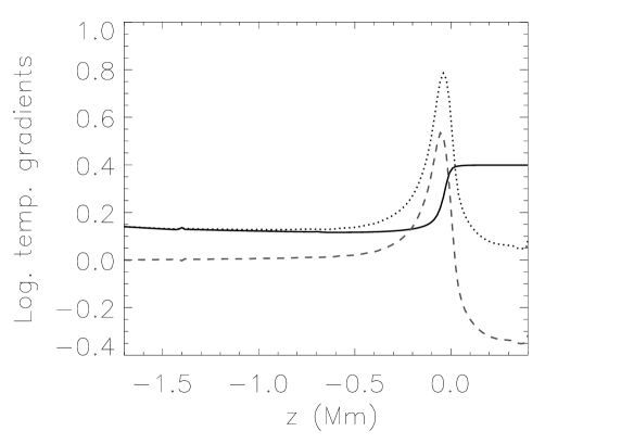
Figure 2: Logarithmic temperature gradients $\nabla$ (dotted curve), $\nabla_{\rm ad}$ (solid black) and the superadiabaticity $\delta=\nabla-\nabla_{\rm ad}$ (dashed curve).

The stability of the stratification to convective motion is affected by changes in the ionization state. The superadiabaticity of the stratification is defined as $\delta:=\nabla-\nabla_{\rm ad}$ and is plotted as a dashed curve in Fig. 2. In the photosphere, the chemical species are almost completely monatomic. For such a gas, $\gamma=5/3$ and hence, $\nabla_{\rm ad}=1-1/\gamma=0.4$. With increasing depth into the convection zone, the ionization fraction of hydrogen (and traces of other species) increases. This has the effect of decreasing the adiabatic temperature gradient, so that $\nabla_{\rm ad}<0.4$ while $\delta$ remains positive. In other words, changes in the ionization state of the gas reduces $\nabla_{\rm ad}$ and thus enhances buoyancy driving.

3.2 The reversal of temperature fluctuations in the middle photosphere

Figure 3: Temperature fluctuations ($\Delta T/\bar{T}$, upper row) and vertical velocity (lower row) at two surfaces of constant optical depth. The left column shows the patterns at $\tau_{\rm 500}=1$, the right $\tau_{\rm 500}=0.1$. The reversed granulation corresponds to a reversal of the temperature fluctuations while the velocity pattern remains qualitatively unchanged.

In this section, we study the reversed granulation in our 3D model. For lines that form under approximate LTE conditions, such as some Fe I lines and the wings of the Ca II H & K lines, fluctuations in line intensity are a proxy for diagnosing temperature fluctuations. The intensity image therefore maps the temperature distribution in the layer of the atmosphere in which the corresponding part of the line is formed. An inspection of the temperature fluctuations at different heights of the atmosphere allows one to determine the height at which the temperature fluctuations start to reverse.

The upper row of Fig. 3 shows the relative temperature fluctuations ($\Delta T/\bar{T}$) at the surfaces $\tau_{\rm 500}=1$ (left column) and $\tau_{\rm 500}=0.1$ (right column). The lower row gives the vertical velocity at the same surfaces. On average, the $\tau_{\rm 500}=0.1$ surface is elevated above the $\tau_{\rm 500}=1$ surface by $160$ km. At $\tau_{\rm 500}=1$, one finds the normal granulation pattern: the granules are hotter than the intergranular lanes. At $\tau_{\rm 500}=0.1$, the reversed granulation is already clearly discernible: the lanes are regions of temperature excess. When we inspect the velocity structure, we find that the pattern at $\tau_{\rm 500}=0.1$ is very similar to that at $\tau_{\rm 500}=1$, albeit with smaller flow speeds. The upflows in the higher layers result from the overshooting of upwelling gas from the convection zone. Thus, the reversal of the pattern of temperature (and intensity) fluctuations is not accompanied by a reversal in the velocity pattern (e.g. see Ruiz Cobo et al., 1996).

In order to determine the geometrical height at which the reversed granulation begins, we consider the vertical velocity and temperature as functions of $z$ for vertical lines of sight (l.o.s.). Distinguishing the l.o.s. profiles according to the sign of the vertical velocity at $\tau_{\rm 500}=1$, we separately determine averages for profiles of the temperature fluctuations in granules and in the intergranular downflow network, respectively. The fluctuations are evaluated relative to the overall average temperature profile. These two quantities are plotted as functions of $z$ in Fig. 4. Diamonds indicate the mean temperature fluctuation in the granules whereas crosses indicate the mean temperature fluctuation in the intergranular lanes. These two are not simply the negative of each other because the cells have a larger area fraction than the boundaries. In the convection zone and in the lower photosphere, upflowing material in the granules are relatively hot compared to downflowing material in the lanes. The reversal of the horizontal temperature fluctuations occurs, on average, in the middle photosphere at a height of $z=130-140$ km. Above that height, the intergranular lanes are hotter than the granules with a temperature excess of $100$-$200$ K.

Figure 4: Mean temperature fluctuation ($\Delta T$) of granules (diamonds) and of intergranular lanes (crosses) as a functions of geometrical height. At $z=130-140$ km, the cells and boundaries have, on average, the same temperature. Above this geometrical height, the intergranular lanes are relatively hotter than the granules.

Figure 5: Mean temperature fluctuation ($\Delta T$) of granules (diamonds) and of intergranular lanes (crosses) as a functions of optical depth. The reversed granulation appears at optical depths of about $\tau_{\rm 500}=0.2$.

We have also determined the temperature profiles in granules and in the intergranular network as functions of optical depth along vertical lines of sight. The average temperature fluctuations of the granules and the intergranular lanes as functions of $\tau_{\rm 500}$ are indicated by diamonds and crosses respectively in Fig. 5. In the convection zone ($z<0$), the temperature fluctuations at a given geometrical height are much larger than the temperature fluctuations at constant optical depth. As pointed out by Stein & Nordlund (1998), this is due to the high temperature sensitivity of the H^- contribution to the continuum opacity. In this figure, the two curves cross each other at $\tau_{\rm 500}=0.22$. On average, the surface of constant optical depth at $\tau_{\rm 500}=0.22$ is elevated above the $\tau_{\rm 500}=1$ surface by $120$ km.

The fact that the two different averaging procedures yield somewhat different heights ($z=130-140$ km and $z=120$ km, respectively) for the layer of the photosphere where the temperature fluctuations reverse their sign is easily understood. In the former case, we calculated the horizontal temperature fluctuations relative to the mean temperature of the layer at different geometrical heights. In the latter case, the temperature fluctuations correspond to deviations from the mean temperature at surfaces of constant optical depth. Since these surfaces are corrugated (e.g. the rms fluctuation of the geometrical height of the $\tau_{\rm 500}=1$ surface is $30$ km), temperature fluctuations across such a surface only approximate the horizontal temperature fluctuations at the same geometrical height. In terms of both geometrical height and optical depth, our determination of the level at which the reversal occurs is in good agreement with previous observational work (Ruiz Cobo et al., 1996; Rodríguez Hidalgo et al., 1999; Borrero & Bellot Rubio, 2002; Puschmann et al., 2005).

3.3 The origin of the reversal of temperature fluctuations

The analysis in the previous section confirmed the reversal of horizontal temperature fluctuations in the middle photosphere. Now we proceed to explain the physics behind this phenomenon. There are two important aspects to the explanation. Firstly, we need to understand the nature of convective overshoot of granular fluid into the photosphere: namely, what is the balance of forces controlling the dynamics of convective penetration and overturn? Secondly, we need to understand the thermodynamical processes experienced by the overshooting material.

In order to address these issues, we have examined the histories of tracer fluid elements in our simulation. At time $t=0$ (corresponding to the snapshot shown in Fig. 3), tracer fluid elements were introduced just beneath the surface inside a granule and propagated according to the simulated velocity field. The physical properties of the fluid elements (e.g. $\mathbf{v},\varrho,\varepsilon,s,Q_{\rm rad}$ etc.) at their actual positions were determined by tricubic interpolation from the values in the adjacent cells (Lekien & Marsden, 2005).

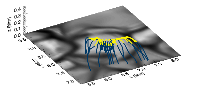
Figure 6: Trajectories of tracer fluid elements in the photospheric neighbourhood of a granule. The greyscale image in the $z=0$ plane shows the vertical velocity there at the time when the tracer fluid elements were released. The colour coding of the trajectories corresponds to the sign of the radiative heating $Q_{\rm rad}$ experienced by the fluid elements (dark blue means $Q_{\rm rad}<0$, yellow means $Q_{\rm rad}>0$).

Figure 6 shows a subvolume of the simulation domain in the neighbourhood of the granule centered at $[x,y]=[7,8]$ Mm in Fig. 3. The greyscale image at $z=0$ indicates the vertical velocity at $z=0$ at the instant when the tracer fluid elements were released ($t=0$). The colour-coding of the trajectories indicate the sign of $Q_{\rm rad}$: dark blue means $Q_{\rm rad}<0$ (cooling), yellow means $Q_{\rm rad}>0$ (heating). The set of trajectories resembles a fountain: the fluid elements originate from the granule interior, travel up to the photosphere and eventually overturn and descend into the downflow network in the convection zone.

3.3.1 The motion of fluid elements in the photosphere

First we concentrate on the motion and dynamics of the fluid elements. As Fig. 6 shows, in spite of the strongly stable average stratification, the fluid elements are able to penetrate into the photosphere. The shape of the trajectories tell us that in the photosphere, they experience a deceleration in the vertical direction and a deflection towards the edge of the granule.

In the following, we give a brief description of the force balance which drives the horizontal granular outflows and the feeding of the downflows in the intergranular lanes. Inspection of the horizontal pressure fluctuations in the photospheric layers of our simulation reveal that local pressure hills in the interior of granules are responsible for the buoyancy braking of the upflows and the deflection of material horizontally outwards from the centres of granules. At the interface between two granules, the horizontal outflows from the granules meet and develop localized pressure ridges. These localized regions of pressure enhancement serve to retard the horizontal granular outflows. So, when a fluid element in the granular outflow approaches the intergranular boundary, it is decelerated by the pressure gradient. Finally, the pressure enhancement at the boundaries, together with gravity, work in tandem to accelerate the fluid element downwards, thereby feeding the intergranular downflow network. These results are in accordance with results from 2D idealized simulations of compressible convection (Hurlburt & Toomre, 1988; Hurlburt, Toomre, & Massaguer, 1986) and 3D near-surface convection simulations (Nordlund, 1985; Stein & Nordlund, 1998).

3.3.2 The thermodynamic history of fluid elements in the photosphere

To avoid confusion in the following discussion, at this point we would like to clarify the following terminology: By heating (cooling), we refer to a non-adiabatic process which increases (decreases) the specific entropy of a fluid element. For example, when a fluid element absorbs more radiation than it emits, it is heated and gains entropy. A fluid element which is compressed adiabatically, however, will have a higher final temperature but is not heated. In the absence of viscous dissipation or thermal conduction, the equation governing the evolution of the specific entropy of a fluid element is

$$\frac{Ds}{Dt}=\frac{Q_{\rm rad}}{\varrho T},$$ (7)

where $D/Dt$ denotes the Lagrangian derivative (Mihalas & Mihalas, 1985). The corresponding equation governing the temperature of a fluid element is

$$\frac{D\ln{T}}{Dt} = (\gamma_{3}-1)\frac{D\ln{\varrho}}{Dt}+\left(\frac{\partial\ln{T}}{\partial s}\right)_{\varrho}\frac{Ds}{Dt}$$ (8)

$$= -(\gamma_{3}-1)\nabla\cdot\mathbf{v}+\left(\frac{\partial\ln{T}}{\partial s}\right)_{\varrho}\frac{Q_{\rm rad}}{\varrho T}.$$ (9)

where $\gamma_{3}=1+\left(\frac{\partial\ln{T}}{\partial\ln{\varrho}}\right)_{s}>1$ is Chandrasekhar’s third adiabatic exponent. Two effects contribute to changes in the gas temperature of a fluid element. The first term on the r.h.s. of Eq. (9) describes the role of adiabatic expansion or compression. Clearly, the effect of adiabatic expansion ($\nabla\cdot\mathbf{v}>0,~{}Q_{\rm rad}=0$) is to decrease the gas temperature. The second term on the r.h.s. of Eq. (9) describes the role of radiative heating. As expected, radiative heating (cooling) leads to an increase (decrease) of the gas temperature. The relative importance of the two effects in controlling the fluid temperature depends on their characteristic timescales. Inspection of Eq. (9) motivates us to define the dynamical and radiative timescales respectively as

$$t_{\rm dyn} = \left|\frac{1}{(\gamma_{3}-1)\nabla\cdot\mathbf{v}}\right|,{\rm~{}and}$$ (10)

$$t_{\rm rad} = \left|\left(\frac{\partial s}{\partial\ln{T}}\right)_{\varrho}\frac{\varrho T}{Q_{\rm rad}}\right|.$$ (11)

In the case that $t_{\rm dyn}\ll t_{\rm rad}$, the motion of a fluid element is essentially adiabatic. In the opposite extreme, where $t_{\rm dyn}\gg t_{\rm rad}$, the fluid element is always in radiative equilibrium with its surroundings.

Now we proceed to discuss the thermodynamic history of fluid elements overshooting into the photosphere. Owing to the large opacity for $z<0$, fluid in the upwellings in the convection zone ascend almost adiabatically. The decrease of a fluid element’s temperature during its rise in the convection zone is due to adiabatic expansion. As it approaches the photosphere, the opacity drops rapidly and the fluid element loses entropy by radiative cooling. Thereafter, the fluid element overshoots into the stably stratified photosphere. Although the fluid element is now optically thin, it is not completely transparent to radiation and continues to exchange energy with its surroundings. In regions above granules, (consisting of overshooting material), radiative energy exchange predominantly leads to heating. This effect can be seen in the colour-coding of the trajectories in Fig. 6. This figure clearly indicates that as the fluid elements penetrate into the photosphere (and as they are diverted toward the intergranular lanes), they experience radiative heating.

Stein & Nordlund (1998) also found that rising fluid in the photosphere is systematically reheated by the radiation field (see Fig. 18 of their paper). The reason for this behaviour is the thermostatic action of the radiation field to keep the fluid elements close to radiative equilibrium. The radiative equilibrium temperature $T_{\rm RE}$ of a fluid element embedded in a radiation field is defined as the temperature at which the fluid element emits and absorbs radiation in equal amounts (i.e. $Q_{\rm rad}=0$). One can make a simple estimate for the lower limit of $T_{\rm RE}$ by assuming the fluid element to be located at $\tau=0$. In the approximation of grey radiative transfer, $\kappa_{\nu}$ is replaced by the mean opacity $\bar{\kappa}$, so that Eq. (4) becomes

$$Q_{\rm rad}=4\pi\bar{\kappa}\varrho[J-B(T)],$$ (12)

where $B(T)=\int_{0}^{\infty}B_{\nu}(T){\rm d}\nu=(\sigma/\pi)T^{4}$ is the frequency-integrated Planck function and $J=(4\pi)^{-1}\int_{4\pi}\int_{0}^{\infty}I_{\nu}{\rm d}\nu{\rm d}\Omega$ is the angle-averaged, frequency-integrated intensity. Assume that the solar atmosphere has plane-parallel symmetry. In this case, $I_{\nu}$ is symmetric about the $z$-axis. Making use of the Eddington-Barbier approximation, we obtain

$$J = \frac{1}{4\pi}\int_{0}^{\infty}\oint_{4\pi}I_{\nu}{\rm d}\Omega{\rm d}\nu$$ (13)

$$= \int_{0}^{\infty}\left[\frac{1}{2}\int_{-1}^{1}B_{\nu}(T|_{\tau=\mu}){\rm d}\mu\right]{\rm d}\nu$$

$$= \frac{\sigma}{2\pi}\int_{-1}^{1}(T|_{\tau=\mu})^{4}{\rm d}\mu,$$

where $\mu=\vec{\mu}\cdot\mathbf{\hat{z}}=\cos{\theta}$. Here $\mathbf{\mu}$ is the direction cosine vector and $\theta$ is the angle between $\mathbf{\mu}$ and $\hat{z}$. By definition, $T_{\rm RE}$ is such that $B(T_{\rm RE})=(\sigma/\pi)T_{\rm RE}^{4}=J$. To evaluate $J$ from Eq. (13), we use the average temperature profile $\bar{T}(\tau)$ from our model. This yields $T_{\rm RE}=4600$ K. This result tells us why granular material ascending in the photosphere must be radiatively heated. Consider a fluid element that is rising in the photosphere. If the fluid element rises adiabatically, its temperature would drop so quickly with height, that it becomes cooler than the radiative equilibrium temperature. As soon as this happens, the fluid element will absorb more radiation than it emits ($Q_{\rm rad}>0$). By the same token, consider a fluid element in the photosphere which has been transported from the interior of a granule towards an intergranular lane. As it descends, it is compressed. If it were to descend adiabatically, its temperature would soon be above $T_{\rm RE}$, which means it must then cool radiatively.

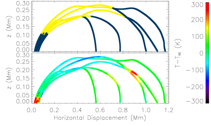
Figure 7: Upper panel: Trajectories are colour-coded according to the sign of $Q_{\rm rad}$ (dark blue and yellow correspond to $Q_{\rm rad}<0$ and $Q_{\rm rad}>0$, respectively). Lower panel: Trajectories are colour-coded according to the value of $T-T_{\rm RE}$, the deviation of the gas temperature from the radiative equilibrium temperature. In both panels, the fluid elements emanate from the left-hand-side and travel towards the right.

Figure 7 provides an illustration of how overshooting fluid elements become cooler than $T_{\rm RE}$ as they penetrate into the photosphere, and subsequently become hotter than $T_{\rm RE}$ as they descend towards the convection zone. In the figure, the height $z$ of a fluid element is plotted as a function of the horizontal displacement from its original position (i.e. $[\Delta x^{2}+\Delta y^{2}]^{1/2}$). In both panels, the fluid elements travel from the left to the right of the plot. In the upper panel, the trajectories are colour-coded according to the sign of $Q_{\rm rad}$. In the lower panel, they are colour-coded according to the instantaneous, local value of $T-T_{\rm RE}$. $T_{\rm RE}$ is evaluated by keeping track of $J_{i}$ and $\kappa_{i}$ ($i$ refers to the index of the frequency bin) along the trajectories and then finding a temperature $T$ such that $\sum\kappa_{i}B_{i}(T)=\sum\kappa_{i}J_{i}$.

As a rising fluid element approaches the base of the photosphere, its temperature can be up to $400$ K higher than $T_{\rm RE}$. This causes the fluid element to radiate intensely. Once the fluid element has reached the optically thin layers of the photosphere, adiabatic expansion and radiative heating compete to control the temperature of the fluid element. The relative importance of these two effects (measured by the ratio of $t_{\rm dyn}$ and $t_{\rm rad}$) determine whether the fluid element will be driven towards or away from radiative equilibrium. For a fluid element penetrating into the middle photosphere in a granular environment, we find that $0.1\lesssim t_{\rm dyn}/t_{\rm rad}\lesssim 1$. This means that the decrease in fluid temperature due to expansion of the fluid element is only partially compensated by radiative heating. Consequently, its temperature decreases and it departs further away from $T_{\rm RE}$. In Fig. 7, we can see a general trend for $T-T_{\rm RE}$ to become more negative as a fluid element rises. For fluid elements that penetrate beyond $z=250$ km, $T-T_{\rm RE}$ can reach a value of $-200$ K.

Figure 8 shows the profiles of $s$, $T$ and $\varrho$ along one of the trajectories shown in Fig. 6. The colour-coding indicates the sign of $Q_{\rm rad}$ experienced by the fluid element along its trajectory (dark blue means $Q_{\rm rad}<0$, yellow means $Q_{\rm rad}>0$). The motion of the fluid element before it emerged at the surface is essentially adiabatic, with $s=6.1R^{\star}$, where $R^{\star}$ is the universal gas constant. As it approaches $z\approx 0$, radiative cooling leads to a steep drop of $s$ and $T$ with height. Accompanying this cooling is a simultaneous compression of the fluid element, so that it becomes temporarily denser than the fluid beneath it. Thereafter, the fluid element continues to ascend and the density decreases again. When it has reached $z=0.1$ Mm, the fluid element is cooler than $T_{\rm RE}$ and it begins to be heated radiatively. This radiative heating leads to a rise in entropy, while the temperature continues to decrease because the effect of expansion overwhelms that of radiative heating. Finally, at $z=0.28$ Mm, the fluid element overturns and begins its descent. At this moment, the fluid element has a gas temperature below $T_{\rm RE}$, so that it continues to be heated radiatively even though its temperature rises by compression. Only at $z=0.26$ Mm ($\approx 20$ km below the apex of the fluid element’s trajectory) is the temperature of the fluid element above $T_{\rm RE}$ and $Q_{\rm rad}$ becomes negative.

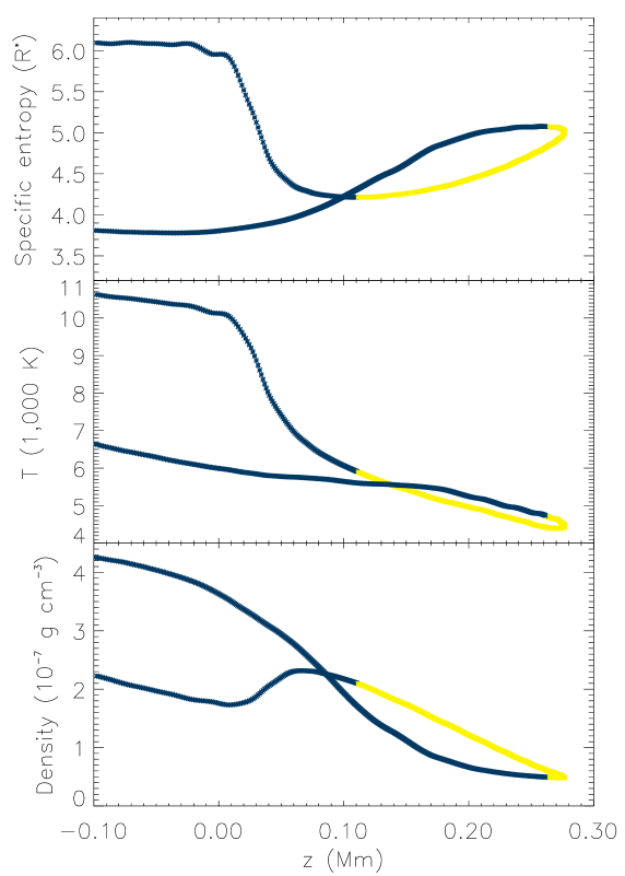
Figure 8: Profiles of specific entropy $s$, temperature $T$ and density $\varrho$ along one of the fluid element trajectories shown in Fig. 6. As the fluid element initially emerges at the base of the photosphere ($z\approx 0$), it has relatively high entropy, high temperature and low density. The colour-coding indicates the sign of $Q_{\rm rad}$ experienced by the fluid element along its trajectory (dark blue means $Q_{\rm rad}<0$, yellow means $Q_{\rm rad}>0$). Above $z=140$ km, the fluid element is hotter during descent than during its ascent. This is a result of radiative heating of the fluid element in the photosphere.

The profiles of $s$, $T$ and $\varrho$ in Fig. 8 exhibit hysteresis. There are two reasons for this behaviour. Firstly, there is a lag between when the fluid element overturns and when $Q_{\rm rad}$ switches sign (see previous paragraph). Secondly, the asymmetry in the speed of upflows (slower) and downflows (faster) means that the cumulative heating experienced by the fluid element over its journey upwards in the photosphere is greater than the accumulative radiative cooling it undergoes on the return journey. These two factors contribute to the temperature and entropy enhancements of the intergranular boundaries (downflows) with respect to the granules (upflows).

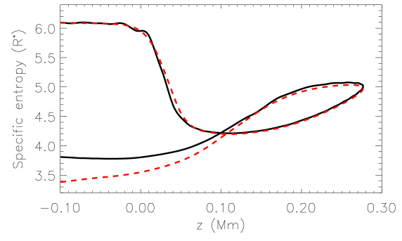
Figure 9: Reconstruction of specific entropy profile. The black solid curve shows the entropy profile as obtained by following the fluid element in the simulation (same as in the upper panel of Fig. 8). The red dashed curve shows the reconstructed entropy profile, $s_{\rm recon}$, calculated by integrating Eq. (7).

In order to test whether dissipative effects (viscous and thermal, e.g. in shocks) play a role in causing the temperature enhancement in the intergranular lanes in the upper photosphere, we have reconstructed the profiles of $s$ along the trajectory neglecting hyperdiffusivity effects. By keeping track of $Q_{\rm rad}(t)$, $\varrho(t)$ and $T(t)$ along the trajectory of a fluid element, we can reconstruct the time history of $s$ for a fluid element. Given these profiles and the initial entropy $s_{0}$ of the fluid element, Eq. (7) can be integrated to yield the reconstructed entropy profile $s_{\rm recon}(t)$. This quantity is plotted in Fig. 9 together with the entropy profile shown in Fig. 8. The good match of the two profiles in the layers $z\gtrsim 0$ tells us that radiation is indeed the cause of hysteresis in the entropy and temperature profiles. The reconstructed profile $s_{\rm recon}$ begins to deviate from the tracer profile once the fluid element approaches the narrow turbulent downflow jets in the convection zone. Here the radiative effects diminish and dissipative effects described by the hyperdiffusive terms become important.

4 Conclusion

The reversed granulation is a reversal of the pattern of intensity contrast between intensity maps in the continuum and intensity maps in spectral lines forming in the middle to upper photosphere. It has long been established that this reversal of the intensity fluctuations is a result of the sign change of the horizontal temperature fluctuations (see Fig. 5). Analysis of our 3D numerical model of the near-surface convection zone and photosphere confirms the existence of this reversal in the temperature fluctuations above a height of $z=130-140$ km, in agreement with previous observational findings.

By following in detail the time histories of fluid elements overshooting into the photosphere, we were able to identify the processes that determine the horizontal temperature fluctuations in the photosphere. We find that changes in the temperature of fluid elements in the photosphere result from adiabatic expansion and radiative heating. Whereas the former decreases the gas temperature of a fluid element, the latter increases it towards the radiative equilibrium temperature $T_{\rm RE}$. The ratio of the associated characteristic timescales tells us that, for a fluid element rising in the optically thin layers, the decrease of temperature due to expansion is only partially cancelled by radiative heating. This disparity allows a fluid element to depart from radiative equilibrium as it penetrates into the photosphere. Due to this deviation from $T_{\rm RE}$, a fluid element overturning in the optically thin layers still experiences some radiative heating as it begins to descend. This, together with the fact that downflows have higher vertical speed than upflows, leads to a hysteretic behaviour of the thermodynamic history of the fluid element (see Fig. 8).

In various guises in previous works, the following explanation has often been invoked to explain the origin of the reversal of temperature fluctuations: since the photosphere is subadiabatically stratified, material rising from granules into this stable layer has lower temperature that its ‘mean surroundings’. This view is problematic in two respects. Firstly, it implicitly assumes that material penetrating into the photosphere does so in an adiabatic fashion. Secondly, it is not at all clear what are the ‘mean surroundings’ of a fluid element embedded in convective flow consisting of disjointed upwellings separated by an intergranular network. Our present efforts highlight the importance of radiative energy exchange in the dynamics of the photosphere and helps dispel possible misconceptions regarding the origin of the reversed granulation in the photosphere.

Acknowledgements
MCMC thanks Prof. Franz Kneer and his group at the Georg-August University of Göttingen for valuable discussions on this topic. MCMC acknowledges financial support from the International Max Planck Research School at the Max Planck Institute for Solar System Research.

References

- Balthasar et al. (1990) Balthasar, H., Grosser, H., Schroeter, C., & Wiehr, E. 1990, A&A, 235, 437
- Borrero & Bellot Rubio (2002) Borrero, J. M. & Bellot Rubio, L. R. 2002, A&A, 385, 1056
- Caunt & Korpi (2001) Caunt, S. E. & Korpi, M. J. 2001, A&A, 369, 706
- Espagnet et al. (1995) Espagnet, O., Muller, R., Roudier, T., Mein, N., & Mein, P. 1995, A&AS, 109, 79
- Evans & Catalano (1972) Evans, J. W. & Catalano, C. P. 1972, Sol. Phys., 27, 299
- Hurlburt & Toomre (1988) Hurlburt, N. E. & Toomre, J. 1988, ApJ, 327, 920
- Hurlburt et al. (1986) Hurlburt, N. E., Toomre, J., & Massaguer, J. M. 1986, ApJ, 311, 563
- Janssen & Cauzzi (2006) Janssen, K. & Cauzzi, G. 2006, A&A, 450, 365
- Kucera et al. (1995) Kucera, A., Rybak, J., & Woehl, H. 1995, A&A, 298, 917
- Leenaarts & Wedemeyer-Böhm (2005) Leenaarts, J. & Wedemeyer-Böhm, S. 2005, A&A, 431, 687
- Lekien & Marsden (2005) Lekien, F. & Marsden, J. 2005, International Journal for Numerical Methods in Engineering, 63
- Mihalas & Mihalas (1985) Mihalas, D. & Mihalas, B. W. 1985, Foundations of Radiation Hydrodynamics (Oxford University Press, USA, 640 p.)
- Nordlund (1984) Nordlund, A. 1984, in Small-Scale Dynamical Processes in Quiet Stellar Atmospheres, ed. S. L. Keil, 181
- Nordlund (1985) Nordlund, A. 1985, Sol. Phys., 100, 209
- Puschmann et al. (2005) Puschmann, K. G., Ruiz Cobo, B., Vázquez, M., Bonet, J. A., & Hanslmeier, A. 2005, A&A, 441, 1157
- Rast et al. (1993) Rast, M. P., Nordlund, A., Stein, R. F., & Toomre, J. 1993, ApJ, 408, L53
- Rast & Toomre (1993) Rast, M. P. & Toomre, J. 1993, ApJ, 419, 224
- Rodríguez Hidalgo et al. (1999) Rodríguez Hidalgo, I., Ruiz Cobo, B., Collados, M., & del Toro Iniesta, J. C. 1999, in ASP Conf. Ser. 173: Stellar Structure: Theory and Test of Connective Energy Transport, ed. A. Gimenez, E. F. Guinan, & B. Montesinos, 313
- Ruiz Cobo et al. (1996) Ruiz Cobo, B., del Toro Iniesta, J. C., Rodriguez Hidalgo, I., Collados, M., & Sanchez Almeida, J. 1996, in ASP Conf. Ser. 109: Cool Stars, Stellar Systems, and the Sun, ed. R. Pallavicini & A. K. Dupree, 155
- Rutten et al. (2004) Rutten, R. J., de Wijn, A. G., & Sütterlin, P. 2004, A&A, 416, 333
- Spruit (1974) Spruit, H. C. 1974, Sol. Phys., 34, 277
- Steffen et al. (1989) Steffen, M., Ludwig, H.-G., & Krüss, A. 1989, A&A, 213, 371
- Stein & Nordlund (1998) Stein, R. F. & Nordlund, A. 1998, ApJ, 499, 914
- Suemoto et al. (1987) Suemoto, Z., Hiei, E., & Nakagomi, Y. 1987, Sol. Phys., 112, 59
- Suemoto et al. (1990) Suemoto, Z., Hiei, E., & Nakagomi, Y. 1990, Sol. Phys., 127, 11
- Title et al. (1989) Title, A. M., Tarbell, T. D., Topka, K. P., et al. 1989, ApJ, 336, 475
- Vögler (2003) Vögler, A. 2003, Three-dimensional simulations of magneto-convection in the solar photosphere (Göttingen University, http://webdoc.sub.gwdg.de/diss/2004/voegler/)
- Vögler (2004) Vögler, A. 2004, A&A, 421, 755
- Vögler et al. (2005) Vögler, A., Shelyag, S., Schüssler, M., et al. 2005, A&A, 429, 335