Imaging of star clusters in unperturbed spiral galaxies with the Advanced Camera for Surveys

Abstract

Context. Star clusters are present in almost all types of galaxies. Here we investigate the star cluster population in the low-luminosity, unperturbed spiral galaxy NGC 45, which is located in the nearby Sculptor group. Both the old (globular) and young star-cluster populations are studied.

Aims. Previous ground-based observations have suggested that NGC 45 has few if any “massive” young star clusters. We aim to study the population of lower-mass “open” star clusters and also identify old globular clusters that could not be distinguished from foreground stars in the ground-based data.

Methods. Star clusters were identified using $UBVI$ imaging from the Advanced Camera for Surveys (ACS) and the Wide Field Planetary Camera 2 (WFPC2) on board the Hubble Space Telescope. From broad band colors and comparison with simple stellar population (SSP) models assuming a fixed metallicity, we derived the age, mass, and extinction. We also measured the radius for each star cluster candidate.

Results. We identified 28 young star cluster candidates. While the exact values of age, mass, and extinction depend somewhat on the choice of SSP models, we find no young clusters with masses higher than a few 1000 $M_{\odot}$ for any model choice. We derive the luminosity function of young star clusters and find a slope of $\alpha=-1.94\pm 0.28$. We also identified 19 old globular clusters, which appear to have a mass distribution that is roughly consistent with what is observed in other globular cluster systems. Applying corrections for spatial incompleteness, we estimate a specific frequency of globular clusters of $S_{N}$=1.4–1.9, which is significantly higher than observed for other late-type galaxies (e.g. SMC, LMC, M33). Most of these globular clusters appear to belong to a metal-poor population, although they coincide spatially with the location of the bulge of NGC 45.

1 Introduction

Especially since the launch of the HST, young star clusters have been observed in an increasing variety of environments and galaxies. This includes interacting galaxies such as NGC 1275 (e.g. Holtzman et al. 1992), the Antennae system (e.g. Whitmore & Schweizer 1995), tidal tails (e.g. Bastian et al. 2005b), but also some normal disk galaxies (e.g. Larsen 2004). This shows that star clusters are common objects that can form in all star-forming galaxies. It remains unclear what types of events trigger star cluster formation and the formation of “massive” clusters in particular. It has been suggested that (at least some) globular clusters may have been formed in galaxy mergers (Schweizer 1987), and the observation of young massive star clusters in the Antennae and elsewhere may be an important hint that this is indeed a viable mechanism, although not necessarily the only one. In the case of normal spiral galaxies, spiral arms may also stimulate the molecular cloud formation (Elmegreen 1994) and thus the possibility of star cluster formation.

While a large fraction of stars appear to be forming in clusters initially, many of these clusters ( $\sim$90%) will not remain bound after gas removal and disperse after $\sim 10^{7}$ years (Whitmore 2003). This early cluster disruption may be further aided by mass loss due to the stellar evolution and dynamical processes (Fall 2004), so that many stars initially born in clusters eventually end up in the field.

Much attention has focused on star clusters in extreme environments such as mergers and starbursts, but little is currently known about star and star cluster formation in more quiescent galaxies, such as low-luminosity spiral galaxies. The Sculptor group is the nearest galaxy group, and it hosts a number of late-type galaxies with luminosities similar to those of SMC, LMC, and M33 (Cote et al. 1997). One of the outlying members is NGC 45, a low surface-brightness spiral galaxy with M${}_{B}=-17.13$ and distance modulus $(m-M)=28.42\pm 0.41$ (Bottinelli et al. 1985). This galaxy was included in the ground-based survey of young massive clusters (YMCs) in nearby spirals of Larsen & Richtler (1999), who found only one cluster candidate. Several additional old globular cluster candidates from ground-based observations were found by Olsen et al. (2004), but none of them has been confirmed.

In this paper we aim at studying star cluster formation in this galaxy using the advantages of the HST space observations. We identify star clusters through their sizes, which are expected to be stable in the lifetime of the cluster (Spitzer 1987). Then we derive their ages and masses using broadband colors with the limitations that this method implies, such as models dependences (de Grijs et al. 2005). Also we study how the choice of model metallicities affects our results.

This paper is structured in the following way, beginning in Sect. 2, we describe the observations, reductions, photometry, aperture corrections and, artificial object experiments. In Sect. 3, we describe the selection of our cluster candidates, the color magnitude diagram and their spatial distribution. In Sect. 4 we describe the properties of young star clusters. In Sect. 5 we comment on the globular cluster properties, and Sect. 6 contains the discussion and conclusions.

2 Data and reductions

Two different regions in NGC 45 were observed with the HST ACS Wide Field Channel on July 5, 2004. One pointing included the center of the galaxy ($\alpha_{2000}=00^{h}14^{m}0^{s}.30$, $\delta_{2000}=-23^{\circ}10\arcmin 04\arcsec$) and the other covered one of the spiral arms ($\alpha_{2000}=00^{h}14^{m}14^{s}.90$, $\delta_{2000}=-23^{\circ}12\arcmin 29\arcsec$). For each frame, two exposures of 340 seconds each were acquired through the filters F435W ($\sim B$) and F555W ($\sim V$), and a pair of 90 and 340 seconds was obtained through the filter F814W ($\sim I$). In addition, for each pointing, two F336W ($\sim U$-band) exposures of 1200 s each were taken with the WFPC2. The ACS images are shown in Fig. 1, including the footprint of the WFPC2 exposures. Due to the smaller field-of-view of WFPC2, only part of the ACS frames have corresponding $U$-band imaging.

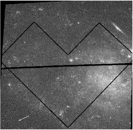
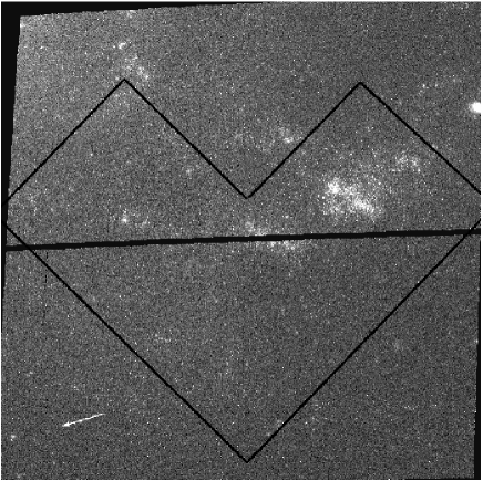
Figure 1: The two ACS images of NGC 45 with the HST WFPC2 (F336W) pointings also indicated. The arrows indicate the north.

Following standard “on-the-fly” pipeline processing, the raw ACS images were drizzled using the MULTIDRIZZLE task (Koekemoer et al. 2002) in the STSDAS package in IRAF. For most of the parameters in Multidrizzle we used the default values. However, we disabled the automatic sky subtraction, because did not work well for our data, due to the highly non-uniform background level. The WPFC2 images were combined using the CRREJ task and standard parameter settings.

2.1 Photometry

The source detection was carried out in the ACS $F435W$ images using SExtractor V2.4.3 (Bertin & Arnouts 1996). The object coordinates measured in the $B_{F435W}$ frame were used as input for the SExtractor runs on the other two ACS frames. An area of 5 connected pixels, all of them are more than 4 sigma above the background, was defined as an object. From the output of SExtractor we kept the FWHM measured in each filter and the object coordinates.

Aperture photometry was done with the PHOT task in IRAF, using the SExtractor coordinates as input. This was preferred over the SExtractor magnitudes because of the greater flexibility in DAOPHOT for choosing the background subtraction windows. We used an aperture radius of 6 pixels for the ACS photometry, which matches the typical sizes of star clusters well at the well distance of NGC 45 (1 ACS/WFC pixel $\sim$ 1.2 pc). The sky was subtracted using an annulus with inner radius of 8 pixels and a 5 pixel width.

Because the $U_{F336W}$ exposures were not as deep as the ACS exposures, we used the ACS object coordinates transformed into the WFPC2 frame in order to maximize the number of objects for which $U_{F336W}$ photometry was available. We defined a transformation between the ACS and WFPC2 coordinate systems using the GEOMAP task in IRAF, and transformed the ACS object lists to the WFPC2 frame with the GEOXYTRAN task. Each transformation typically had an rms of 0.5 pixels. The transformed coordinates were used as input for the WFPC2 aperture photometry. We used a 3 pixel aperture radius, which is the same physical aperture as in the ACS frames. The counts were converted to the Vega magnitude system using the HST zero-points taken form the HST web page and based on the spectrophotometric calibration of Vega from Bohlin & Gilliland (2004).

We identified a total of 14 objects in common with the ACS data and the WFPC2 chips. For the Planetary Camera (PC), we were not able to find any common objects to determine the correct transformation.

Figure 2: Photometry errors of the detected sources. The aperture radii used for the photometry are 6 pixels for the ACS data and 3 pixels for WFPC2.

2.2 Object sizes

Measuring object sizes is an important step in disentangling stars from extended objects. We performed size measurements on the ACS data. For this purpose we used the ISHAPE task in BAOLAB (Larsen 1999). ISHAPE models a source as an analytical function (in our case, King 1962 profiles) convolved with the PSF. For each object Ishape starts from an initial value for the FWHM, ellipticity, orientation, amplitude, and object position, which are then used in an $\chi^{2}$ iterative minimization. The output includes the derived FWHM, chi-square, flux, and signal-to-noise for each object plus a residual image. A King concentration parameter of c=30, fitting radius of 10 pixels, and a maximum centering radius of 3 pixels were adopted as input parameters for Ishape. These results are described in Sect. 3.

2.3 Aperture corrections

Aperture corrections from our photometric apertures to a reference ($1\aas@@fstack{\prime\prime}45$) aperture should ideally be derived using the same objects in all the frames. Those objects should be extended, isolated, and easily detectable. In our case this was impossible because most of the objects were not isolated, and the few isolated ones were too faint in the WFPC2 frame. For this reason, we decided to create artificial extended objects and derive the aperture corrections from them. We proceed for the ACS as follows.

First, we generated an empirical PSF for point sources in the ACS images, using the PSF task in DAOPHOT running within IRAF. Since we want to be sure that we are only selecting stars in the PSF construction, we used ACS images of the Galactic globular cluster 47 Tuc . We selected 139, 84, and 79 stars through the $B_{F435W}$, $V_{F555W}$, and $I_{F814W}$ filters with 10 sec, 150 sec, and 72 sec of exposure time, respectively. We could not use the same objects in all the filters because the ACS frames have different pointings and exposure times. The selected stars were more or less uniformly distributed over the CCD, but we avoided the core of the globular cluster because stars there were crowded and saturated. We used a PSF radius of 11 pixels and a fitting radius of 4 pixels on each image. This was the maximum possible radius for each star without being affected by the neighboring one.

Second, models of extended sources were generated using the baolab MKCMPPSF task (Larsen 1999). This task creates a PSF by convolving a user-supplied profile (in our case the empirical ACS PSF) with an analytical profile (here a King 1962 model with concentration parameter $r_{\rm tidal}/r_{\rm core}=30$) with a FWHM specified by the user. The result is a new PSF for extended objects.

Third, we used the MKSYNTH task in BAOLAB to create an artificial image with artificial extended sources on it.

For the WFPC2 images we proceeded in a similar way, but we used the Tiny Tim (Krist 1993) package for the PSF generation. We kept the same PSF diameter as for the ACS images. We then followed the same procedure as for the ACS PSF. Aperture corrections were done taken into account the profile used for size measurements (King30) and the size derived from it for each object. Since sizes were measured in the ACS frames, we assumed that objects in the WFPC frames have similar sizes. Aperture corrections were corrected from 6 pixels for the ACS data and 3 pixels for WFPC2 to a nominal $1\aas@@fstack{\prime\prime}45$ (where aperture corrections start to remain constant) reference aperture. The corrections are listed in Table 1

Table 1: Aperture corrections as a function of object size (FWHM).

$$\begin{array}[]{ccccc}\hline\cr\hline\cr\vskip 3.0pt plus 1.0pt minus 1.0pt\cr(1)&(2)&(3)&(4)&(5)\\ FWHM(pix)&U_{F336W}[mag]&B_{F435W}[mag]&V_{F555W}[mag]&I_{F814W}[mag]\\ &WFPC2&ACS&ACS&ACS\\ \hline\cr 0.20-0.75&-0.050&-0.053&-0.046&-0.054\\ 0.75-1.50&-0.168&-0.167&-0.153&-0.163\\ 1.50-2.15&-0.358&-0.343&-0.337&-0.345\\ 2.15-2.75&-0.517&-0.506&-0.491&-0.505\\ \vskip 3.0pt plus 1.0pt minus 1.0pt\cr\hline\cr\end{array}$$

Colors do not change significantly as a function of size. From Table 1, we note that an error in size will be translated into a magnitude error: e.g. 0.3 pixel of error in the measured FWHM correspond to $\Delta m=0.07$ which, translated into mass, corresponds to a $7\%$ error. We also keep in mind that adopting an average correction over each small size ranges (0.20-0.75, 0.75-1.50, 1.50-2.15, 2.15-2.75) and introduce an additional uncertainty in mass of $\sim 8\%$

The other systematic effect on our measurements is that aperture correction changes for the different profiles. We adopt a King30 profile, fitting most of our objects best. For comparison we give some examples of the effect below. For an object of FWHM=0.5 pixels, the aperture correction varies from $\Delta m=-0.036$ [mag] ($3\%$ in mass) considering a KING5 profile up to $\Delta m=-0.205$ [mag] ($17\%$ in mass) considering a King100 profile. For an object of FWHM=1.2 pixels, the aperture correction varies from $\Delta m=-0.045$ [mag] using King5 ($4\%$ in mass), up to $\Delta m=-0.437$ [mag] ($35\%$ in mass) considering a King100 profile. And for an object of FWHM=2.5 pixels, the aperture correction varies from $\Delta m=-0.078$ ($7\%$ in mass) considering a King5 profile up to $\Delta m=-0.645$ [mag] ($45\%$ in mass) considering a King100 profile. Thus in general the exact size and assumed profiles will cause errors in mass.

2.4 Artificial object experiments

We need to estimate the limits of our sample’s reliability in magnitudes and sizes. In the following we investigate how factors such as the degree of crowding and the background level affect the detection process and size derivation. To do so, we added 100 artificial objects and repeated the analysis for 3 different sub-regions in the ACS images: “field I” was centered on the bulge of the galaxy, “field II” included a crowded region with many young stars, and “field III’ covered a low-background region far from the center of the galaxy (see Fig. 3). Each field measured 1000 x 1000 pixels, and the artificial objects were distributed in an array of 10 by 10. A random shift between 0 and 20 pixels was added to the original object positions.

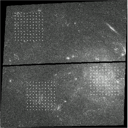
Figure 3: Artificial objects added to the science image. The three different test fields are shown, starting from the right and going clockwise: Field I (high background, and crowded background), Field II (young star-forming region), Field III (low background region).

In this way, the minimum separation between objects is 60 pixels.

The artificial objects were built using an artificial PSF as described in the second step of the aperture correction. Objects with a fixed magnitude were then added to a zero-background image (as in the third step of aperture correction). Finally we added this image, containing the artificial objects, to the science image using the IMARITH task in IRAF. This was done for objects with magnitudes between m($B_{F435W}$)=16 and m($B_{F435W}$)=26 and different FWHM (0.1 pixels (stars), 0.5, 0.9, 1.2, 1.5, and 1.8 pixels). The recovering process was performed in exactly the same way as for the original science object detections (SExtractor detection, aperture photometry, and Ishape run).

Figure 4: Completeness profiles for each of the test “fields” in the ACS image. The different lines represent different FWHMs.

Figure 4 shows the fraction of artificial objects recovered as a function of magnitude for different intrinsic object sizes and for each of the three test fields. As expected, the completeness tests show that more extended objects are more difficult to detect at a fixed magnitude. Fields II and III show very similar behavior, perhaps not surprisingly, since the crowded parts of field II cover only a small fraction of the test field. The higher background level in Field I results in a somewhat shallower detection limit, but for all the fields the 50% completeness limit is reached between m($B_{F435W}$)=25 and m($B_{F435W}$)=26.

Figure 5: Absolute value of the average of the input FWHM and the recovered value for each magnitude on each field. Faintest magnitudes show biggest FWHMs differences. The 0 $\sigma$ observed in the fields II and III at $B_{F435W}\sim 25.5$ means that no objects were recovered in these bins.

The artificial object experiments also allow us to test the reliability of the size measurements. In Fig.  5 we plot the average value of the absolute difference between the input FWHM and the recovered FWHM as a function of magnitude for the three different fields. More extended clusters show bigger absolute differences between the input and output FWHM at fixed magnitude compared with the less extended. Uncertainties are generally larger in the crowded and high background regions. In Field 1, the artificial object tests give an average difference between the input FWHM and the recovered one of $\sigma$=$0.006$ pixels for an object with m($B_{F435W}$)$=$20 and FWHM(input)=0.5 pixels. The corresponding errors at m($B_{F435W}$)=23 and m($B_{F435W}$)=24 are $\sigma$=$0.06$ pixels and $\sigma$=$0.12$ pixels, and a 50% error ($\sigma$=$0.25$ pixels) is reached at m($B_{F435W}$)$\sim$25. The relative errors also remain roughly constant at a fixed magnitude for more extended objects; for FWHM=$1.8$ pix the 50% error limit is at m($B_{F435W}$)=24.6.

3 Selection of cluster candidates

For the selection of star cluster candidates, we took advantage of the excellent spatial resolution of the ACS images. At the distance of NGC 45, one ACS pixel ($0\aas@@fstack{\prime\prime}05$) corresponds to a linear scale of about 1.2 pc. With typical half-light radii of a few pc (e.g. Larsen 2004), young star clusters are thus expected to be easily recognizable as extended objects. However, the high spatial resolution and depth of the ACS images also add a number of complications: as discussed in the previous section, our detection limit is at $B\sim 25.5$, or $M_{B}\sim-3$ at the distance of NGC 45. Clusters of such low luminosities are often dominated by a few bright stars, so it can be difficult to distinguish between a true star cluster and chance alignments of individual field stars along the line-of-sight. Therefore, we limit ourselves to brighter objects for which reliable sizes can be measured. We adopt a magnitude limit of m($B_{F435W}$)=23.2, corresponding to $M_{B}\sim 5.5$ and to a size uncertainty of $\sim 20$% for objects with FWHM $\leq 2.5$ pixel. Only one object (ID=9) has a larger FWHM than this.

Figure 6: Histogram of the size distributions from ISHAPE with a zoom in to the extended objects (bottom) and SExtractor (top). The dotted line shows the size selection criteria.

In an attempt to improve our object detection scheme, we use both size estimates from ISHAPE and SExtractor. In Fig. 6 we plot the distribution of size measurements for all the objects with $B_{F435W}\leq 23.2$.

The SExtractor sizes show a peak around FWHM$\sim$2.5, corresponding to the PSF FWHM, while the ISHAPE distribution peaks at 0 (recall that the ISHAPE sizes are corrected for the PSF). We adopt the size criteria of $FWHM_{\rm SEx}\geq 2.7$ and $FWHM_{\rm ISHAPE}\geq 0.2$ to select extended objects. In Fig. 7 we plot all objects with at least one condition fulfilled. From this figure it is evident that several objects were considered to be extended according to the SExtractor sizes, while the ISHAPE fit yield to near-zero size. Such objects might be close groupings of stars where SExtractor yields the size of the whole group, while ISHAPE fits a single star. On the other hand, there are very few objects that are classified as extended by ISHAPE but as compact according to SExtractor.

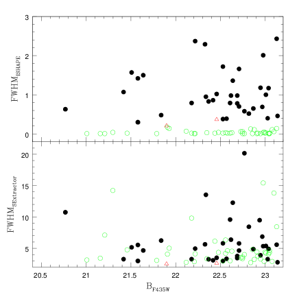
Figure 7: Object FWHMs as measured by ISHAPE and SExtractor. Filled circles are objects considered extended by both methods. Open circles were considered as extended objects only by SExtractor and triangles are objects considered extended only by ISHAPE.

Objects that fulfill both conditions are considered to be star cluster candidates. Objects that fulfill only one condition are considered to be possible clusters. Objects that did not pass any condition were rejected (i.e. classified as stars). All the objects were visually inspected to avoid contamination by HII regions. Finally 66 objects were rated as star cluster candidates and 64 as possible clusters, while 59 of these “possible” star cluster were considered as stars by ISHAPE and 2 as stars by SExtractor. From the 66 star cluster candidates, 36 have 4-band photometry and 30 have only ACS (3-band) photometry. In the following, only star cluster candidates are considered for the analysis.

3.1 Young clusters vs globular clusters

In Fig. 8 the color magnitude diagrams are shown for star clusters candidates and possible clusters.

Figure 8: Color-magnitude diagram for objects in NGC 45. The left side corresponds to all objects with $B_{F435W}$,$V_{F555W}$ and, $I_{F814W}$ ACS photometry and the right side correspond to objects with 4-band photometry (ACS filters plus $U_{F336W}$ from WFPC2). Filled circles are extended objects (i.e. star clusters) selected by SExtractor and Ishape, while open circles are objects that did not pass one of the size selection criteria. The dashed line is the TO of the old MW globular clusters system M${}_{V,TO}\sim-7.4$.

Two populations can be distinguished: A population of blue (and probably young) objects with $V_{F555W}-I_{F814W}\leq 0.8$ (with a main concentration around $V_{F555W}-I_{F814W}\sim 0$), and a red population $V_{F555W}-I_{F814W}\geq 0.8$, concentrated around $V_{F555W}-I_{F814W}\sim 1$ (globular clusters). Two blue clusters brighter than $V_{F555W}=21$ ($M_{V}\sim-7.5$) are found. The red objects have colors consistent with those expected for old globular clusters and are all extended according to both the SExtractor and ISHAPE size criteria.

Figure 9: Star cluster spatial distribution from the center of the galaxy at different radius. Top: Cumulative distribution with radius. Bottom: Number of objects per radius and globular cluster spatial completeness.

The spatial distribution is shown in Fig. 9 for all the clusters with 3-band photometry (ACS field of view). Globular clusters are concentrated towards the center of the galaxy, and their number decreases with their distance. In contrast, young clusters are distributed in the outer part of the galaxy showing 2 major concentrations at 78 arcsec and 190 arcsec. Young clusters are associated with star forming regions, therefore it is more likely to find them in spiral arms like the first concentration rather than in the center. The second concentration corresponds mainly to the clusters detected in the second pointing covering one of the spirals arms and young regions.

Spatial completeness is $100\%$ up to 20 arcsec radius. Beyond 20 arcsec, the completeness drops down to $20\%$ at 200 arcsec radius. For all completeness corrections, we assume the non-covered areas to be similar to the covered area in all respects.

The detection of young and globular star clusters do not vary differentially with radius. Therefore the central concentration of the globular clusters is not an artifact of detection completion.

Assuming that the covered area is representative of the non-covered area and that the number and distribution of star clusters are similar in the non-covered area, we expect that the observed tendency of globular clusters being located towards the center of the galaxy and the young ones toward the outer parts will remain.

In the following we discuss the young clusters and globular clusters separately. Our sample includes 36 star clusters with UBVI data (28 young star clusters and 8 globular clusters) and 11 globular clusters with BVI data. We will not discuss further the ages nor masses derived for the globular clusters since they are unreliable due to their faint $U_{F336W}$ band magnitudes. Only for completeness we show their derived ages and masses in the table 3.

4 Young star clusters

In this section, we discuss the properties of young clusters in more detail.

4.1 Colors

Figure 10: Color-color diagram of NGC 45 star cluster candidates, uncorrected for reddening. Each line corresponds to SSP GALEV models of different metallicities for a Salpeter IMF and ages from 1 Myr up to 10 Gyr. The arrow corresponds to an extinction of 1 mag.

The $U_{F336W}-B_{F435W}$ vs. $V_{F555W}-I_{F814W}$ two-color diagram of NGC 45 young star cluster candidates (not reddening corrected) is shown in Fig. 10. Also shown in the figure are GALEV (Anders & Fritze-v. Alvensleben 2003) SSP models for different metallicities. Age increases along the tracks from blue towards redder colors. The “hook” at $V_{F555W}-I_{F814W}$$\sim 0.5$ and $U_{F336W}-B_{F435W}$$\sim-1$ corresponds to the appearance of red supergiant stars at $\sim 10^{7}$ years and is strongly metallicity dependent. Many of the clusters have colors consistent with very young ages ($<10^{7}$ years), and some older cluster candidates are spread along the theoretical tracks.

The cluster colors show a considerable scatter compared with the model predictions, significantly larger than the photometric errors. For younger objects, the scatter may be due to random fluctuations in the number and magnitude of red supergiant stars present in each cluster (Girardi et al. 1995). Reddening variations can also contribute to the scatter, and for the older clusters ($\ga$ 1 Gyr), metallicity effects may also play a role since the models in each panel follow a fixed metallicity.

Generally, the cluster colors seem to be better described by models of sub-solar metallicity (Z=0.004 and Z=0.008). Considering that the luminosity of NGC 45 is intermediate between those of the small and large Magellanic clouds, we might indeed expect young clusters to have intermediate metallicities between those typical of young stellar populations in the Magellanic clouds.

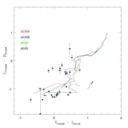
Figure 11: Reddening-corrected color-color diagram of NGC 45 star clusters. Each cluster was corrected according to the lowest $\chi^{2}$ metallicity-fitted model. All the theoretical tracks are plotted for 4 different metallicities. See Tables 2 and 3 for the derived values.

4.2 Ages and masses

One of main problems in deriving ages, metallicities, and masses for star clusters in spirals is that we do not know the extinction towards the individual objects. Bik et al. (2003) propose a method known as the “3D fitting” method to solve this problem. This method estimates the extinction, age, and mass by assuming a fixed metallicity for each single cluster. The method relies on a SSP model (in our case GALEV assuming a Salpeter IMF, Anders & Fritze-v. Alvensleben 2003), which provides the broad-band colors as a function of age and metallicity. The algorithm compares the model colors with the observed ones and searches for the best-fitting extinction (using a step of 0.01 in $E(B-V)$) and age for each cluster, using a minimum $\chi^{2}$ criterion. Finally the mass is estimated by comparing the mass-to-light ratios predicted by the models (for a fixed metallicity) with the observed magnitudes.

In Fig. 11 we plot the model tracks for 4 metallicities, together with the cluster colors corrected for reddening, according to the best $\chi^{2}$ fitting for the different metallicities. The 3D fitting method will move the clusters in the opposite direction with respect to the reddening arrow in Fig. 11, finding the closest matching model.

From Hyperleda (Paturel et al. 2003), the internal extinction in B-band for NGC 45 is $A_{B}=0.34$, based on the inclination and the morphological galaxy type taken from Bottinelli et al. (1995). Assuming $A_{B}=1.324*A_{V}$ from Rieke & Lebofsky (1985), we expect $E(B-V)\sim 0.08$. The mean derived extinction for the clusters is $E(B-V)=0.04$ for $Z=0.008$ and $Z=0.004$, $E(B-V)=0.05$ for $Z=0.02$, and $E(B-V)=0.1$ for $Z=0.05$. These values agree well with our derived value. Considering that some clusters lie in the foreground and some in the background, the extinction value from the literature agrees well with the extinctions we derive for our star clusters.

The 3D fitting method was applied for all clusters with 4-band photometry assuming in turn for different metallicities (Z=0.004, Z=0.008, Z=0.02, and Z=0.05). To explore how the assumed metallicity affects the derived parameters, we plot the cluster masses in Fig. 12 against cluster ages for all the models. In a general overview of each plot we see concentrations of clusters around particular ages, e.g. near $\log(Age/yr)\sim 7.2$ and $\sim 8$ in the Z=0.008 plot. These concentrations are not physical, but instead artifacts due to the model fitting (see Bik et al. 2003). In particular, the concentration around $log(Age/yr)\sim 7$ is due to the rapid change in the integrated cluster colors at that age (corresponding to the “hook” in Fig. 10). The figure again illustrates that the exact age at which this feature appears is metallicity dependent.

Independent of metallicity, Fig. 12 shows a concentration of young and not very massive clusters ($M\la 10^{3}M_{\odot}$) around $10^{6.8}$ yr. At older ages, the number of detected cluster candidates per age bin (note the logarithmic age scale) decreases rapidly. This is a result of fading due to stellar evolution (as indicated by the solid lines), as well as cluster disruption (see Sect. 4.4).

Figure 12: Mass as a function of cluster age. All star cluster candidates with masses greater than 100 solar masses are plotted here. Filled circles are young clusters. The lines represent a cluster of $F435W=23.1$ at different ages and masses for each metallicity.

4.3 Sizes

The young cluster candidates detected in NGC 45 are generally low-mass, compact objects. The average size (from ISHAPE) is FWHM=1.16 $\pm$ 0.2 pixel, equivalent to a half-light radius of R_eff= 2.0 $\pm$ 0.2 pc (errors are the standard error of the mean). These mean sizes are somewhat smaller than those derived by Larsen (2004) for clusters in a sample of normal spiral galaxies, which typically range from 3–5 pc. Previous work on star clusters has shown that there is at most a shallow correlation between cluster sizes and masses. For example, young star clusters found in NGC 3256 by Zepf et al. (1999) and by Larsen (2004) in a sample of nearby spiral galaxies show a slight correlation between their radii and masses, although Bastian et al. (2005a) do not find any apparent relation between radii and masses in M51. Larsen (2004) derived the following relation between cluster mass and size: $R_{\rm eff}=1.12\times(M/M_{\odot})^{0.10}$ pc. For a cluster mass of $10^{3}$ M_⊙, which is more typical of the young clusters observed here, this corresponds to a mean size of 2.2 pc. Thus, the difference between the cluster sizes derived by other studies of extragalactic star clusters and those found for NGC 45 here may be at least partly due to the lower cluster masses encountered in NGC 45. Of course, biases in the literature studies also need to be carefully considered. For example, Larsen (2004) excludes the most compact objects, which might cause the mean sizes to be systematically overestimated in that study.

Figure 13 shows the effective radius versus mass and age for the cluster candidates in NGC 45 (mass estimates are for Z=0.008). The plotted line is the best-fitting relation of the form :

$$R_{eff}=a*M^{b}$$ (1)

where $a=0.24$ $\pm$ $0.16$ and $b=0.29\pm 0.08$ are the best-fitting values. As in previous studies, there is a slight tendency for the more massive clusters to have larger sizes, but our fit has a large scatter and the constants are not tightly constrained. Therefore we suggest that the NGC 45 sample cannot be taken as strong evidence of a size-mass relation, but it does not contradict the general shallow trends found in other studies.

Figure 13: Effective radius vs mass (top) and age (bottom). The curve on top is the fitting of a power-law $R_{eff}=a*M^{b}$

4.4 Cluster disruption time

Boutloukos & Lamers (2003) defined the disruption time as

$$t_{dis}(M)=t_{4}^{dis}(M/10^{4}M_{\odot})^{\gamma},$$ (2)

where $t_{4}^{dis}$ is the disruption time of a cluster with an initial mass of $10^{4}M_{\odot}$. The constant $\gamma$ has been found empirically to have a value of about $\gamma=0.6$ (Boutloukos & Lamers 2003). If a constant number of clusters are formed per unit time (constant cluster formation rate) and clusters are formed in a certain mass range with a fixed cluster initial mass function (CIMF), which can be written as a power law

$$N(M)\sim M^{-\alpha},$$ (3)

then the number of clusters (per age interval) detected above a certain fixed magnitude limit depends only on fading due to stellar evolution, as long as there is no cluster disruption. When cluster disruption becomes significant, this behavior is broken and the number of clusters decreases more rapidly with time. In this simple scenario, no distinction is made between cluster disruption due to various effects (interaction with the interstellar medium, bulge/disk shocks, internal events such as two-body relaxation), and it is assumed that a single “disruption time-scale” applies (with the mass dependency given above).

Figure 14: Age distribution (top) and mass distribution of clusters (bottom). The line is the fitting line of slope $a=-1.26\pm 0.09$.

Under these assumptions, the timescale on which cluster disruption is important can be derived from the cluster age- and mass distributions, which are both expected to show a break:

$$\log\left(\frac{t_{\rm cross}}{10^{8}}\right)=\frac{1}{1-\gamma\zeta}\left[\log\left(\frac{t_{4}^{\rm dis}}{10^{8}}\right)+0.4\gamma(m_{\rm ref}-B_{\rm lim})\right]$$ (4)

$$\log\left(\frac{M_{\rm cross}}{10^{4}}\right)=\frac{1}{1-\gamma\zeta}\left[\zeta\log\left(\frac{t_{4}^{\rm dis}}{10^{8}}\right)+0.4(m_{\rm ref}-B_{\rm lim})\right]$$ (5)

(Eqs. 15 and 16 in Boutloukos & Lamers 2003). In these equations, $V_{\rm lim}$ is the detection limit, and $m_{\rm ref}$ is the apparent magnitude of a cluster with an initial mass of $10^{4}M_{\odot}$ at an age of $10^{8}$ years, the subscript “cross” is the breaking point between the cluster fading and the cluster disruption and $\zeta$ gives the rate of fading due to stellar evolution.

Figure 14 shows the age- and mass distributions for young cluster candidates in NGC 45. Figure 14 shows no obvious break in either the mass- or age distributions. In order to see a hint of a break, it would be necessary to include the lowest-mass and/or youngest bins, but as discussed above, the age determinations are highly uncertain below $10^{7}$ yr, as is the identification of cluster candidates with masses of only $\sim 100M_{\odot}$. Considering that the sample is $\sim$ 80% complete at m($F435W$)$=23.2$, it is unlikely that completeness effects can be responsible for the lack of a break in the mass- and age distributions. Furthermore, many of the objects with ages below $\sim 10^{7}$ years may be unbound and not “real” star clusters. We may thus consider $10^{7}$ years as an upper limit for any break and therefore $t_{cross}\la 10^{7}$ years. Similarly, we may put an upper limit of $\log M_{\rm cross}\la 2.5$ on any break in the mass function. Nevertheless, considering the slope value and assuming $\alpha=2.0$, we derived $\gamma=0.73\pm 0.09$ that agrees with the $\gamma$ value found in other studies.

Figure 15: Detection limit for all ages and masses for a cluster of $B_{F435W}=23.1$ represented by the dashed line. The solid line is a linear fit to this relation.

In Fig. 15 we plot the detection limit (in mass) vs. age for $B_{lim}=23.1$. From this we derived $\zeta=0.97$ and $0.4(m_{ref}-B_{lim})=-0.782$. Fixing $\gamma=0.6$ and using Eq. 15 from Boutloukos & Lamers (2003), we get $\log(t_{4}/10^{8})\la 0.05$ and finally :

$$\log{t_{dis}}\la 8+0.6\log{M_{cl}/10^{4}}$$ (6)

where $t_{dis}$ is in years and mass is in $M_{\odot}$. Since the young clusters in NGC 45 generally have masses below $10^{4}$ M_⊙, the disruption times will accordingly be less than $10^{8}$ years, and it is therefore not surprising that no large number of older clusters are observed (apart from the old globular clusters).

4.5 Luminosity function

Figure 16 shows the luminosity function of young star clusters in NGC 45, the luminosity function without correction for incompleteness, i.e. for all the clusters with $B_{F435W}<23.2$, and the completeness-corrected luminosity function for a source with FWHM=1.2 pixels. The histogram was fitted using $\chi^{2}$ with a relation of the form

$$\centering\log N=aM_{B}+b,\@add@centering$$ (7)

which yield $a=0.37\pm 0.11$, $b=-7.9\pm 2.5$. This can be converted to the more common representation of the luminosity function as a power-law $dN(L_{B})/dL_{B}={\beta}{L{{}_{B}}}^{\alpha}$, using Eq. 4 from Larsen (2002):

$$\centering\alpha=-(2.5a+1),\@add@centering$$ (8)

which yields $\alpha=-1.94\pm 0.28$.

This value is in agreement (within the errors) with slopes found in Larsen (2002) and other studies of $-2.4$ $\leq$ $\alpha$ $\leq$ $-2.0$ for a variety of galaxies.  It is also consistent with the LMC value $\alpha=-2.01\pm 0.08$ from Table 5 in Larsen (2002).

Alternatively, the slope of the luminosity function may be estimated by carrying out a maximum-likelihood fit directly to the data points, thus avoiding binning effects. Such a fit is sensitive to the luminosity range over which the power law is normalized, however. A fit restricted to the luminosity range of the clusters included in our sample ($21.17<B_{F435W}<23.08$) yields $\alpha=-1.99\pm 0.40$, in good agreement with the fit in Fig. 16. If we restrict the fitting range to objects brighter than $B_{F435W}=22.5$ we get a steeper slope, but with a larger error: $\alpha=-3.2\pm 0.8$. Likewise, allowing for a higher maximum luminosity in the normalization of the power-law and including a correction for completeness also leads to a steeper slope. In conclusion, the luminosity function is probably consistent with earlier studies, but the small number of clusters makes it difficult to provide tight constraints on the LF slope in NGC 45.

Figure 16: $B_{F435W}$ band luminosity function of the cluster candidates. The dashed histogram is the uncorrected luminosity function, while the solid histogram is the completeness-corrected one. The solid line represents the power-law fit of the form dN(L)/dL $\alpha$ L^α to the corrected LF for a cluster FWHM=1.2 pixels.

5 Globular clusters

In this section we comment briefly on the globular clusters in NGC 45.

5.1 Sizes and color distribution

For all extended objects with observed colors $0.8<(V_{F555W}-I_{F814W})<1.2$ (i.e. globular clusters), we measured an average $FWHM=1.7\pm 0.4$ pixels from ISHAPE, which is equivalent to a half-light radius of $R_{eff}=2.9\pm 0.7$ pc (errors are the standard error of the mean). These sizes well agree with the average half-light radius found by Jordán et al. (2005) in the ACS Virgo Cluster Survey ($R_{eff}=2.7\pm 0.35$ pc).

Due to the age-metallicity degeneracy in optical broad-band colors (e.g. Worthey 1994), we cannot independently estimate the ages and metallicities of the globular clusters. It is still interesting to compare the color distribution of the globular cluster candidates in NGC 45 with those observed in other galaxies, (e.g. Gebhardt & Kissler-Patig 1999; Kundu & Whitmore 2001; Larsen et al. 2001). To do this we transformed the ACS magnitudes to standard Bessel magnitudes, following the Sirianni et al. (2005) recipe.

In Fig. 17 the color $(V-I)$ histogram of the NGC 45 GCs is shown. Most of the objects have $V-I\leq 1.0$, whit a mean color of $V-I=0.90\pm 0.01$. Three objects have redder colors ($(V-I)\geq 1$), with a mean color of $V-I=1.05\pm 0.02$. Thus the majority of objects in NGC 45 fall around the blue peak seen in galaxies where globular clusters exhibit a bimodal color distribution. e.g. globular clusters of NGC 45 are very likely metal-poor “halo” objects (e.g. Kissler-Patig 2000).

Figure 17: Histogram of the $V-I$ color distribution for globular clusters in NGC 45.

5.2 Globular-cluster specific frequency

Harris & van den Bergh (1981) defined the specific frequency S as

$$S=N_{GC}10^{0.4*(M_{V}+15)}$$ (9)

where $N_{GC}$ is the total number of globular clusters that belong to the galaxy and $M_{V}$ is the absolute visual magnitude of the galaxy. The 19 globular cluster candidates detected in NGC 45 provide a lower limit on the globular cluster specific frequency of $S_{N}=1.4\pm 0.15$, using for NGC 45 $V_{TOT}=10.66\pm 0.11$ from the HyperLeda database (Paturel et al. 2003) and applying a correction for foreground reddening of $A_{V}=0.07$ mag (using $A_{B}=0.09$ from Schlegel et al. 1998 and assuming $A_{B}/A_{V}=1.324$; Rieke & Lebofsky 1985).

A more accurate estimate needs to take the detection completeness and incomplete spatial coverage into account. The globular cluster luminosity function (GCLF) generally appears to be fit well by a Gaussian function, and the total number of clusters can therefore be estimated by counting the number of clusters brighter than the turn-over and multiplying by 2. This reduces the effect of uncertain corrections at the faint end of the GCLF (but of course introduces the assumption that the GCLF does indeed follow a Gaussian shape). Here we adopted the mean turnover of disk galaxies from Table 14 in Carney (2001) at $M_{TO}=-7.46\pm 0.08$, i.e. $V=21.03$. This is indicated by the horizontal line in Fig. 8.

With these assumptions we calculated $N=13^{+7}_{-2}$ in the observed field of view. An inspection of Fig. 8 suggests that our estimate of the GCLF turn-over magnitude may be too bright, with only 6 (one third) of the detected objects falling above the line representing the turn-over. This could mean that the distance is underestimated (note the large uncertainty of $\pm 0.41$ mag on the distance modulus), or that the GCLF does not follow the canonical shape.

In any case, since our ACS frames cover only part of NGC 45, these numbers need to be corrected for spatial incompleteness. For this purpose, we drew a circle centered in the galaxy through each globular cluster, and we counted that globular cluster as $1/fc$, where $fc$ is the fraction of that circle falling within the ACS field of view. In this way we estimated that $N_{exp}=7\pm 3$, and more globular clusters would be expected outside the area covered by the ACS pointings. Finally, the total estimated number of globular clusters in NGC 45 is $N_{GC}=20^{+8}_{-3}$ and the specific frequency is $S=1.5^{+0.8}_{-0.6}$. If instead the 19 clusters are corrected for spatial incompleteness directly, we estimate a total of 26 globular clusters and $S_{N}=1.9\pm 0.7$.

In marked contrast to the relatively modest population of young star clusters, NGC 45 shows a remarkably large population of old globular clusters for its luminosity. We derived specific frequencies of $S_{N}=1.9\pm 0.7$ and $S_{N}=1.5^{+0.8}_{-0.6}$, depending on how the total number of globular clusters is estimated. This is significantly higher than in other late-type galaxies, e.g., Ashman & Zepf (1998) quote the following values for late-type galaxies in the Local Group: LMC ($S_{N}=0.6\pm 0.2$), M33 ($S_{N}=0.5\pm 0.2$), SMC ($S_{N}=0.2$), and M31 ($S_{N}=0.9\pm 0.2$). Does this make NGC 45 a special galaxy? Did something happen in the distant past of the galaxy? Globular clusters are distributed in a similar way to the Milky Way halo globular clusters (i.e. concentrated toward the center). The globular cluster color distribution (Fig. 17) suggests that most of them share the same metallicity, except three that might represent a “metal-rich peak”. Thus, most of the globular clusters in NGC 45 may be analogues of the “halo globular clusters” in the Milky Way or, more generally, the metal-poor globular cluster population generally observed in all major galaxies (e.g. Kissler-Patig 2000).

6 Discussion and conclusions

We have analyzed the star cluster population of the nearby, late-type spiral galaxy NGC 45. Cluster candidates were identified using a size criterion, taking advantage of the excellent spatial resolution of the Advanced Camera for Surveys on board HST. In fact, the high resolution and sensitivity, combined with the modest distance of NGC 45, mean that the identification of star clusters is no longer limited by our ability to resolve them as extended objects. Instead, as we are probing farther down the cluster mass- and luminosity distributions, the challenge is to disentangle real physical clusters from the random line-of-sight alignments of field stars. The high resolution also means that the ISHAPE code may fit individual bright stars in some clusters instead of the total cluster profile, which can be quite irregular for low-mass objects. Thus, we rely on a combination of ISHAPE and SExtractor size estimates for the cluster detection. The detection criteria are conservative, and it is possible that we may have missed some clusters. The ages and masses were then estimated from the broad-band colors, by comparison with GALEV SSP models.

Our ACS data have revealed two main groups of star clusters in NGC 45. We found a number of relatively low-mass ($<10^{4}$ M_⊙) objects that have most probably formed more or less continuously over the lifetime of NGC 45 in its disk, similar to the open clusters observed in the Milky Way. We see a high concentration of objects with ages $<10^{7}$ years, many of which may not survive as systems of total negative energy. The mass distribution of these objects (Fig. 14) is consistent with random sampling from a power-law. The lack of very massive (young) clusters in NGC 45 may then be explained simply as a size-of-sample effect. We do not see a clear break in the mass- or age- distributions, and therefore cannot obtain reliable estimates of cluster disruption times as prescribed by Boutloukos & Lamers (2003). However, we have tentatively estimated an upper limit of about 100 Myr on the disruption time ($t_{4}$) of a $10^{4}$ M_⊙ cluster. Also, we do not see any evidence of past episodes of enhanced cluster formation activity in the age distribution of the star clusters, suggesting that NGC 45 has not been involved in major interactions in the (recent) past. Thus, star cluster formation in this galaxy is most likely triggered/stimulated by internal effects, such as spiral density waves.

Small number statistics, uncertain age estimates, and the difficulty of reliably identifying low-mass clusters prevent us from determining accurate cluster disruption time-scales. If our estimate of the disruption time is correct, then it is somewhat puzzling that a large population of old globular clusters are also observed, since a $10^{5}M_{\odot}$ cluster should have a disruption time of only $\sim 400$ Myrs. Given that the globular cluster candidates are usually located closer to the center than the young clusters, one might expect an even shorter disruption time unless disruption of young clusters is dominated by mechanisms that are not active in the center, such as spiral density waves or encounters with giant molecular clouds. We note that more accurate metallicity and age measurements for the globular clusters will require follow-up spectroscopy.

Table 2: Young star clusters.

$$\begin{array}[]{ccccccccccccccccccccccccccc}\hline\cr\hline\cr\vskip 3.0pt plus 1.0pt minus 1.0pt\cr(1)&(2)&(3)&(4)&(5)&(6)&(7)&(8)&(9)&(10)&(11)&(12)&(13)&(14)&(15)&(16)&(17)&(18)&(19)&(20)&(21)&(22)&(23)&(24)&(25)&(26)&(27)\\ ID&{}_{RA}&{}_{DEC}&{}_{B}&{}_{\sigma}&{}_{V}&{}_{\sigma}&{}_{I}&{}_{\sigma}&{}_{U}&{}_{\sigma}&{}_{FWHMB}&{}_{FWHMB}&{}_{FWHMV}&{}_{FWHMI}&{}_{E(B-V)}&{}_{E(B-V)}&{}_{E(B-V)}&{}_{E(B-V)}&{}_{log(Age/yr)}&{}_{log(Age/yr)}&{}_{log(Age/yr)}&{}_{log(Age/yr)}&{}_{log(M/M_{\odot})}&{}_{log(M/M_{\odot})}&{}_{log(M/M_{\odot})}&{}_{log(M/M_{\odot})}\\ &{}_{2000}&{}_{2000}&{}_{F435W}&{}_{F435W}&{}_{F555W}&{}_{F555W}&{}_{F814W}&{}_{F814W}&{}_{F336W}&{}_{F336W}&{}_{(pix)}&{}_{(pix)}&{}_{(pix)}&{}_{(pix)}&{}_{Z=0.008}&{}_{Z=0.004}&{}_{Z=0.02}&{}_{Z=0.05}&{}_{Z=0.008}&{}_{Z=0.004}&{}_{Z=0.02}&{}_{Z=0.05}&{}_{Z=0.008}&{}_{Z=0.004}&{}_{Z=0.02}&{}_{Z=0.05}\\ \vskip 3.0pt plus 1.0pt minus 1.0pt\cr\hline\cr\vskip 3.0pt plus 1.0pt minus 1.0pt\cr 1&0:14:15.46&-23:12:48.11&21.442&0.007&21.290&0.007&20.630&0.007&20.728&0.024&4.660&1.500&1.430&0.890&\textbf{0.25}&0.21&0.07&0.41&\textbf{7.08}&7.29&7.48&6.73&\textbf{3.69}&3.83&3.81&3.64\\ 2&0:14:14.95&-23:13:17.73&22.518&0.013&22.532&0.013&22.581&0.023&22.249&0.059&3.330&0.390&0.450&0.280&\textbf{0.00}&0.10&0.33&0.35&\textbf{7.90}&6.89&6.60&6.60&\textbf{3.41}&2.64&2.75&2.84\\ 3&0:14:14.92&-23:13:23.83&22.816&0.024&22.962&0.024&22.887&0.038&21.585&0.053&4.880&0.650&0.720&1.290&0.00&0.00&0.00&\textbf{0.00}&6.69&7.20&6.66&\textbf{6.71}&2.35&2.90&2.27&\textbf{2.42}\\ 4&0:14:14.70&-23:13:20.37&22.652&0.018&22.666&0.021&22.989&0.033&21.725&0.050&5.780&0.700&0.780&0.650&0.00&0.00&0.08&\textbf{0.10}&6.66&6.74&6.60&\textbf{6.60}&2.36&2.36&2.38&\textbf{2.47}\\ 5&0:14:15.40&-23:13:55.51&22.174&0.011&22.224&0.011&21.707&0.012&21.801&0.049&3.250&0.830&0.750&0.570&\textbf{0.04}&0.02&0.00&0.00&\textbf{7.72}&7.80&7.83&7.73&\textbf{3.52}&3.54&3.58&3.56\\ 6&0:14:15.00&-23:13:50.93&22.183&0.012&22.224&0.014&22.049&0.020&21.906&0.063&5.800&1.720&1.890&1.940&\textbf{0.00}&0.00&0.00&0.41&\textbf{7.91}&7.90&7.81&6.60&\textbf{3.56}&3.55&3.52&3.08\\ 7&0:14:14.17&-23:13:20.00&22.814&0.022&23.106&0.024&22.874&0.035&22.514&0.097&5.370&1.000&0.720&1.120&0.00&\textbf{0.05}&0.21&0.00&7.81&\textbf{6.91}&6.64&7.38&3.19&\textbf{2.45}&2.47&3.01\\ 8&0:14:11.63&-23:12:18.28&22.837&0.016&22.240&0.013&22.306&0.025&21.199&0.883&4.910&1.170&1.780&2.260&0.37&\textbf{0.29}&0.41&0.43&6.60&\textbf{6.68}&6.60&6.60&2.93&\textbf{2.78}&2.91&3.01\\ 9&0:14:02.07&-23:07:58.54&22.340&0.017&22.061&0.017&21.547&0.019&24.114&0.486&9.490&3.700&4.080&3.880&0.00&0.00&\textbf{0.02}&0.01&8.70&8.60&\textbf{8.51}&8.40&4.13&4.02&\textbf{4.05}&4.02\\ 10&0:14:94.67&-23:09:22.27&22.718&0.018&22.604&0.020&22.444&0.040&21.616&0.061&20.170&0.580&0.960&1.670&0.02&0.04&\textbf{0.00}&0.19&6.80&7.20&\textbf{6.75}&6.67&2.52&3.03&\textbf{2.42}&2.74\\ 11&0:14:02.66&-23:09:33.45&22.971&0.016&22.104&0.010&22.515&0.022&21.792&0.040&3.260&0.400&0.350&0.670&0.31&\textbf{0.24}&0.33&0.35&6.60&\textbf{6.60}&6.60&6.60&2.83&\textbf{2.65}&2.79&2.89\\ 12&0:14:14.03&-23:10:00.62&21.823&0.013&21.657&0.016&21.693&0.026&20.816&0.040&5.630&2.290&3.930&2.890&\textbf{0.10}&0.03&0.22&0.24&\textbf{6.70}&6.81&6.60&6.60&\textbf{2.92}&2.87&2.98&3.07\\ 13&0:14:02.55&-23:10:32.22&22.917&0.015&22.997&0.022&22.851&0.060&21.759&0.048&6.860&0.690&0.940&2.660&0.00&0.00&0.00&\textbf{0.05}&6.74&7.20&6.70&\textbf{6.72}&2.35&2.87&2.27&\textbf{2.48}\\ 14&0:14:01.45&-23:10:05.05&22.491&0.014&22.655&0.017&22.547&0.029&21.332&0.039&3.440&0.780&0.910&1.870&0.00&0.00&0.00&\textbf{0.00}&6.71&7.20&6.67&\textbf{6.72}&2.48&3.02&2.41&\textbf{2.56}\\ 15&0:14:01.45&-23:10:04.85&22.416&0.013&22.542&0.016&22.125&0.027&21.208&0.033&6.380&0.980&0.950&3.040&0.00&0.00&0.00&\textbf{0.00}&7.20&7.20&6.74&\textbf{6.83}&3.04&3.09&2.52&\textbf{2.75}\\ 16&0:14:01.15&-23:10:21.52&22.362&0.014&22.103&0.013&21.572&0.018&22.472&0.091&4.640&1.660&1.820&2.270&0.00&0.00&\textbf{0.00}&0.00&8.44&8.60&\textbf{8.47}&8.37&3.92&4.01&\textbf{4.01}&3.99\\ 17&0:14:02.37&-23:10:59.48&23.081&0.020&22.981&0.024&22.800&0.039&21.913&0.042&2.770&0.460&0.620&0.750&0.00&0.02&0.00&\textbf{0.14}&6.80&7.20&6.74&\textbf{6.70}&2.36&2.87&2.28&\textbf{2.56}\\ 18&0:14:02.83&-23:11:10.11&22.638&0.019&22.438&0.020&21.954&0.025&22.350&0.084&5.340&2.010&1.680&1.430&\textbf{0.13}&0.10&0.00&0.00&\textbf{7.94}&7.99&8.13&8.03&\textbf{3.66}&3.63&3.64&3.63\\ 19&0:14:01.65&-23:10:58.16&21.781&0.011&21.816&0.013&21.834&0.020&20.603&0.024&6.240&0.480&0.730&0.550&0.00&0.00&0.00&\textbf{0.05}&6.70&7.20&6.67&\textbf{6.67}&2.78&3.32&2.70&\textbf{2.88}\\ 20&0:13:56.63&-23:08:48.94&22.624&0.020&22.329&0.018&21.862&0.020&23.047&0.183&5.570&2.430&2.470&2.670&0.00&0.00&\textbf{0.00}&0.00&8.70&8.60&\textbf{8.51}&8.40&4.02&3.90&\textbf{3.91}&3.90\\ 21&0:13:57.52&-23:09:15.97&22.441&0.014&22.334&0.017&22.380&0.032&21.159&0.029&12.280&1.360&1.820&2.780&\textbf{0.00}&0.00&0.00&0.09&\textbf{6.70}&6.77&6.68&6.65&\textbf{2.55}&2.55&2.48&2.68\\ 22&0:13:56.78&-23:08:58.02&22.761&0.015&22.872&0.018&22.303&0.031&21.699&0.036&8.440&0.520&0.680&3.980&0.02&0.06&0.00&\textbf{0.08}&7.08&7.23&7.30&\textbf{6.84}&2.81&3.05&3.03&\textbf{2.74}\\ 23&0:13:59.86&-23:10:22.19&22.409&0.018&22.504&0.020&22.770&0.041&21.186&0.038&9.580&0.790&0.970&1.490&0.00&0.00&0.00&\textbf{0.01}&6.60&6.67&6.60&\textbf{6.61}&2.44&2.42&2.38&\textbf{2.46}\\ 24&0:13:59.88&-23:10:23.29&22.140&0.015&22.252&0.016&22.503&0.032&21.163&0.043&13.540&0.950&0.990&1.080&0.00&0.00&\textbf{0.05}&0.07&6.65&6.74&\textbf{6.60}&6.60&2.55&2.56&\textbf{2.53}&2.62\\ 25&0:13:59.72&-23:10:23.64&22.494&0.014&22.432&0.015&21.551&0.018&22.248&0.069&3.770&0.980&1.260&2.200&0.03&0.02&0.08&\textbf{0.10}&8.20&8.11&7.99&\textbf{7.87}&3.74&3.63&3.72&\textbf{3.72}\\ 26&0:14:01.90&-23:11:30.50&21.165&0.008&20.967&0.009&21.270&0.014&19.818&0.018&5.160&1.570&2.430&2.040&\textbf{0.04}&0.00&0.06&0.08&\textbf{6.60}&6.66&6.60&6.60&\textbf{3.06}&2.97&3.03&3.12\\ 27&0:14:00.38&-23:10:51.70&22.476&0.012&22.416&0.013&22.184&0.018&22.320&0.059&2.990&0.380&0.410&0.460&\textbf{0.00}&0.00&0.00&0.00&\textbf{8.00}&8.00&7.84&8.00&\textbf{3.52}&3.49&3.44&3.60\\ 28&0:13:59.37&-23:10:32.15&21.385&0.008&21.324&0.008&20.946&0.011&20.944&0.028&5.530&1.420&1.440&1.510&\textbf{0.03}&0.00&0.00&0.00&\textbf{7.87}&7.93&7.81&7.72&\textbf{3.95}&3.93&3.89&3.88\\ \vskip 3.0pt plus 1.0pt minus 1.0pt\cr\hline\cr\end{array}$$

Column (1): Cluster ID.  Column (2): RA.  Column (3): DEC.  Columns (4), (5), (6), (7), (8), (9), (10), (11): Photometry and the error in magnitude units.  Column (12): FWHM derived using SExtractor for the F435W band in pixels.  Columns (13),(14),(15): FWHM derived using ISHAPE in pixels for each band.  Columns (16), (17), (18), (19): Extinction derived for each metallicity model.  Columns (20), (21), (22), (23): Cluster Ages derived for each metallicity model in Log(yrs).  Columns (24), (25), (26), (27): Cluster masses derived for each metallicity model in solar masses. All the values in bold correspond to the best fit value for each cluster.

Table 3: Globular clusters with 4 band photometry.

$$\begin{array}[]{ccccccccccccccccccccccccccc}\hline\cr\hline\cr\vskip 3.0pt plus 1.0pt minus 1.0pt\cr(1)&(2)&(3)&(4)&(5)&(6)&(7)&(8)&(9)&(10)&(11)&(12)&(13)&(14)&(15)&(16)&(17)&(18)&(19)&(20)&(21)&(22)&(23)&(24)&(25)&(26)&(27)\\ ID&{}_{RA}&{}_{DEC}&{}_{B}&{}_{\sigma}&{}_{V}&{}_{\sigma}&{}_{I}&{}_{\sigma}&{}_{U}&{}_{\sigma}&{}_{FWHMB}&{}_{FWHMB}&{}_{FWHMV}&{}_{FWHMI}&{}_{E(B-V)}&{}_{E(B-V)}&{}_{E(B-V)}&{}_{E(B-V)}&{}_{log(Age/yr)}&{}_{log(Age/yr)}&{}_{log(Age/yr)}&{}_{log(Age/yr)}&{}_{log(M/M_{\odot})}&{}_{log(M/M_{\odot})}&{}_{log(M/M_{\odot})}&{}_{log(M/M_{\odot})}\\ &{}_{2000}&{}_{2000}&{}_{F435W}&{}_{F435W}&{}_{F555W}&{}_{F555W}&{}_{F814W}&{}_{F814W}&{}_{F336W}&{}_{F336W}&{}_{(pix)}&{}_{(pix)}&{}_{(pix)}&{}_{(pix)}&{}_{Z=0.008}&{}_{Z=0.004}&{}_{Z=0.02}&{}_{Z=0.05}&{}_{Z=0.008}&{}_{Z=0.004}&{}_{Z=0.02}&{}_{Z=0.05}&{}_{Z=0.008}&{}_{Z=0.004}&{}_{Z=0.02}&{}_{Z=0.05}\\ \vskip 3.0pt plus 1.0pt minus 1.0pt\cr\hline\cr\vskip 3.0pt plus 1.0pt minus 1.0pt\cr 29&0:14:12.89&-23:11:46.79&21.528&0.007&20.360&0.004&19.456&0.004&22.727&0.078&2.980&0.300&0.240&0.350&0.65&0.57&\textbf{0.00}&0.61&8.71&8.90&\textbf{10.18}&8.60&5.52&5.50&\textbf{6.10}&5.52\\ 30&0:14:14.82&-23:13:21.23&20.714&0.005&20.443&0.005&19.518&0.004&19.861&0.014&10.750&0.630&0.560&0.580&0.34&0.39&0.14&\textbf{0.40}&7.08&7.21&7.07&\textbf{6.83}&4.18&4.42&3.85&\textbf{4.10}\\ 31&0:14:04.22&-23:09:49.63&22.749&0.016&22.520&0.015&21.372&0.012&21.999&0.054&3.890&1.180&1.200&1.360&0.43&0.38&0.26&\textbf{0.42}&7.08&7.30&7.19&\textbf{6.96}&3.49&3.61&3.36&\textbf{3.46}\\ 32&0:14:01.28&-23:09:38.08&21.707&0.011&20.989&0.008&19.955&0.007&21.871&0.056&4.950&2.370&2.410&2.670&\textbf{0.00}&0.00&0.02&0.00&\textbf{9.20}&9.35&9.05&8.96&\textbf{4.97}&5.05&4.95&4.93\\ 33&0:14:03.64&-23:10:44.86&21.981&0.011&21.358&0.009&20.355&0.009&22.250&0.059&3.270&0.790&0.790&0.890&\textbf{0.13}&0.07&0.14&0.11&\textbf{8.95}&9.06&8.86&8.76&\textbf{4.77}&4.68&4.80&4.75\\ 34&0:14:03.91&-23:10:54.72&21.225&0.007&20.452&0.005&19.367&0.005&21.585&0.035&3.270&1.070&1.060&1.040&0.24&0.15&\textbf{0.25}&0.23&8.95&9.10&\textbf{8.86}&8.73&5.26&5.14&\textbf{5.29}&5.23\\ 35&0:14:03.53&-23:10:48.80&22.263&0.012&21.643&0.009&20.716&0.010&22.087&0.061&3.490&1.020&1.030&1.040&0.49&\textbf{0.68}&0.45&0.94&7.75&\textbf{6.91}&7.81&6.60&4.29&\textbf{3.79}&4.32&3.99\\ 36&0:14:01.52&-23:10:06.25&22.226&0.012&21.564&0.009&20.542&0.008&22.367&0.078&3.080&0.860&0.960&0.960&0.56&\textbf{0.00}&0.00&0.00&7.99&\textbf{9.26}&9.05&8.92&4.57&\textbf{4.75}&4.70&4.68\\ \vskip 3.0pt plus 1.0pt minus 1.0pt\cr\hline\cr\end{array}$$

For column descriptions see Table 2

Table 4: Globular clusters with 3 band photometry.

$$\begin{array}[]{ccccccccccccc}\hline\cr\hline\cr\vskip 3.0pt plus 1.0pt minus 1.0pt\cr(1)&(2)&(3)&(4)&(5)&(6)&(7)&(8)&(9)&(10)&(11)&(12)&(13)\\ ID&RA&DEC&B&\sigma&V&\sigma&I&\sigma&FWHMB&FWHMB&FWHMV&FWHMI\\ &2000&2000&F435W&F435W&F555W&F555W&F814W&F814W&SExtractor\leavevmode\nobreak\ (pix)&ISHAPE\leavevmode\nobreak\ (pix)&ISHAPE\leavevmode\nobreak\ (pix)&ISHAPE\leavevmode\nobreak\ (pix)\\ \vskip 3.0pt plus 1.0pt minus 1.0pt\cr\hline\cr\vskip 3.0pt plus 1.0pt minus 1.0pt\cr 37&0:14:08.84&-23:11:58.16&22.244&0.013&21.604&0.009&20.455&0.008&4.120&1.750&1.840&2.270\\ 38&0:14:07.07&-23:10:33.77&22.456&0.017&22.199&0.015&21.554&0.016&5.730&3.150&2.690&2.140\\ 39&0:14:05.77&-23:10:06.71&21.996&0.013&21.389&0.010&20.429&0.010&5.450&2.760&2.890&2.870\\ 40&0:14:06.93&-23:10:47.15&20.602&0.006&19.978&0.005&19.035&0.005&5.120&1.530&1.580&1.600\\ 41&0:14:04.97&-23:10:15.83&22.290&0.014&21.605&0.010&20.641&0.010&4.530&1.790&1.870&1.890\\ 42&0:14:04.18&-23:10:34.09&21.671&0.008&20.997&0.007&19.985&0.006&3.640&1.040&1.120&1.280\\ 43&0:14:04.94&-23:10:54.28&21.267&0.007&20.524&0.005&19.483&0.005&3.650&1.170&1.220&1.260\\ 44&0:14:04.17&-23:10:53.98&21.295&0.008&20.560&0.006&19.383&0.005&3.970&1.610&1.550&1.540\\ 45&0:14:04.67&-23:11:18.17&22.388&0.013&21.480&0.009&20.532&0.008&4.450&1.410&1.510&1.500\\ 46&0:14:04.01&-23:11:06.07&22.566&0.012&21.793&0.010&20.784&0.010&3.200&0.750&0.940&0.930\\ 47&0:14:04.40&-23:11:16.11&22.453&0.020&21.700&0.015&20.669&0.015&9.680&7.250&7.570&7.170\\ \vskip 3.0pt plus 1.0pt minus 1.0pt\cr\hline\cr\end{array}$$

Column (1): Globular cluster ID. Column (2): RA.  Column (3): DEC.  Columns (4), (5), (6), (7), (8), (9): Photometry and the error in magnitude units.  Column (10): FWHM derived using SExtractor for the F435W band in pixels.  Columns (11), (12), (13): FWHM derived using ISHAPE in pixels for each band.