Hubble Space Telescope Fine Guidance Sensor Parallaxes of Galactic Cepheid Variable Stars: Period-Luminosity Relations

Abstract

We present new absolute trigonometric parallaxes and relative proper motions for nine Galactic Cepheid variable stars: $\ell$ Car, $\zeta$ Gem, $\beta$ Dor, W Sgr, X Sgr, Y Sgr, FF Aql, T Vul, and RT Aur. We obtain these results with astrometric data from Fine Guidance Sensor 1r, a white-light interferometer on Hubble Space Telescope. We find absolute parallaxes in milliseconds of arc: $\ell$ Car, $2.01\pm 0.20$ ; $\zeta$ Gem, $2.78\pm 0.18$ ; $\beta$ Dor, $3.14\pm 0.16$ ; W Sgr, $2.28\pm 0.20$ ; X Sgr, $3.00\pm 0.18$ ; Y Sgr, $2.13\pm 0.29$ ; FF Aql, $2.81\pm 0.18$ ; T Vul, $1.90\pm 0.23$ ; and RT Aur, $2.40\pm 0.19$ , an average $\sigma_{\pi}/\pi$ = 8%. Two stars (FF Aql and W Sgr) required the inclusion of binary astrometric perturbations, providing Cepheid mass estimates. With these parallaxes we compute absolute magnitudes in V, I, K, and Wesenheit W_VI bandpasses corrected for interstellar extinction and Lutz-Kelker-Hanson bias. Adding our previous absolute magnitude determination for $\delta$ Cep, we construct Period-Luminosity relations for ten Galactic Cepheids.

We compare our new Period-Luminosity relations with those adopted by several recent investigations, including the Freedman and Sandage H₀ projects. Adopting our Period-Luminosity relationship would tend to increase the Sandage H₀ value, but leave the Freedman H₀ unchanged. Comparing our Galactic Cepheid PLR with those derived from LMC Cepheids, we find the slopes for K and W_VI identical in the two galaxies within their respective errors. Our data lead to a W_VI distance modulus for the Large Magellanic Cloud, m-M = 18.50$\pm$0.03, uncorrected for any metallicity effects. Applying recently derived metalllcity corrections yields a corrected LMC distance modulus of (m-M)₀=18.40$\pm$0.05. Comparing our Period-Luminosity relationship to solar-metallicity Cepheids in NGC 4258 results in a distance modulus, 29.28 $\pm$ 0.08, which agrees with that derived from maser studies.

1. Introduction

Many of the methods used to determine the distances to remote galaxies and ultimately the size, age, and shape of the Universe itself depend on our knowledge of the distances to local objects. Among the most important of these are the Cepheid variable stars. The Cepheid Period-Luminosity Relation (hereafter PLR) was first identified by Leavitt (Leavitt & Pickering 1912). This has led to considerable effort to determine the absolute magnitudes, M_V, of these objects, as summarized in the comprehensive reviews by Madore & Freedman (1992), Feast (1999), and Macri (2005).

As summarized by Freedman et al. (2001) Cepheids are among the brightest stellar distance indicators and a critical initial step on the ‘cosmic distance ladder’. These ‘standard candles’ are relatively young stars, found in abundance in spiral galaxies. For extragalactic distance determinations many independent objects can be observed in a single galaxy, affording a reduction in distance modulus error. Their large amplitudes and characteristic (sawtooth) light curve shapes facilitate their discovery and identification. Lastly, the Cepheid PLR has a small scatter. In the I band, the dispersion amounts to only $\sim$0.1 mag (Udalski et al. 1999).

Given that the distances of all local Cepheids, except Polaris, are in excess of 250pc, most of the past absolute magnitude determinations have used indirect approaches, for example Groenewegen & Oudmaijer [2000], Lanoix, Paturel, & Garnier [1999], Feast [1997], Feast & Catchpole [1997], Feast et al.  [1998a], and Feast [1999]. Various authors, e.g. Gieren et al. (1993) used Cepheid surface brightness to estimate distances and absolute magnitudes. For Cepheid variables, these determinations are complicated by dependence of the absolute magnitudes on color index and possibly metallicity. Only recently have relatively high-precision trigonometric parallaxes (${\sigma_{\pi}\over\pi}\leq 10\%$) been available for a very few Cepheids (the prototype, $\delta$ Cep and Polaris) from HIPPARCOS [Perryman et al. , 1997]. More recently we have determined the parallax of $\delta$ Cep with Fine Guidance Sensor 3 (FGS 3) on Hubble Space Telescope (HST) with ${\sigma_{\pi}\over\pi}\sim 5\%$ precision [Benedict et al. , 2002b]. Long-baseline ground-based interferometry has recently provided radii and, through various surface brightness methods, distances [Nordgren et al. , 2002, Kervella et al. , 2004, Kervella, 2006].

Our immediate goal is to determine trigonometric parallaxes for an additional nine nearby fundamental mode Galactic Cepheid variable stars. Our target selection consisted in choosing the nearest Cepheids (using HIPPARCOS  parallaxes), covering as wide a period range as possible. These stars are in fact the brightest known Cepheids at their respective periods. Our new parallaxes provide distances and ultimately absolute magnitudes, $M$, in several bandpasses. Additionally, our investigation of the astrometric reference stars provides an independent estimation of the line of sight extinction to each of these stars, a contributor to the uncertainty in the absolute magnitudes of our prime targets. These Cepheids, all with near solar metallicity, should be unafflicted by potential variations in absolute magnitude due to metallicity variations, e.g. Groenewegen et al.  [2004], Macri et al.  [2006]. Adding our previously determined absolute magnitude for $\delta$ Cep Benedict et al.  [2002b], we establish V, I, K, and W_VI Period-Luminosity Relationships (PLR) using ten Galactic Cepheids with average metallicity, $\langle$[Fe/H]$\rangle$=0.02, a calibration that can be directly applied to external galaxies whose Cepheids exhibit solar metallicity.

We describe our astrometry using one of our targets, $\ell$ Car, as an example throughout. This longest-period member of our sample provides marginal evidence for any possible PLR V-band non-linearity and, if included, anchors our PLR slopes. Additionally it is the only one of our sample in the period range typically used to establish extragalactic distance moduli. Hence, its parallax value deserves as much external scrutiny as possible. We discuss (Section 2) data acquisition and analysis; present the results of spectrophotometry of the astrometric reference stars required to correct our relative parallax to absolute (Section 3); derive absolute parallaxes for these ten Cepheid variable stars (Section 4); derive Cepheid absolute magnitudes (Section 5); and finally in Section 6 we determine a number of Period-Luminosity Relations, briefly discuss the possibility of nonlinearity in the galactic V band PLR, discuss the distance scale ramifications of our results, and apply our PLR to two interesting cases - the LMC and NGC 4258. We summarize in Section 7.

2. Observations and Data Reduction

Nelan et al. (2003) provides an overview of the FGS instrument and Benedict et al. (2002b) describe the fringe tracking (POS) mode astrometric capabilities of an FGS, along with the data acquisition and reduction strategies also used in the present study. We time-tag our data with a modified Julian Date, MJD = JD - 2400000.5, and abbreviate millisecond of arc, mas, throughout.

Eleven sets of astrometric data were acquired with HST FGS 1r for each of our nine new science targets. For details on our tenth, previously analyzed Cepheid, $\delta$ Cep, see Benedict et al.  [2002b]. We obtained most of these eleven sets in pairs at maximum parallax factor typically separated by a week, a strategy designed to protect against unanticipated HST equipment problems. We encountered none, obtaining 110 orbits without the slightest difficulty. A few single data sets were acquired at various minimum parallax factors to aid in separating parallax and proper motion. Each complete data aggregate spans 1.49 to 1.95 years. Table 1 contains the epochs of observation, pulsational phase, and estimated B-V color index (required for the lateral color correction discussed in Section 4.1) for each Cepheid. The B-V colors are inferred from color curves constructed from the Cepheid photometric database cited by Berdnikov et al. (2000). In the case of RT Aur, we supplemented the few data in that source with B-V values from Moffett & Barnes (1984), Barnes et al. (1997), and Kiss (1998). We adopted the periods and epochs listed by Szabados (1989, 1991) for these Cepheids except for $\ell$ Car. Because the period of $\ell$ Car  changes unpredictably with time [Szabados, 1989], we derived a new period based upon the more recent V data in the Berdnikov et al. database. The Cepheids $\eta$ Aql, $\zeta$ Gem, and X Sgr also have variable periods, but they vary quadratically and predictably. We took these variations into account when computing the phases.

Each individual data set required approximately 33 minutes of spacecraft time. The data were reduced and calibrated as detailed in McArthur et al. (2001), Benedict et al. (2002a), Benedict et al. (2002b), and Soderblom et al. (2005). At each epoch we measured reference stars and the target multiple times, this to correct for intra-orbit drift of the type seen in the cross filter calibration data shown in figure 1 of Benedict et al. (2002a). A typical distribution of reference stars on a second generation Digital Sky Survey R image near one of our science targets ($\ell$ Car) is shown in Figure 1. The somewhat elongated distribution of reference stars is forced by the shape of the FGS field of view and the overlap area. The orientation of each successive observation at near-maximum parallax factor changes by 180°, mandated by HST solar panel illumination constraints.

Data are downloaded from the HST  archive and passed through a pipeline processing system. This pipeline extracts the astrometry measurements (typically one to two minutes of fringe position information acquired at a 40 Hz rate, which yields several thousand discrete measurements), extracts the median (which we have found to be the optimum estimator), corrects for the Optical Field Angle Distortion (McArthur et al. 2002), and attaches all required time tags and parallax factors.

Table 2 collects measured properties for our target Cepheids, including pulsational period, log of that period, $\langle$V$\rangle$ ,$\langle$I$\rangle$, $\langle$K$\rangle$, $\langle$B-V$\rangle$, E(B-V), A_V, and A_K. Photometry is from Groenewegen [1999] and Berdnikov et al.  [1996]. The $\langle$K$\rangle$ values for $\delta$ Cep and T Vul were corrected following Berdnikov (2006, private communication). Cepheid $\langle$K$\rangle$ is in the CIT system. The $\langle$I$\rangle$ is in the Cousins system. All reddening values are either derived from our reference star photometry or adopted from those listed in the David Dunlap Observatory Cepheid database [Fernie, Evans, Beattie, & Seager, 1995]. Our reddening selection criterion is discussed in Section 5.

3. Spectrophotometric Parallaxes of the Astrometric Reference Stars

The following review of our astrometric and spectrophotometric techniques uses the $\ell$ Car  field as an example. Given that $\ell$ Car  has the longest period in our sample, it may have a significant effect on the slopes of the PLR we eventually construct. It also has a period most like that of extragalactic Cepheids used in distance determination. Because the parallaxes determined for the Cepheids will be measured with respect to reference frame stars which have their own parallaxes, we must either apply a statistically derived correction from relative to absolute parallax (Van Altena, Lee & Hofleit 1995, hereafter YPC95) or estimate the absolute parallaxes of the reference frame stars listed in Table 6. In principle, the colors, spectral type, and luminosity class of a star can be used to estimate the absolute magnitude, M_V, and V-band absorption, A_V. The absolute parallax is then simply,

$$\pi_{abs}=10^{-{(V-M_{V}+5-A_{V})}\over 5}$$ (1)

The luminosity class is generally more difficult to estimate than the spectral type (temperature class). However, the derived absolute magnitudes are critically dependent on the luminosity class. As a consequence we use as much additional information as possible in an attempt to confirm the luminosity classes. Specifically, we obtain 2MASS photometry and UCAC2 proper motions (Zacharias et al. 2004) for a one degree square field centered on each science target, and iteratively employ the technique of reduced proper motion (Yong & Lambert 2003, Gould & Morgan 2003, Ciardi 2004) to confirm our giant/dwarf classifications.

3.1. Reference Star Photometry

Our band passes for reference star photometry include: BVI (from recent measurements with the New Mexico State University 1m telescope for the northern Cepheids, and from the South African Astronomical Observatory (SAAO) 1m for the southern Cepheids) and JHK (from 2MASS). For reference star spectrophotometric parallaxes only, the 2MASS JHK have been transformed to the Bessell & Brett (1988) system using the transformations provided in Carpenter (2001). Table 3 lists BVIJHK photometry for targets and reference stars bright enough to have 2MASS measurements. In addition Washington-DDO photometry [Paltoglou & Bell, 1994, Majewski et al. , 2000] was used to confirm the luminosity classifications for the later spectral type reference stars.

3.2. Reference Star Spectroscopy

The spectra from which we estimated $\ell$ Car  reference star spectral type and luminosity class come from the South African Astronomical Observatory (SAAO) 1.9m telescope. Spectral classifications for the $\beta$ Dor and X, Y, and W Sgr fields were also provided by SAAO. The SAAO resolution was 3.5 Å/ (FWHM) with wavelength coverage from 3750 Å$\leq$ $\lambda$ $\leq$ 5500 Å. Spectroscopic classification of the reference stars in the fields of RT Aur and $\zeta$ Gem was accomplished using data obtained with the Double Imaging Spectrograph (DIS) on the Apache Point Observatory 3.5 m telescope. We used the high resolution gratings, delivering a dispersion of 0.62 Å/pix, and covering the wavelength range of 3864 $\leq$ $\lambda$ $\leq$ 5158 Å. Spectroscopy of the reference stars in the fields of Y Sgr, FF Aql, $\eta$ Aql, and T Vul was obtained using the R-C Spectrograph on the KPNO 4 m. The “t2kb” detector with grating “#47” was used to deliver a dispersion of 0.72 Å/pix, covering the wavelength range 3633 $\leq$ $\lambda$ $\leq$ 5713 Å. Classifications used a combination of template matching and line ratios. Spectral types for the stars are generally better than $\pm$2 subclasses.

3.3. Interstellar Extinction

To determine interstellar extinction we first plot the reference stars on a J-K vs. V-K color-color diagram. A comparison of the relationships between spectral type and intrinsic color against those we measured provides an estimate of reddening. Figure 2 contains the $\ell$ Car  J-K vs V-K color-color diagram and reddening vector for A_V = 1.0. Also plotted are mappings between spectral type and luminosity class V and III from Bessell & Brett (1988) and Cox (2000). Figure 2, along with the estimated spectral types, provides an indication of the reddening for each reference star.

Assuming an R = 3.1 Galactic reddening law (Savage & Mathis 1979), we derive A_V values by comparing the measured colors (Table 3 ) with intrinsic (V-K)₀, (B-V)₀, (U-B)₀, (J-K)₀, and (V-I)₀, colors from Bessell & Brett (1988) and Cox (2000). We estimate A_V from A_V = 1.1E(V-K) = 5.8E(J-K) = 2.77E(U-B) = 3.1E(B-V) = 2.26E(V-I), where the ratios of total to selective extinction were derived from the Savage & Mathis (1979) reddening law and a reddening estimate in the direction of $\ell$ Car  from Schlegel et al. [1998], via NED. All resulting A_V are collected in Table 4. We then calculate a field wide average A_V to be used in equation 1. For the $\ell$ Car  field $\langle A$_V$\rangle$ = 0.52$\pm$0.06 magnitude. In this case our independent determination is in good agreement with the David Dunlap Observatory online Galactic Cepheid database, which averages seven measurements of color excess to obtain $\langle$E(B-V)$\rangle$ = 0.163$\pm$0.017 , or $\langle A$_V$\rangle$ = 0.51$\pm$0.05.

Using the $\ell$ Car  field as an example, we find that the technique of reduced proper motions can provide a possible confirmation of reference star estimated luminosity classes. The precision of existing proper motions for all the reference stars was $\sim$5 mas y^-1, only suggesting discrimination between giants and dwarfs. Typical errors on H_K, a parameter equivalent to absolute magnitude, M_V, were about a magnitude. Nonetheless, a reduced proper motion diagram did suggest that ref-4, -5, and -8 are not dwarf stars. They are considerably redder in J-K than the other stars in the present program classified as dwarfs. Giants are typically redder in J-K than dwarfs for a given spectral type (Cox 2000). Our luminosity class uncertainty is reflected in the input spectrophotometric parallax errors (Table 5). We will revisit this additional test in Section 4.1, once we have higher precision proper motions obtained from our modeling.

3.4. Estimated Reference Frame Absolute Parallaxes

We derive absolute parallaxes for each reference star using M_V values from Cox [2000] and the $\langle$A${}_{V}\rangle$ derived from the photometry. Our adopted errors for (m-M)₀ are 0.5 mag for all reference stars. This error includes uncertainties in $\langle A$_V$\rangle$ and the spectral types used to estimate M_V. Our reference star parallax estimations from Equation 1 are listed in Table 5. For the $\ell$ Car  field individually, no reference star absolute parallax is better determined than ${\sigma_{\pi}\over\pi}$ = 23%. The average absolute parallax for the reference frame is $\langle\pi_{abs}\rangle=0.85$ mas. We compare this to the correction to absolute parallax discussed and presented in YPC95 (section 3.2, fig. 2). Entering YPC95, fig. 2, with the $\ell$ Car  Galactic latitude, l = -7°, and average magnitude for the reference frame, $\langle$V_ref$\rangle$= 13.0, we obtain a correction to absolute of 1 mas. This gives us confidence in our spectrophotometric determination of the correction to absolute parallax. As in past investigations we prefer to introduce into our reduction model our spectrophotmetrically estimated reference star parallaxes as observations with error. The use of spectrophotometric parallaxes offers a more direct (less Galaxy model-dependent) way of determining the reference star absolute parallaxes.

4. Absolute Parallaxes of Galactic Cepheids

4.1. The Astrometric Model

With the positions measured by FGS 1r we determine the scale, rotation, and offset “plate constants” relative to an arbitrarily adopted constraint epoch (the so-called “master plate”) for each observation set (the multiple observtions of reference stars and Cepheid targets acquired at each epoch listed in Table 1). The rotation to the sky of the master plate is initially set at a value provided by the HST  ground system. The mJD of each observation set is listed in Table 1, along with a Cepheid B-V estimated from a phased light curve. Our $\ell$ Car  reference frame contains 6 stars. All the Cepheid primary science targets, including $\ell$ Car, are bright enough to require the use of the FGS neutral density filter. Hence, we use the modeling approach outlined in Benedict et al. (2002b), with corrections for both cross-filter and lateral color positional shifts, using values specific to FGS 1r determined from previous calibration observations with that FGS.

We employ GaussFit (Jefferys et al. 1988) to minimize $\chi^{2}$, our model goodness-of-fit metric. GaussFit has a number of features, including a complete programming language designed especially to formulate estimation problems, a built-in compiler and interpreter to support the programming language, and a built-in algebraic manipulator for calculating the required partial derivatives analytically. The program and sample models are freely available.

The solved equations of condition for the $\ell$ Car  field are:

$$x^{\prime}=x+lc_{x}(\it B-V){-\Delta XFx}$$ (2)

$$y^{\prime}=y+lc_{y}(\it B-V){-\Delta XFy}$$ (3)

$$\xi=Ax^{\prime}+By^{\prime}+C-\mu_{x}\Delta t-P_{\alpha}\pi_{x}$$ (4)

$$\eta=Dx^{\prime}+Ey^{\prime}+F-\mu_{y}\Delta t-P_{\delta}\pi_{y}$$ (5)

where $\it x$ and $\it y$ are the measured coordinates from HST; $\it lc_{x}$ and $\it lc_{y}$ are the lateral color corrections; $\Delta$XFx and $\Delta$XFy are the cross filter corrections in $\it x$ and $\it y$, applied only to the observations of each Cepheid; and $\it B-V$ are the B-V colors of each star. A, B, D, and E are scale and rotation plate constants, C and F are offsets; $\mu_{x}$ and $\mu_{y}$ are proper motions; $\Delta$t is the epoch difference from the mean epoch; $P_{\alpha}$ and $P_{\delta}$ are parallax factors; and $\it\pi_{x}$ and $\it\pi_{y}$ are the parallaxes in x and y. $x^{\prime}$ and $y^{\prime}$ are FGS positions corrected for lateral color and cross-filter shifts. $\xi$ and $\eta$ are relative positions in arcseconds. We obtain the parallax factors from a JPL Earth orbit predictor (Standish 1990), upgraded to version DE405.

There are additional equations of condition relating an initial value (an observation with associated error) and final parameter value. There is one such equation in the model for each parameter of interest: reference star and target color index, proper motion, and (excepting the Cepheid target) spectrophotometric parallax. Through these additional equations of condition the $\chi^{2}$ minimization process is allowed to adjust parameter values by amounts constrained by the input errors. We also similarly adjust the lateral color parameters, master plate roll, and cross filter parameters. The end results are the final values of the parameters of intertest. In this quasi-Bayesian approach prior knowledge is input as an observation with associated error, not as a hardwired quantity known to infinite precision.

For example input proper motion values have typical errors of 4–6 mas y^-1 for each coordinate. Final proper motion values and errors obtained from our modeling of HST data for the $\ell$ Car  field are listed in Table 7. Adjustments to the proper motion estimates required to minimize $\chi^{2}$ averaged 3 mas yr^-1. For completeness, transverse velocities, given our final parallaxes, are listed in Table 8. As a final test of the quality of our prior knowledge of reference star luminosity class listed in Table 5, we employ the technique of reduced proper motions. We obtain proper motion and J, K photometry from UCAC2 and 2MASS for a ${1\over 3}$°$\times$ ${1\over 3}$°  field centered on $\ell$ Car. Figure 3 shows H_K = K + 5log($\mu$) plotted against J-K color index for 436 stars. If all stars had the same transverse velocities, Figure 3 would be equivalent to an HR diagram. $\ell$ Car  and reference stars are plotted as ID numbers from Table 7. $\ell$ Car  is ‘1’ in Figure 3. With our precise proper motions (Table 7) errors in H_K are now $\sim 0.3$ magnitude. Reference stars ref-4, -5, and -8 remain clearly separated from the others, supporting their classification as giants.

We stress that for no Cepheid in our program was a previously measured parallax used as prior knowledge and entered as an observation with error. Only reference star prior knowledge was so employed. Our Cepheid parallax results are blind to previous parallax measures from HIPPARCOS  and/or parallaxes from surface brightness estimates.

4.2. Assessing Reference Frame Residuals

The Optical Field Angle Distortion calibration (McArthur et al. 2002) reduces as-built HST telescope and FGS 1r distortions with amplitude $\sim 1\arcsec$ to below 2 mas over much of the FGS 1r field of regard. From histograms of the $\ell$ Car  field astrometric residuals (Figure 4) we conclude that we have obtained satisfactory correction. The resulting reference frame ‘catalog’ in $\xi$ and $\eta$ standard coordinates (Table 6) was determined with average position errors $\langle\sigma_{\xi}\rangle=0.50$ and $\langle\sigma_{\eta}\rangle=0.62$ mas.

To determine if there might be unmodeled - but possibly correctable - systematic effects at the 1 mas level, we plotted reference frame X and Y residuals against a number of spacecraft, instrumental, and astronomical parameters. These included X, Y position within our total field of view; radial distance from the field of view center; reference star V magnitude and B-V color; and epoch of observation. We saw no obvious trends.

4.3. Absolute Parallaxes of the Cepheids

For the $\ell$ Car  and Y Sgr fields we reduced the number of modeling coefficients in equations 3 and 4 to four, as done for our previous work on the Pleiades [Soderblom et al. , 2005]. We constrained the fit to have a single scale term by imposing D = -B and E = A. Final model selection for all fields was based on reference star placement relative to the target, total number of reference stars, reduced $\chi^{2}$ ($\chi^{2}$/DOF, where DOF = degrees of freedom), and parallax error. Absolute parallaxes, relative proper motions, and transverse velocities for $\ell$ Car  and associated reference stars are collected in Tables 7 and 8. Parallaxes for all Cepheids are collected in Table 11.

All our Cepheid parallaxes directly rely on the estimates of reference star parallaxes. Should anyone wish to independently verify our results, the reference stars used in this study are all identified in archival material held at the Space Telescope Science Institute. Adopted reference star spectral types and the parallaxes resulting from our modeling are listed in Table 9. Similar data for the $\delta$ Cep reference stars can be found in Benedict et al.  [2002b].

4.4. HST Parallax Accuracy

Our parallax precision, an indication of our internal, random error, is $\sim$ 0.2 mas. To assess our accuracy, or external error, we have compared (Benedict et al. 2002b, Soderblom et al. 2005) our parallaxes with results from independent measurements from HIPPARCOS (Perryman et al. 1997). Other than for the Pleiades (Soderblom et al. 2005), we have no large systematic differences with HIPPARCOS for any objects with ${\sigma_{\pi}\over\pi}<$10%. The next significant improvement in geometrical parallaxes for Cepheids will come from the space-based, all-sky astrometry missions GAIA [Mignard, 2005] and SIM [Unwin, 2005] with $\sim 10~{}\mu$arcsec precision parallaxes. Final results are expected by the end of the next decade.

4.5. The Binary Cepheids

Many of our target Cepheids have companions discovered spectroscopically with IUE (c. f. Evans 1995). Two of these, W Sgr [Petterson et al. , 2004] and FF Aql [Evans et al., 1990], have published spectroscopic orbital elements. For these two targets we introduced the known orbital elements as observations with error and solve for inclination and perturbation size as outlined in Benedict et al.  [2002b], using equations 6 and 7 from that paper.

Our results for W Sgr and FF Aql are summarized in Table 10. With the perturbation orbit semimajor axis, $\alpha$, the measured inclination, $i$, and an estimate of the secondary mass, we can estimate the mass of each Cepheid. The secondary mass is estimated from the spectral type and a recent Mass-Luminosity relationship [Henry, 2004]. An improvement in the W Sgr mass is expected shortly, once the secondary spectral type is more tightly constrained (Evans & Massa 2007). The major contributor to the FF Aql mass error is the parallax error.

One of our original targets, $\eta$ Aql, is thought to be a binary from IUE spectra (B9.8 companion, Evans 1991). As shown in Table 10, we have successfully included perturbation orbits for two other Cepheids, FF Aql and W Sgr, simultaneously solving for parallax, proper motion, inclination, and perturbation orbit semimajor axis. However, spectroscopic orbital parameters are fairly well known for those stars, definitely not the case for $\eta$ Aql. With no period, eccentricity, or periastron timing constraints from previous radial velocity observations, and effectively only five distinct epochs of astrometry, we cannot determine a perturbation orbit. Our astrometry is clearly affected by an, as yet unmodelable, motion. Therefore, $\eta$ Aql cannot be included in this analysis. Ultimately, additional HST observations may serve to characterize the (likely face-on) perturbation orbit, resulting in a usable parallax.

5. The Absolute Magnitudes of the Cepheids

When using a trigonometric parallax to estimate the absolute magnitude of a star, a correction should be made for the Lutz-Kelker bias [Lutz & Kelker, 1973] as modified by Hanson (1979). We justify the application of Lutz-Kelker-Hanson (LKH) with an appeal to Bayes Theorem. See Barnes et al.  [2003], section 4, for an accessible introduction to Bayes Theorem as applied to astronomy. Invoking Bayes Theorem to assist with generating absolute magnitudes from our Cepheid parallaxes, one would say, ”what is the probability that a star from this population with this position would have parallax $\pi$ (as a function of $\pi$), given that we haven’t yet measured $\pi$?” In practice one would use the space distribution of the population to which the star presumably belongs. This space distribution is built into the prior p($\pi$) for $\pi$, and used to determine

$$p(\pi|\pi_{observed}\&K)\sim p(\pi_{observed}|\pi\&K)p(\pi|K)$$ (6)

where K is prior knowledge about the space distribution of the class of stars in question and ‘&’ is an ‘and’ operator. The function p($\pi_{observed}|\pi$ & K) is the standard likelihood function, usually a gaussian normal with variance $\sigma_{\pi}$ The ”standard” L-K correction has p($\pi|$ K) $\sim\pi^{-4}$. Looking at a star in a disk population close to the galactic plane requires $\pi^{-3}$ (ignoring spiral structure), which is the prior we use. The LKH bias is proportional to $(\sigma_{\pi}/\pi)^{2}$. Presuming that all Cepheids in Table 2 belong to the same class of object (evolved Main Sequence stars), we scale the LKH correction determined in Benedict et al. (2002b) for $\delta$ Cep and obtain the LKH bias corrections listed in Table 11. For $\ell$ Car  we find LKH = -0.08 magnitude. The average LKH bias correction for all Cepheids in this study was -0.06 magnitude. We identify the choice of prior for this bias correction as a possible contributor to systematic errors in the zero points of our PLR, at the 0.01 magnitude level.

With $\langle$V$\rangle$= 3.724 (Table 2) and given the absolute parallax, $2.01\pm 0.20$ mas from Section 4.3, we determine a distance modulus for $\ell$ Car. From Table 4 (Section 3.3) we obtain a derived field-average absorption, $\langle$A_V$\rangle$ = 0.52. With this $\langle$A${}_{V}\rangle$, the measured distance to $\ell$ Car, and the LKH correction we obtain M${}_{V}=-5.35\pm 0.22$ and a corrected true distance modulus, (m-M)₀ = 8.56. The M_V error has increased slightly by combining the $\langle$A_V$\rangle$ error and the raw distance modulus error in quadrature. The M_K values in Table 11 have slightly lower errors because the $\langle$A_K$\rangle$ values are lower with correspondingly lower errors to add in quadrature. The Wesenheit magnitude, W_VI, listed in Table 11 is the prescription of Freedman et al.  [2001], $W_{VI}=V-{A_{V}\over{E(V-I)}}(V-I)$. For the reddening law adopted by them $W_{VI}=V-2.45(V-I)$.

Results, including all proper motions, and absorption- and LKH bias-corrected absolute magnitudes, for the Cepheids in our program (except $\eta$ Aql) are collected in Table 11. In half the cases the reddening values we derived from our reference star photometry agreed with that listed in the David Dunlap Observatory Cepheid database. For $\delta$ Cep and X Sgr we adopted a reddening derived as described in Section 3.3 because the photometry showed very consistent star-to-star reddening. For $\beta$ Dor, Y Sgr, and FF Aql we adopted the DDO color excess and an absorption A_V=3.1E(B-V) because the star-to-star reddening indicated extremely patchy absorption. Adopted absorption in the V and K band are listed in Table 2.

6. Period-Luminosity Relations, Distance Scale Implications, and Applications

6.1. Period-Luminosity Relations from HST Parallaxes

Plotting the absorption and LKH bias corrected V, I, K and Wesenheit absolute magnitudes, M_V, M_I, M_K, and M_W(VI), from Table 11 against the logarithm of the period ($logP$, Table 2) we obtain the Period-Luminosity relationships (PLR) contained in Figure 5. We parameterize all PLR as $M_{X}=a+b(logP-1)$. Hence, the zero-points are for a Cepheid with logP = 1. Our intercepts and slopes (B07) with $1\sigma$ errors are collected in Table 12, along with other recent determinations; Freedman et al. (2001, F01), Sandage et al. (2004, S04), and Barnes et al. (2003, B03). Note that the Sandage M_W(VI) was derived from their V and I PLR (Sandage et al.  [2004], eqs. 17 and 18), using $W_{VI}=V-2.52(V-I)$. Adopting the Freedman reddening coefficient (2.45) would change the slope of the Sandage $W_{VI}$ PLR only by $+0.02$ magnitude.

The standard deviation of our residuals (Figure 5) are 0.10 magnitude for M_V and M_I, and 0.09 magnitude for M_K and M_W(VI). In each case the largest residual is that of W Sgr. Note that the determination of the W Sgr parallax was complicated by the inclusion of a binary perturbation orbit. However, excluding W Sgr from the fit of, for example, M_K, changes the slope and intercept by less than 0.01 magnitude.

Given the diversity of opinion regarding the applicability of LKH bias corrections (e.g. Smith 2003), even among the present author list, one of us (MF) suggested the following. The absolute magnitude error depends on the fractional parallax error, $\sigma_{\pi}/\pi$. When forming the PLR in Figure 5, a star, which has by chance an overestimated parallax, will have greater weight in the solution than the same star with an underestimated parallax. Feast (1998b), table 1, presents an extreme example of this. A correction based on $\sigma_{\pi}/\pi$ seems required. We first fit a PLR with absolute mags uncorrected for LKH bias and weight the stars by $({\pi\over\sigma})^{2}$. From the deviations of each star from this PLR we deduce the parallax ($\pi_{1}$) which each star would have to have to fall on the PLR. We then redo the PLR, weighting the uncorrected absolute mags by $({\pi_{1}\over\sigma})^{2}$. Changes in the PLR slope and intercept are less than 0.005 within three iterations. Table 12 lists PLR slopes and intercepts obtained with this particular weighting scheme as B07f. We note that the B07f slopes and intercepts agree within their respective errors with those obtained employing LKH bias corrections (B07).

6.2. Pulsation Modes and Shocks

There is always a possibility that a Cepheid will be pulsating in an overtone, especially at shorter periods. The ratio of the fundamental period $P_{0}$ to the overtone period $P_{1}$ is given by :

$$P_{1}/P_{0}=0.720-0.027\log P_{0}$$ (7)

(e.g. Alcock et al. 1995). Thus for the $M_{V}$ - $logP$ plot found in Figure 5 overtones will lie about 0.4 magnitude above fundamental pulsators at a given period. As Figure 5 shows there is no evidence that any of the Cepheids in our sample deviate by this amount from a single relation. This is particularly interesting in the case of FF Aql. This low amplitude ($\Delta V=0.33$) Cepheid has been classed as an overtone pulsator on the basis of fourier analyses of both the light curve (Antonello et al. 1990) and the velocity curve (Kienzle et al. 1999). It was nevertheless classed as a fundamental pulsator by Sachkov (1997) from a Baade-Wesselink type radius estimate. None of the other Cepheids in our sample have been suggested to be overtone pulsators so far as we are aware, although $\zeta$ Gem has a relatively low amplitude ($\Delta V=0.49$). As shown in Table 11 our absolute magnitude for FF Aql ($\log P=0.6504$) is $M_{V}=-3.05\pm 0.15$. This is $0.15$ magnitude fainter than the mean relation (Figure 5). If it were an overtone pulsator it would be $0.53$ magnitude fainter than expected. We therefore conclude that it is not an overtone pulsator. This results suggests that despite the rather clear division of light and velocity fourier coefficients of Cepheids into two groupings, this may not always correspond to a division into fundamental and overtone pulsators.

Mathias et al. (2006) find that X Sgr is apparently unusual in showing evidence of multiple shock waves in its atmosphere. It is therefore worth noting that this Cepheid appears quite normal as far as its position in any of our PLR is concerned.

6.3. Distance Scale Implications

In this section we use two methods to compare our new parallaxes and our derived PLR with those from previous investigations. The first approach is simply to compare zero-points and slopes of various PLR. These will be flagged as DC (direct comparison). The second approach uses reduced parallaxes [Feast, 2002] to solve for independent zero-points, which are then compared with our new values listed in Table 12. This approach is denoted RP (reduced parallaxes). In the following we carry out these comparisons with two populations of Cepheids, first Galactic Cepheids, then Cepheids in the Large Magellanic Cloud (LMC).

6.3.1 Comparison with Other Galactic PLR

6.3.1.1 - Barnes et al. (2003): develop and describe a Bayesian statistical analysis to solve the surface brightness equations for Cepheid distances and stellar properties. Their analysis averages over the probabilities associated with several models rather than attempting to pick the best model from several possible models. They obtain a PLR using a sample of 13 Galactic Cepheids.

Before comparing their V band PLR with ours, we can compare our parallax for T Vul with that determined by Barnes et al. (2003) using a Bayesian solution in the visual surface brightness technique. As discussed by Barnes et al. the surface brightness technique determines a quasi-geometric parallax rather than a distance. Their table 7 gives a parallax for T Vul of $1.65\pm 0.11$ mas, compared to our HST  parallax of $1.90\pm 0.23$ mas.

However, the surface brightness parallax contains an unknown systematic uncertainty, because it depends upon the adopted factor for conversion from radial velocity to pulsational velocity, normally denoted $p$. (The larger the value of $p$, the smaller the parallax computed.) The value adopted by Barnes et al. for T Vul is $p=1.37$. Recent values in the literature, appropriate for periods near that of T Vul, range from $p=1.27\pm 0.06$ (Merand et al. 2005) to $p=1.48\pm 0.21$ (Gieren et al. 2005). We can use the HST parallax to infer a quasi-geometrical value of $p$ by demanding that the surface brightness parallax match the HST  parallax. The result is $p=1.19\pm 0.16$. This value is consistent with the geometrically determined value of Merand et al., with the canonical value $p=1.36$ that is often used for Cepheids, and with the value $p=1.48$ from Gieren et al. (2005) given the mutual uncertainties. Even though the uncertainty is larger than we would like, our value is only the second geometrically or quasi-geometrically determined value of $p$ after that of Merand et al. (2005).

DC A comparison of the Barnes et al. PLR in $V$ (based on thirteen Galactic Cepheids) with that for our ten- Cepheid solution is quite satisfactory. As shown in Table  12 the zero points and the slopes both agree within $1\sigma$. The agreement would have been slightly better had the reddening law chosen by Barnes et al. been the same as adopted in this work. Their choice of $R$ $\sim$3.35 leads to larger values of $A_{v}$ than does the law adopted here. Adjusting the surface brightness $M_{V}$ values to our reddening law would change the slope determined by Barnes et al. about $0.5\sigma$ closer to the slope determined in the present work.

6.3.1.2 - Freedman and Sandage: An ultimate goal of many workers has been to use Cepheids to establish the Hubble Constant, $H_{0}$. Two major groups are recently or presently involved in this effort and their results are summarized in Freedman et al. (2001) and Sandage et al. (2006). Here we investigate how our new parallaxes test some of their basic assumptions.

Both groups effectively use ‘reddening free’ (W_VI type) relations. However they differ, among other things, by use of different reddening laws and therefore different color coefficients in their relations. The relation used by Freedman et al. (2001) is equation 5 of their section 3.3 and is derived from the OGLE LMC work on Cepheids (Udalski et al. 1999). With the other equations in that section it can be written

$$Mod=V+3.255(logP-1)-2.45(V-I)+F$$ (8)

where the Freedman zero-point, $F=+5.899+A$, is based on an LMC distance modulus of 18.50 and a correction, A, for any metallicity difference with the LMC. The relation between A and metallicity adopted by Freedman et al. leads to $A=+0.08$ in the case of metal normal (Galactic) Cepheids.

Sandage et al. adopt different relations for the LMC and our Galaxy. For our Galaxy they adopt

$$Mod=V+3.746(logP-1)-2.523(V-I)+S$$ (9)

where the Sandage zero-point $S=+5.959$ is based on data from Baade-Wesselink type analyses and from Cepheids in Galactic clusters.

RP Our first test uses the method of reduced parallaxes outlined in Feast (2002, eqs 1, 2, and 3) to estimate the zero-points, F and S, in equations 8 and 9. The results are shown in Table 13 together with the values adopted by the two groups. In our reductions we have assumed that all the uncertainty is in the parallaxes. The small scatter about the PLR relations discussed in this paper suggest that other sources of uncertainty are small. This assumes (equation 3 of Feast 2002) that the uncertainty in the magnitude and the intrinsic scatter in the adopted relation are small. If they were significant they would decrease the value of the derived constants in the above Equations 9 and 10 (decrease the absolute brightness of the Cepheids) due to a change in the relative weights of the stars. For instance in the case of S this changes from +5.96 to +5.93 if each of the above uncertainties was 0.07 mag and to +5.91 if they were both 0.1 mag. The results in Table 13 show that the reduced parallax calculation gives a zero-point for the Sandage Galactic relation in agreement with that adopted by them, whereas the Freedman zero-point is 0.16 mag smaller than the one used by them.

DC For our second test we calculate parallaxes for our 10 Cepheids using Equations 8 and 9 with the Freedman and Sandage zero-points. These ‘post-diction’ parallaxes are listed in Table 14. The results in Table 14 confirm the differences found in the RP test. The small differences between Tables 13 and 14 are due to the fact that the DC test (Table 14) was carried out using unweighted quantities

In summary, using RP and our Table 11 parallaxes to derive the zero-points of Equations 8 and 9, we find an agreement with Sandage et al. (Eq 9) within the errors but a difference of $0.16\pm 0.04$ from Freedman et al. (Eq 8). However most HST-based work on extragalactic Cepheids has been heavily weighted to the longer periods, true both of the Freedman et al. and Sandage et al. programs. Thus it is important to note (Table 14) that for our longest period Cepheid, $l$ Car, the Freedman et al. relation predicts a parallax in better agreement with ours than does that of Sandage et al. . This DC result is shown in a slightly different way in Fig 6 where we plot both the Freedman et al. and the Sandage et al. Wesenheit M_W(VI) PLR together with those derived from our data. We allow both the coefficient of (logP - 1) and the zero-point to vary, but adopted the relevant color coefficient. These plots show that at the longer periods (log P $>$ 1) relevant to much extragalactic work the Freedman et al. relation lies close to our best estimate and implies little change to their derived H₀, despite its being inconsistent with our data at shorter periods. On the other hand using our our M_W(VI) PLR (Fig 6) would tend to increase the Sandage estimate of H₀, at least where it depends on galaxies of near solar metallicity. This result depends crucially on $\ell$ Car. It would clearly be important to strengthen the long period calibration by obtaining additional high-precision parallaxes of long-period Cepheids.

6.3.2 Comparison with LMC Cepheid PLR

To carry out direct comparisons of Galactic and LMC PLR (DC) it is necessary to compare PLR with equal slopes, because the logP=1 intercept depends on PLR slope. Where necessary we have refit our PLR, constraining the slope to those established for LMC Cepheids, to re-determine zero-points, all uncorrected for metallicity effects.

6.3.2.1 - LMC V-band PLR Non-linearity: Ngeow et al.  [2005], Ngeow [2006], Ngeow & Kanbur [2006] offer further evidence for a possible change of slope of the V-band PLR at logP$\sim$1 for the Cepheids in the LMC first noted by Sandage et al. . However, they find no such slope change in any reddening-free Wesenheit magnitude. DC With our small scatter V-band PLR do Galactic Cepheids exhibit a similar non-linearity? Fitting only those seven Cepheids in Figure 5 with logP $<$ 1 for the V-band PLR results in a slope with a significant error. Our fit to that period-restricted subset is shown in Figure 7, and demonstrates that our sample, containing only one Cepheid with logP well in excess of unity, is too small to offer solid evidence for a V-band PLR slope change similar to that found in the LMC by Ngeow et al. . We note that $\ell$ Car  lies only $\sim 2\sigma$ below the relationship line. We also note that we can obtain a V-band PLR slope only $1\sigma$ different from the full sample by retaining $\zeta$ Gem, and $\beta$ Dor in the sample. Suspected non-linearity in V rests entirely on $\ell$ Car. Because the PLR in V is a collapsed period-luminosity-color relation, it has a finite width in V (e.g., Caldwell & Coulson 1986). The location of $\ell$ Car below the PLR fitted to shorter period stars could be a result of this finite width.

6.3.2.2 - Gieren et al. (2005): contains absolute magnitude information for thirteen LMC Cepheids derived using surface brightness methods. In addition to high-precision photometry, ten of the thirteen have metallicity measures ($\langle$[Fe/H]$\rangle$=-0.46). Because Gieren et al.  [2005] contained none of the observed intensity-averaged apparent magnitudes, J. Storm, a co-author on that paper, kindly supplied their $\langle$V$\rangle$, $\langle$I$\rangle$, and $\langle$K$\rangle$ for these selected LMC Cepheids. The $\langle$V$\rangle$, $\langle$I$\rangle$ and $\langle$K$\rangle$ were not corrected for LMC tilt, but are corrected for absorption (A_V= 3.1E(B-V), A_K= 0.34E(B-V)), using the E(B-V) from Gieren et al.  [2005]). The V and K PLR, along with a Wesenheit W_VI PLR (W_VI=V-2.45(V-I)), are shown in Figure 8.
DC Comparing the Gieren et al. LMC PLR Figure 8 PLR with our Galactic PLR in Figure 5 we note satisfactory agreement in the slopes for K and W_VI. The Gieren K data are a selected subset of the Persson et al. data discussed next. The disagreement in V may be attributed to instability width [Caldwell & Coulson, 1986] and the placement of $\ell$ Car  within that strip.

6.3.2.3 - Persson et al. (2004) K-band: present the most extensive infrared photometry (CIT system) of LMC Cepheids. An infrared PLR is of interest because it is less sensitive to uncertainties in interstellar extinction and the intrinsic width of the relation is likely to be small.
DC Their PLR can be written

$$K=-3.261(logP-1)+12.775$$ (10)

The standard error of the slope is 0.04. This slope is not significantly different from the one we determine from our galactic stars ($-3.37\pm 0.09$, Table 12). From Table 15 we find a K-band Galactic Cepheid zero-point -5.67$\pm$0.03 for a PLR with slope -3.26. This direct comparison yields a K-band LMC distance modulus of 18.45 $\pm$ 0.04, uncorrected for metallicity effects.
RP Using the method of reduced parallaxes and the Persson et al. slope, our parallaxes yield M(K) = -3.261(logP -1) -5.678 ($\pm$ 0.033). We estimate that the uncertainty in the Persson et al. LMC zero-point (in the shorter period range where our Galactic stars are), is about 0.03 mag. Combined with our K-band PLR and its uncertainty the Persson et al. relationship yields an LMC modulus of $18.45\pm 0.04$ without metallicity correction. We return to the metallicity issue in Section 6.4.1.

6.3.2.4 - OGLE (1999) W_VI: has produced the largest amount of LMC Cepheid photometry. In Figure 9 we plot an apparent W_VI PLR for 581 Cepheids in the LMC. These data were carefully preened, selecting only Cepheids with normal light curves and amplitudes [Ngeow et al. , 2005]. They were kindly communicated by G. Tammann, and provide the highly precise slope and zero point listed in Table 15.
DC Direct comparison of the W_VI and M_W(VI) zero-points from Figures 9 and 5 yields an LMC distance modulus 18.49 $\pm$0.03 with no metallicity corrections. Constraining the slope to the OGLE value results in the LMC distance modulus 18.51 $\pm$0.04 listed in Table 15.
RP These data, when fit to the relation

$$W(VI)=V-2.45(V-I)=b(logP-1)+A$$ (11)

yield slope, b = -3.29$\pm$0.01, which agrees within the uncertainties with the slope derived from our Galactic stars. For these we obtained b = -3.37 $\pm$ 0.12 and - 3.30 $\pm$ 0.12 in two slightly different solutions (see Section 6.1 and Table 12). Thus we find no evidence for a difference in slope for the two galaxies. Nevertheless, because such a difference has been suggested (Sandage et al. 2004) it is desirable to compare Galactic and LMC Cepheids in the same period range. In the case of the Galactic stars this omits $\ell$ Car. We therefore solve equation (11) for Cepheids with log P in the range 0.5 to 1.1. The OGLE LMC data then yield b = - 3.31 $\pm$ 0.03 and A = 12.64 $\pm$ 0.01, not different from the values for the whole sample. Adopting a slope b = -3.31 we find a = -5.85 $\pm$ 0.04 in the equation

$$M_{W(VI)}=-3.31(logP-1)+a$$ (12)

from our Cepheids. This leads to an LMC modulus of A-a = 18.50 $\pm$ 0.04, uncorrected for metallicity effects in W_VI.

To summarize this section our PLR can be used to obtain LMC distance moduli by comparing (DC) our absolute zero-points with apparent magnitude zero-points from OGLE, Perrson et al. , and Gieren et al. . Constraining the slopes of the PLR in Figure 5 to those determined from the Gieren and OGLE PLR in Figures 8 and 9 yields the zero points, a(DC), found in Table 15. Comparing the zero-points for all four PLR we find LMC distance moduli 18.45 $\pm$0.04 for the K band, 18.51$\pm$0.04 for W_VI, 18.52 $\pm$0.06 for the V band, and 18.49 $\pm$0.03 for the OGLE W_VI. RP yields the zero-points a(RP) in Table 15 and LMC distance moduli 18.50$\pm$0.04 for W_VI and 18.42 $\pm$ 0.04 for K. These moduli remain uncorrected for possible metallicity effects.

6.4. Extragalactic Distances: Applying Our PLR

In this section we apply our PLR to the LMC and NGC 4258, comparing our derived distances with those from other investigators. In the case of the LMC we briefly describe our adopted metallicity corrections.

6.4.1 Metallicity Corrections and LMC Distance Modulus

Note that none of the LMC distance moduli derived above (Table 15) have metallicity corrections applied. Macri et al.  [2006] demonstrate that a metallicity correction is necessary by comparing metal-rich Cepheids with metal-poor Cepheids in NGC 4258. With a previously measured [O/H] metallicity gradient [Zaritsky et al. , 1994] Macri et al. find a Cepheid metallicity correction in W_VI, $\gamma=-0.29\pm 0.09_{r}\pm 0.05_{s}$ magnitude for 1 dex in metallicity, where r and s subscripts signify random and systematic. This value is similar to an earlier W_VI metallicity correction (Kennicutt et al. 1998) derived from Cepheids in M101 (-0.24$\pm$ 0.16). Other less direct determinations (based for instance on RGB tip distances and Baade-Wesselink type luminosities) are summarized by Macri et al. and are in agreement with these figures. Taking the weighted mean of the Kennicutt and Macri values and using the difference in metallicity of LMC and Galactic Cepheids (-0.36 dex from means of the data in Groenewegen et al. 2004 tables 3 and 4) we find a metallicity correction of -0.10$\pm$ 0.03 magnitude with the Galactic Cepheids being brighter. The LMC distance moduli in Table 15 from the Persson et al. K data in the previous subsection suggest that the metallicity correction may be smaller for K than for W_VI.

Returning to the issue of the true distance modulus to the LMC, our lowest error estimate is derived from the the OGLE photometry (Section 6.3.2.4, OGLE: m-M = 18.50$\pm$ 0.04). Combined with the estimated metallicity correction (-0.10$\pm$ 0.03 magnitude) we obtain an LMC modulus of 18.40 $\pm$ 0.05. Benedict et al.  [2002a] lists 84 determinations complete through 2001 which can be compared with our new modulus. One recent determination is noteworthy for its lack of dependence on any metallicity corrections. Fitzpatrick et al. [2003] derive 18.42$\pm$ 0.04, from eclipsing binaries, a modulus in excellent agreement with our new value.

6.4.2 NGC 4258 Distance Modulus

Using HST  photometry of NGC 4258 Cepheids, Macri et al.  [2006] have determined a distance modulus relative to the LMC. They find that the difference in distance moduli of the LMC and NGC4258 is 10.88$\pm$ 0.06 mag. NGC 4258 has an independently measured distance obtained by comparing circumnuclear maser proper motions and radial velocities [Herrnstein et al. , 1999]. Macri et al. surveyed two fields in NGC 4258, one near the nucleus, the other in the outer regions of the galaxy. Macri (private communication) has applied our W_VI PLR (Figure 5) directly to N=85 inner field, solar metallicity Cepheids and finds m-M = 29.21 $\pm$ 0.02. The maser distance modulus is m-M = 29.29 $\pm$ 0.15. Our adopted LMC modulus, m-M= 18.40 $\pm$ 0.05 and the Macri differential modulus (LMC-NGC 4258) leads to a modulus of 29.28 $\pm$ 0.08 for NGC 4258, a value in even closer agreement with the maser-based distance.

7. Summary

1. HST astrometry has now yielded absolute trigonometric parallaxes for 10 Cepheid variables with an average $\sigma_{\pi}=0.2$ mas, or $\sigma_{\pi}/\pi=8$%. These parallaxes, along with precision photometry culled from the literature, Lutz-Kelker-Hanson bias corrections, and reddening corrections derived from both the literature and our ancillary spectrophotometry, provide absolute magnitudes with which to form Period-Luminosity relations. At logP = 1, our zero-point errors are now at or below 0.03 magnitudes in all bandpasses.

2. Including perturbation orbits in our astrometry for W Sgr and FF Aql results in Cepheid orbit size and perturbation inclination. Assuming masses for the secondaries consistent with their known spectral type yields relatively low precision masses for these two Cepheids. We find for W Sgr and FF Aql, respectively, $M=6.5\pm 2M_{\sun}$ and $M=4.5\pm 1M_{\sun}$. The major contributor to the mass uncertainty remains the parallax for FF Aql and the secondary spectral type for W Sgr.

3. Comparing our parallax of T Vul with a parallax determined through the surface brightness technique for that Cepheid, we find agreement at the 1$\sigma$ level. Alternately, if we demand that the surface brightness parallax be the same as our HST parallax, we determine a quasi-geometrical value of the radial velocity p-factor, $p=1.19\pm 0.16$. Our PLR in the V magnitude agrees within 1$\sigma$ in slope and zero point with the Galactic PLR relation based on the Bayesian surface brightness PLR of Barnes et al.

4. Comparing our W_VI zero-points with those adopted by the Freedman and Sandage H₀ projects, we find better overall zero-point agreement with Sandage. However, the PLR adopted by Freedman et al. agrees with ours at longer periods. Given that most of the Cepheids observed in external galaxies are long-period, there may be little effect on the Freedman et al. H₀ value. Adopting our PLR would increase the Sandage et al. H₀ value.

5. Comparing our V, K, and W_VI PLR with LMC PLR we find slope agreement for K and W_VI within the errors. The disagreement in V may be attributed to instability width and the placement of $\ell$ Car  within that strip. Comparing (both direct comparisons and via reduced parallaxes) zero-points yields a W_VI LMC distance modulus. (m-M) = 18.50 $\pm 0.04$, without any metallicity correction. Adopting a metallicity correction -0.10$\pm$ 0.03 magnitude between Galactic and LMC Cepheids (with Galactic being brighter), we find a true LMC distance modulus (m-M)₀ = 18.40 $\pm$ 0.05.

6. Applying our PLR directly to Cepheids in NGC 4258 provides a distance modulus, m-M = 29.21 $\pm$ 0.02, in good agreement with the maser distance modulus, m-M = 29.29 $\pm$ 0.15. From a metallicity-corrected LMC distance modulus and the Macri et al. difference in distance moduli we obtain m-M = 29.28 $\pm$ 0.08.

Table 1Log of Observations, Pulsational Phase, and Estimated B-V

Set	mJD	Phase	B-V	mJD	Phase	B-V
	$\ell$ Car			$\zeta$ Gem
1	52816.56612	0.845	1.29	52917.92253	0.709	0.77
2	52968.8092	0.128	1.14	52923.85887	0.294	0.95
3	52969.81053	0.156	1.17	53023.39599	0.098	0.81
4	53100.66518	0.837	1.30	53097.58775	0.407	0.96
5	53161.31783	0.544	1.47	53099.25408	0.571	0.89
6	53162.38365	0.574	1.47	53136.11753	0.202	0.90
7	53334.73308	0.422	1.42	53283.55272	0.724	0.76
8	53335.79732	0.452	1.44	53288.02009	0.165	0.87
9	53465.02929	0.087	1.09	53390.30801	0.240	0.92
10	53525.78567	0.796	1.35	53460.40544	0.145	0.85
11	53527.31753	0.839	1.30	53464.40293	0.539	0.91
	$\beta Dor$			W Sgr
1	52897.7079	0.494	0.97	52823.5874	0.185	0.66
2	52897.7742	0.501	0.97	52905.61983	0.986	0.50
3	52953.3841	0.151	0.75	52910.28674	0.600	0.94
4	53077.2435	0.735	0.82	52940.08889	0.524	0.91
5	53080.1724	0.033	0.67	53081.02535	0.081	0.59
6	53127.1734	0.808	0.75	53086.62384	0.818	0.86
7	53259.8937	0.293	0.89	53272.31547	0.268	0.73
8	53263.1581	0.624	0.92	53276.11681	0.768	0.91
9	53316.8711	0.082	0.69	53306.17434	0.726	0.94
10	53439.2811	0.519	0.97	53447.3796	0.318	0.77
11	53445.1417	0.114	0.72	53451.77831	0.897	0.74
	X Sgr			Y Sgr
1	52905.686	0.576	0.90	52907.28649	0.700	1.02
2	52910.34909	0.241	0.76	52913.28455	0.739	1.01
3	52937.01735	0.044	0.64	53052.09011	0.781	0.97
4	53080.08851	0.444	0.89	53087.62197	0.935	0.75
5	53084.95383	0.137	0.68	53093.88707	0.021	0.68
6	53170.0758	0.274	0.79	53157.27431	0.600	0.62
7	53272.24833	0.843	0.70	53273.45131	0.123	0.76
8	53275.1117	0.251	0.77	53279.2493	0.127	0.76
9	53305.23779	0.547	0.91	53416.92419	0.973	0.66
10	53445.70857	0.576	0.90	53453.84083	0.368	0.94
11	53449.77493	0.155	0.69	53458.17128	0.118	0.76
	FF Aql			T Vul
1	52826.66128	0.433	0.85	52895.35431	0.018	0.46
2	52919.09143	0.107	0.74	52956.16164	0.727	0.77
3	52924.35973	0.285	0.81	52960.16233	0.629	0.80
4	53047.03016	0.723	0.81	53080.96436	0.865	0.64
5	53102.0262	0.023	0.70	53137.95919	0.715	0.77
6	53106.02418	0.918	0.73	53143.82222	0.037	0.48
7	53285.31579	0.019	0.70	53322.17372	0.247	0.66
8	53290.24664	0.122	0.75	53326.3049	0.178	0.61
9	53416.9962	0.472	0.85	53444.84837	0.905	0.58
10	53469.90158	0.305	0.82	53502.01713	0.794	0.72
11	53471.56806	0.678	0.82	53507.07994	0.935	0.53
	RT Aur
1	52910.45334	0.719	0.78
2	52915.98709	0.203	0.55
3	52996.65789	0.841	0.70
4	53081.79189	0.676	0.79
5	53085.45754	0.660	0.79
6	53129.1859	0.389	0.68
7	53278.95104	0.560	0.77
8	53281.95338	0.365	0.66
9	53371.84211	0.475	0.73
10	53446.5509	0.514	0.75
11	53453.41092	0.354	0.66

Table 2Target Cepheid Apparent Properties

ID	P(days)	log P	$\langle$V$\rangle$	$\langle$I$\rangle$	$\langle$K$\rangle$	$\langle$B-V$\rangle$	E(B-V)	AV	AK
$\ell$ Car	35.551341	1.5509	3.732	2.557	1.071	1.299	0.17	0.52	0.06
$\zeta$ Gem	10.15073	1.0065	3.911	3.085	2.097	0.798	0.018	0.06	0.01
$\beta$ Dor	9.842425	0.9931	3.751	2.943	1.944	0.807	0.044	0.25	0.03
W Sgr	7.594904	0.8805	4.667	3.862	2.796	0.746	0.111	0.37	0.04
X Sgr	7.012877	0.8459	4.556	3.661	2.557	0.739	0.197	0.58	0.07
Y Sgr	5.77338	0.7614	5.743	4.814	3.582	0.856	0.205	0.67	0.07
$\delta$ Cep	5.36627	0.7297	3.960	3.204	2.310	0.657	0.092	0.23	0.03
FF Aql	4.470916	0.6504	5.372	4.510	3.465	0.756	0.224	0.64	0.08
T Vul	4.435462	0.6469	5.752	5.052	4.187	0.635	0.064	0.34	0.02
RT Aur	3.72819	0.5715	5.464	4.778	3.925	0.595	0.051	0.20	0.02

Table 3$\ell$ Car  Reference Stars: Visible and Near-IR Photometry

ID	FGS ID	V	B-V	U-B	V-I	K	J-K	V-K
4273957	2	14.32	0.71	0.30	0.89	12.52	0.30	1.80
4273905	4	13.53	0.95	0.63	1.13	11.20	0.62	2.33
2M	5	13.23	1.18	1.08	1.33	10.29	0.78	2.95
4066585	8	10.77	1.58	1.95	1.87	6.56	1.10	4.22
4066439	9	13.49	0.57	0.08	0.72
4066556	10	13.01	0.60	-0.04	0.80	11.48	0.34	1.53

Table 4$\ell$ Car  Field A_V from Reference Star Spectrophotometry

ID	AV(B-V)	AV(V-I)	AV(V-K)	AV(J-K)	AV(U-B)	$\langle$A${}_{V}\rangle$	SpT
2	0.4	0.6	0.4	-0.3	0.6	0.33$\pm$0.19	G0V
4	0.0	0.5	0.2	0.2	-0.2	0.14 0.13	G8III
5	0.5	0.8	0.7	0.9	0.7	0.72 0.07	K0III
8	0.6	1.1	1.0	1.3	1.2	1.02 0.14	K4III
9	0.5	0.6	0.0	0.0	0.2	0.45 0.12	F3V
10	0.6	0.8	0.5	0.5	-0.2	0.46 0.18	F4V
$\langle$A${}_{V}\rangle$	0.45	0.73	0.55	0.52	0.38	0.52
$\pm$	0.10	0.09	0.15	0.31	0.24	0.06

Table 5$\ell$ Car  Astrometric Reference Star Spectrophotometric Parallaxes

ID	V	Sp. T.	MV	AV	m-M	$\pi_{abs}$(mas)
2	14.32	G0V	4.4	0.33	9.89$\pm$0.5	1.2$\pm$0.3
4	13.53	G8III	0.9	0.14	12.63 0.7	0.3 0.1
5	13.23	K0III	0.7	0.72	12.48 0.5	0.4 0.1
8	10.77	K4III	-0.1	1.02	10.72 0.5	1.1 0.3
9	13.49	F3V	3.2	0.45	10.24 0.5	1.1 0.3
10	13.01	F4V	3.3	0.46	9.67 0.5	1.4 0.3

Table 6$\ell$ Car  and Reference Star Relative Positions

FGS ID	V	$\xi$	$\eta$
$\ell$ Car	3.72	51.0107$\pm$0.0005	29.4377$\pm$0.0003
2	14.32	20.4338 0.0006	133.6164 0.0005
4	13.53	-61.6015 0.0007	64.6358 0.0007
5	13.23	262.9969 0.0008	57.4027 0.0006
8	10.77	199.6315 0.0006	36.9602 0.0004
9	13.49	0.0000 0.0006	0.0000 0.0005
10	13.01	161.3411 0.0006	-31.8256 0.0005

Table 7$\ell$ Car  and Reference Star Relative Proper Motions

ID	$\mu_{x}$	$\mu_{y}$
$\ell$ Car	-0.0126$\pm$0.0003	0.0085$\pm$0.0004
2	-0.0098 0.0010	0.0094 0.0011
4	-0.0009 0.0012	0.0096 0.0013
5	-0.0073 0.0017	0.0068 0.0016
8	-0.0056 0.0012	0.0040 0.0011
9	-0.0106 0.0009	0.0064 0.0008
10	-0.0066 0.0010	0.0055 0.0011

Table 8$\ell$ Car  and Reference Star Parallaxes and Transverse Velocities

ID	$\mu$	$\pi_{abs}$	Vt
	(mas yr-1)	(mas)	(km s-1 )
$\ell$ Car	15.2	2.01$\pm$0.20	36$\pm$4
2	13.5	1.33 0.14	48 6
4	9.6	0.32 0.04	144 75
5	10.0	0.45 0.05	105 14
8	6.8	1.19 0.10	27 4
9	12.4	0.73 0.22	80 25
10	8.6	1.45 0.11	28 3

Table 9Astrometric Reference Star Final Parallaxes

ID	V	Sp. T.	$\pi_{abs}$(mas)
LC-2	14.29	G0V	1.3$\pm$0.1
LC-4	13.53	G8III	0.3 0.1
LC-5	13.18	K0III	0.4 0.1
LC-8	10.62	K4III	1.2 0.1
LC-9	13.44	F3V	0.7 0.2
LC-10	12.97	F4V	1.5 0.1
ZG-2	13.78	G8III	0.3 0.1
ZG-3	11.47	F3.5V	2.2 0.1
ZG-5	12.36	F6V	1.9 0.1
ZG-8	7.55	G3V	27.2 0.2
ZG-10	14.25	F5V	0.8 0.1
ZG-11	12.56	K0III	0.5 0.1
BD-2	15.84	A0III	0.1 0.1
BD-3	13.26	F5V	1.3 0.1
BD-4	15.79	G3V	0.6 0.1
BD-5	14.70	G9V	1.7 0.1
BD-6	15.28	K0III	0.1 0.1
BD-7	15.29	G5V	0.9 0.1
BD-8	16.42	K0V?	0.7 0.1
WS-4	11.25	F1V	2.5 0.1
WS-5	13.25	K0III	0.9 0.2
WS-7	12.8	K0III	0.6 0.1
WS-9	14.17	F8V	1.5 0.1
WS-10	13.7	M0III	0.3 0.1
WS-11	14.1	F2III	0.3 0.1
XS-2	14.00	K0III	0.5 0.1
XS-3	13.10	B7V	0.5 0.1
XS-4	13.62	A1III	0.5 0.1
XS-5	12.56	K0III	0.9 0.1
XS-6	13.04	F5V	1.9 0.1
XS-7	12.56	F3V	1.9 0.1
XS-8	13.98	A1V	0.7 0.1
YS-2	10.37	A5V	2.2 0.3
YS-3	12.41	A5V	1.0 0.1
YS-4	13.36	K0IV	1.6 0.2
YS-7	11.18	F0V	2.2 0.2
YS-9	14.92	K7V	4.9 0.5
YS-10	12.83	G9III	0.5 0.1
FF-2	14.17	K2III	0.3 0.1
FF-3	14.16	K3V	3.6 0.2
FF-4	13.68	K3V	4.0 0.2
FF-5	14.93	G7V	1.6 0.1
FF-6	15.1	F2V	0.6 0.1
FF-7	15.29	K2III	0.2 0.1
TV-2	13.79	K0III	0.4 0.1
TV-3	13.31	G3V	2.1 0.2
TV-4	14.29	K1IV	0.7 0.1
TV-5	13.26	G0V	1.5 0.2
TV-6	11.69	K1.5III	0.8 0.1
TV-7	14.48	K0IV	0.6 0.1
TV-8	12.60	K3III	0.6 0.1
RT-4	13.87	K2V	2.7 0.2
RT-5	13.26	K0III	0.4 0.1
RT-6	11.37	G2V	3.0 0.3
RT-7	11.47	F3V	2.4 0.2
RT-8	13.90	F3V	0.9 0.1
RT-9	14.93	G5III	0.2 0.1

Table 10Binary Cepheid Orbits and Masses

Parameter	W Sgr	FF Aql
$\alpha$(mas)	2.67 $\pm$ 0.2	3.36 $\pm$ 0.4
P(days)	1582 $\pm$ 3	1434 $\pm$ 1
P(years)	4.33 $\pm$ 0.01	3.93 $\pm$ 0.01
T0	2004.16 $\pm$ 0.01	2003.29 $\pm$ 0.04
e	0.41 $\pm$ 0.02	0.09 $\pm$ 0.01
i	7$.\!\!^{\circ}$0 $\pm$ 0$.\!\!^{\circ}$8	33°$\pm$ 5°
$\Omega$	68$.\!\!^{\circ}$4 $\pm$ 4$.\!\!^{\circ}$0	61.3°$\pm$ 9°
$\omega$	328$.\!\!^{\circ}$0 $\pm$ 1$.\!\!^{\circ}$3	327°$\pm$ 4°
Secondary Sp. T.	A5V–F5V	F1V
Secondary Mass	2.0–1.4	1.6
$a$ (mas)	12.9 $\pm$ 0.3	12.8 $\pm$ 0.9
$a$ (AU)	5.67 $\pm$ 0.13	4.54 $\pm$ 0.14
f	0.207 $\pm$ 0.017	0.263 $\pm$ 0.031
Cepheid Mass ($M_{\sun}$)	6.5 $\pm$ 2	4.5 $\pm$ 1

Table 11Cepheid Parallaxes, Proper Motions, and Absolute Magnitudes

Parameter			Cepheid
	$\ell$ Car	$\zeta$ Gem	$\beta$ Dor	W Sgr	X Sgr
Duration (y)	1.95	1.50	1.50	1.71	1.49
Ref stars (#)	6	6	5	6	7
Ref $\langle$V$\rangle$	13.00	12.03	14.95	13.04	13.28
Ref $\langle$B-V$\rangle$	0.92	0.69	0.77	1.35	0.98
$\pi_{abs}$ (mas)	$2.01\pm 0.20$	$2.78\pm 0.18$	$3.14\pm 0.16$	$2.28\pm 0.20$	$3.00\pm 0.18$
$\mu$ (mas y-1)	15.2$\pm$0.5	6.2$\pm$0.5	12.7$\pm$0.8	6.6$\pm$0.4	10.0$\pm$1.2
P.A. (°)	304$\pm$2	272$\pm$5	10.4$\pm$0.6	134$\pm$8	193$\pm$3
Av	0.52$\pm$0.06	0.06$\pm$0.03	0.25$\pm$0.05	0.37$\pm$0.03	0.58$\pm$0.1
LKH Corr	-0.08	-0.03	-0.02	-0.06	-0.03
(m-M)0	8.56	7.81	7.50	8.31	7.64
MV	-5.35$\pm$0.22	-4.03$\pm$0.15	-4.05$\pm$0.11	-3.97$\pm$0.20	-3.68$\pm$0.17
MI	-6.31$\pm$0.22	-4.80$\pm$0.15	-4.74$\pm$0.11	-4.62$\pm$0.20	-4.64$\pm$0.17
MK	-7.55$\pm$0.21	-5.73$\pm$0.14	-5.62$\pm$0.11	-5.51$\pm$0.19	-5.15$\pm$0.13
MW(VI)	-7.71$\pm$0.21	-5.92$\pm$0.14	-5.76$\pm$0.11	-5.58$\pm$0.19	-5.28$\pm$0.13
	Y Sgr	$\delta$ Cep	FF Aql	T Vul	RT Aur
Duration (y)	1.51	2.44	1.77	1.67	1.49
Ref stars (#)	6	5	6	6	5
Ref $\langle$V$\rangle$	12.51	12.06	14.48	13.39	13.02
Ref $\langle$B-V$\rangle$	0.98	1.30	1.16	1.12	0.80
$\pi_{abs}$ (mas)	$2.13\pm 0.29$	$3.66\pm 0.15$	$2.81\pm 0.18$	$1.90\pm 0.23$	$2.40\pm 0.19$
$\mu$ (mas y-1)	7.0$\pm$0.8	17.4$\pm$0.7	7.9$\pm$0.8	7.1$\pm$0.3	15.0$\pm$0.4
P.A. (°)	204$\pm$5	-73$\pm$3	144$\pm$11	141$\pm$6	179$\pm$3
Av	0.67$\pm$0.04	0.23$\pm$0.03	0.64$\pm$0.06	0.34$\pm$0.06	0.20$\pm$0.08
LKH Corr	-0.15	-0.01	-0.03	-0.12	-0.05
(m-M)0	8.51	7.19	7.79	8.73	8.15
MV	-3.42$\pm$0.30	-3.47$\pm$0.11	-3.05$\pm$0.15	-3.24$\pm$0.28	-2.90$\pm$0.18
MI	-4.12$\pm$0.30	-4.14$\pm$0.11	-3.65$\pm$0.27	-3.79$\pm$0.28	-3.47$\pm$0.18
MK	-5.00$\pm$0.30	-4.91$\pm$0.09	-4.39$\pm$0.14	-4.57$\pm$0.24	-4.25$\pm$0.17
MW(VI)	-5.04$\pm$0.30	-5.09$\pm$0.10	-4.53$\pm$0.13	-4.69$\pm$0.27	-4.37$\pm$0.17

Table 12Galactic Cepheid PLR Zero-points (a) and Slopes (b)

Source	B07	B07f	F01	S04	B03
a
V	-4.05$\pm$0.02	-4.03$\pm$0.03	-4.22$\pm$0.02	-4.00$\pm$ 0.10	-4.16$\pm$ 0.22
I	-4.78 0.03		-4.90 0.01	-4.78 0.01
K	-5.71 0.03	-5.67 0.02
WVI	-5.85 0.03	-5.83 0.03	-5.90 0.01	-5.96 0.04
b
V	-2.43 0.12	-2.44 0.11	-2.76 0.03	-3.09 0.09	-2.69 0.17
I	-2.81 0.11		-2.96 0.02	-3.35 0.08
K	-3.32 0.12	-3.35 0.08
WVI	-3.37 0.12	-3.30 0.12	-3.26 0.01	-3.75 0.12

Table 13Reduced Parallax (RP) Zero-point Tests of Freedman and Sandage

Source	ZP
F (Eq. 8)	5.823 $\pm$ 0.036
Freedman	5.979
Difference	+0.156
S (Eq. 9)	5.964 $\pm$ 0.042
Sandage	5.959
Difference	-0.005

Table 14Cepheid Parallaxes and Postdictions

ID	$HST~{}\pi_{abs}$(mas)	S06	Diff	F01	Diff
$\ell$ Car	2.01$\pm$0.2	1.74	0.27	1.88	0.13
$\zeta$ Gem	2.78 0.18	2.73	0.05	2.64	0.14
$\beta$ Dor	3.14 0.16	2.94	0.2	2.84	0.3
W Sgr	2.28 0.2	2.34	-0.06	2.19	0.09
X Sgr	3 0.18	2.9	0.1	2.69	0.31
Y Sgr	2.13 0.29	2.02	0.11	1.84	0.29
$\delta$ Cep	3.66 0.15	3.96	-0.3	3.6	0.06
FF Aql	2.81 0.18	2.68	0.13	2.39	0.42
T Vul	1.9 0.23	1.88	0.02	1.68	0.22
RT Aur	2.4 0.19	2.4	0	2.11	0.29
unwt’d mean Diff(10)			+0.052		+0.225
std err			$\pm$0.052		$\pm$0.039
std dev			0.155		0.140

Table 15LMC PLR Zero-points (a), Slopes (b), and Distance Moduli

Source	Band	a	b	a(DC)	a(RP)	DC(m-M)	RP(m-M)
G05	V	14.42$\pm$0.05	-2.78$\pm$0.09	-4.10$\pm$0.04		18.52 $\pm$0.06
	K	12.78 0.02	-3.26 0.03	-5.70 0.03		18.48 0.04
	WVI	12.65 0.02	-3.37 0.03	-5.86 0.03		18.51 0.04
Per04	K	12.78 0.02	-3.26 0.03	-5.70 0.04	-5.68 0.03	18.48 0.04	18.45 0.04
OGLE	WVI	12.65 0.01	-3.29 0.01	-5.84 0.03	-5.85 0.04	18.49 0.03	18.50 0.04

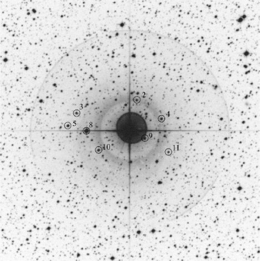
Figure 1.— $\ell$ Car  field with astrometric reference stars marked. Box is 15^′ across.

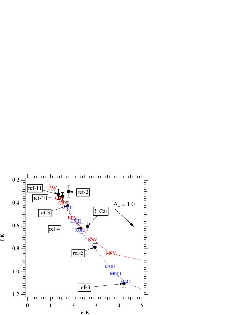
Figure 2.— J-K vs V-K color-color diagram for $\ell$ Car  and reference stars. The dashed line is the locus of dwarf (luminosity class V) stars of various spectral types; the dot-dashed line is for giants (luminosity class III). The reddening vector indicates A_V=1.0 for the plotted color systems. For this low-Galactic latitude field $\langle A_{V}\rangle$ = 0.52 $\pm$ 0.06 magnitude (Table 4).

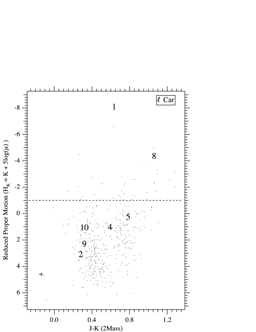
Figure 3.— Reduced proper motion diagram for 430 stars in a $1/3$ degree field centered on $\ell$ Car . Star identifications are shown for $\ell$ Car  (‘1’) and our astrometric reference stars. H_K for these stars is calculated using our final proper motions (Table 7). For a given spectral type giants and sub-giants have more negative H_K values and are redder than dwarfs in J-K. Reference stars ref-4, -5, and -8 are confirmed to be giant stars. The cross in the lower left corner indicates representative errors along each axis.

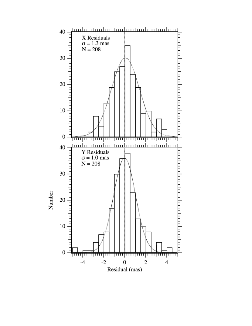
Figure 4.— Histograms of x and y residuals obtained from modeling $\ell$ Car  and astrometric reference stars with equations 4 and 5, constraining D=-B and E=A. Distributions are fit with gaussians whose 1-$\sigma$ dispersions are noted in the plots.

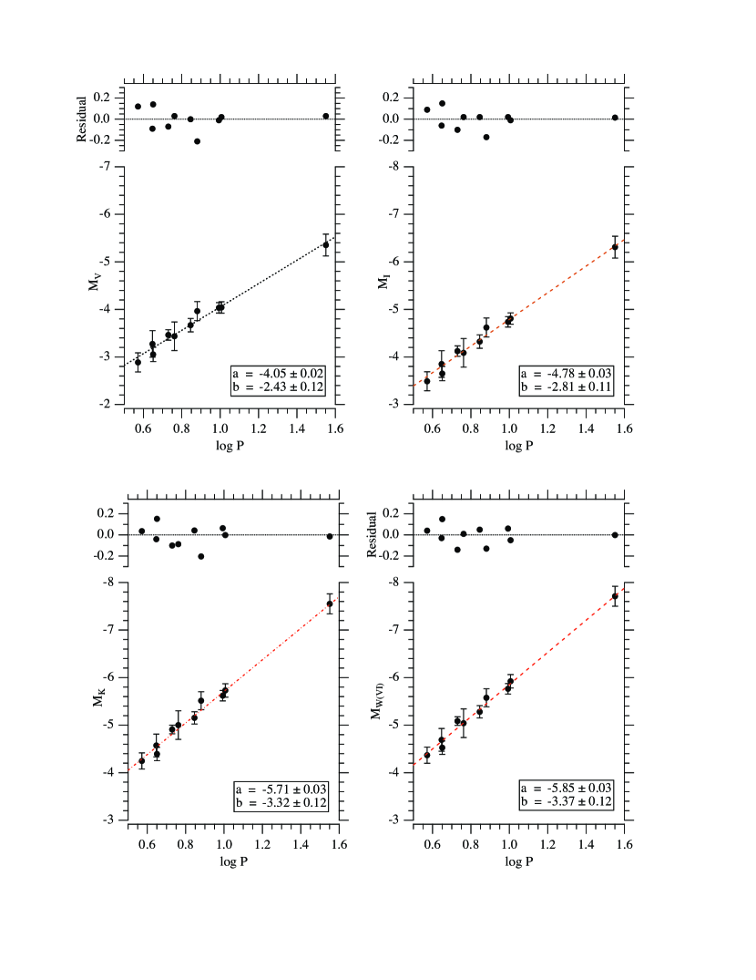
Figure 5.— Period-Luminosity relations for V, I, K, and Wesenheit W_VI, where W_VI = $\langle$V$\rangle$-2.45($\langle$V$\rangle$-$\langle$I$\rangle$). Coefficients are for M $=a+b*(logP-1)$. Errors are $1\sigma$.

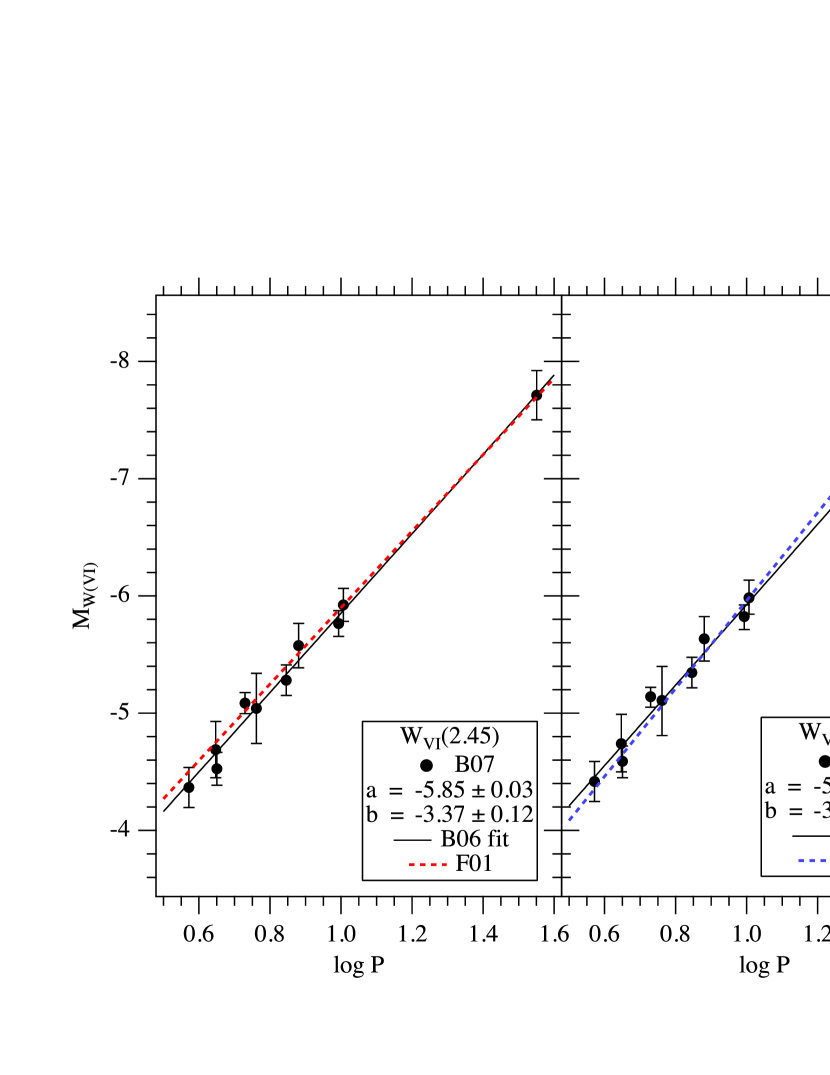
Figure 6.— M_W(VI) Period-Luminosity relations for the present work compared to those adopted by Freedman et al.  [2001] (left) and Sandage et al.  [2004] (right). For the Freedman comparison we use 2.45 as our W_VI color coefficient. For the Sandage comparison we recalculate our W_VI using a 2.52 coefficient. While the Sandage et al. PLR agrees better with the bulk of our Cepheids, the Freedman et al. PLR better matches ours for logP$>$1. Most H₀ Key Project extragalactic Cepheids are long-period. Hence our new PLR has minimal impact on the Freedman et al. H₀ value. If adopted, our PLR would tend to increase the Sandage et al. (2006) H₀ value.

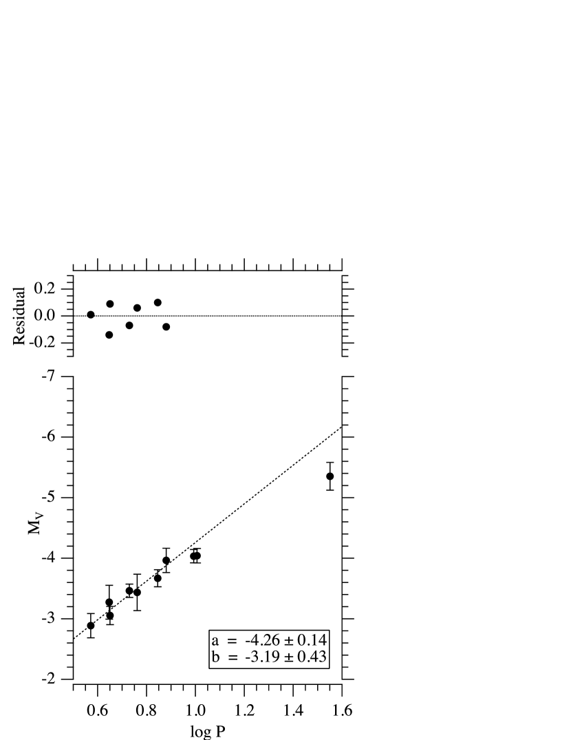
Figure 7.— Period-Luminosity relation for M_V where we fit the seven Cepheids in our sample with logP$<1$. This fit excludes $\ell$ Car , $\zeta$ Gem, and $\beta$ Dor which has logP = 0.9931. Coefficients are for M $=a+b(logP-1.0)$. The slopes differ by $\sim 2\sigma$, comparing the logP $<$ 1 slope against the entire range (Figure 5). Our parallaxes provide only weak evidence for a break at logP = 1.

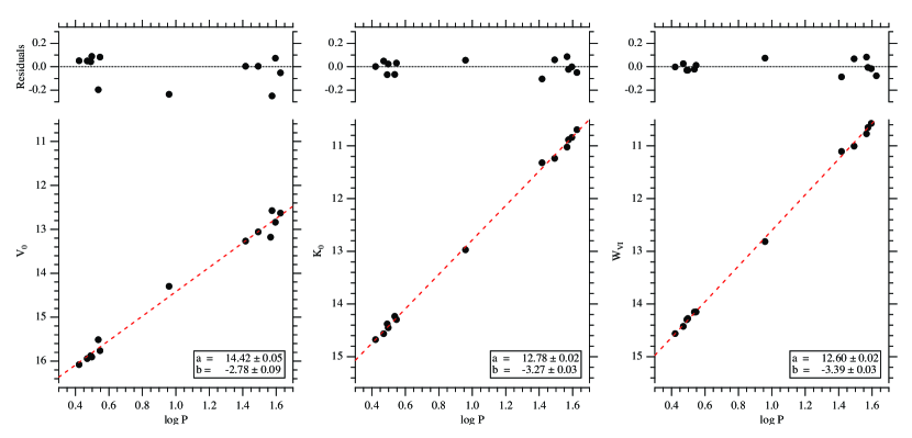
Figure 8.— Period-Luminosity relations for absorption-corrected V, K, and W_VI for 13 LMC Cepheids from Gieren et al.  [2005]. The K-band magnitudes have been transformed to the CIT system. Coefficients are for M $=a+b(logP-1.0)$. The K-band and W_VI slopes are in better agreement with the Galactic Cepheid results than the V-band slope (Figure 5).

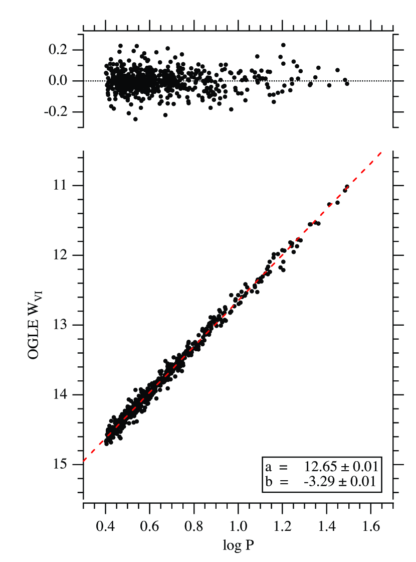
Figure 9.— W_VI Period-Luminosity relation for 581 LMC Cepheids from OGLE. Coefficients are for M $=a+b(logP-1.0)$ and W_VI = $\langle$V$\rangle$-2.45($\langle$V$\rangle$-$\langle$I$\rangle$).

References

- Alcock et al. [1995] Alcock, C. et al. , 1995 AJ, 109, 1653
- Antonello et al. [1990] Antonello, E., Poretti, E., & Reduzzi, L. 1990, A&A, 236, 138
- Barnes et al. [1997] Barnes, T. G., Fernley, J. A., Frueh, M. L., Navas, J. G., Moffett, T. J., & Skillen, I. 1997, PASP, 109, 645
- Barnes et al. [2003] Barnes, T. G., Jefferys, W. H., Berger, J. O., Mueller, P. J., Orr, K., & Rodriguez, R. 2003, ApJ, 592, 539
- Benedict et al. [1998] Benedict, G. F., McArthur, B., Nelan, E., Story, D., Whipple, A. L., Shelus, P. J., Jefferys, W. H., Hemenway, P. D., Franz, O. G., Wasserman, L. H., Duncombe, R. L., van Altena, W., & Fredrick, L. W. 1998, AJ, 116, 429
- Benedict et al. [2002a] Benedict, G. F., McArthur, B. E., Fredrick, L. W., Harrison, T. E., Lee, J., Slesnick, C. L., Rhee, J., Patterson, R. J., Nelan, E., Jefferys, W. H., van Altena, W., Shelus, P. J., Franz, O. G., Wasserman, L. H., Hemenway, P. D., Duncombe, R. L., Story, D., Whipple, A. L., & Bradley 2002a, AJ, 123, 473
- Benedict et al. [2002b] Benedict, G. F., et al. 2002b, AJ, 124, 1695
- Berdnikov et al. [1996] Berdnikov, L. N., Vozyakova, O. V., & Dambis, A. K. 1996, Astronomy Letters, 22, 334
- Berdnikov et al. [2000] Berdnikov, L. N., Dambis, A. K., & Vozyakova, O. V. 2000, A&ASuppl., 143, 211.
- Bessell & Brett [1988] Bessell, M. S. & Brett, J. M. 1988, PASP, 100, 1134
- Caldwell & Coulson [1986] Caldwell, J. A. R., & Coulson, I. M. 1986, MNRAS, 218, 223
- Carpenter [2001] Carpenter, J. M. 2001, AJ, 121, 2851
- Ciardi [2004] Ciardi, D., 2004, private communication
- Cox [2000] Cox, A. N. 2000, Allen’s astrophysical quantities, 4th ed. Publisher: New York: AIP Press, Springer, 2000. Edited by Arthur N. Cox.
- Evans et al. [1990] Evans, N. R., Welch, D. L., Scarfe, C. D., & Teays, T. J. 1990, AJ, 99, 1598
- Evans [1991] Evans, N. R. 1991, ApJ, 372, 597
- Evans [1995] Evans, N. R. 1995, ApJ, 445, 393
- Evans & Massa [2007] Evans, N. R. & Massa, D. 2007, AAS, 209, 151.08
- Feast [1997] Feast, M. W. 1997a, MNRAS, 284, 761
- Feast & Catchpole [1997] Feast, M. W. & Catchpole, R. M. 1997b, MNRAS, 286, L1
- Feast et al. [1998a] Feast, M. W., Pont, F., & Whitelock, P. 1998a, MNRAS, 298, L43
- Feast [1998b] Feast, M. W. 1998b, Mem. Soc. Ast. It. 69, 31
- Feast [1999] Feast, M. W. 1999, PASP, 111, 775
- Feast [2002] Feast, M. W. 2002, MNRAS, 337, 1035
- Fernie, Evans, Beattie, & Seager [1995] Fernie, J. D., Evans, N. R., Beattie, B., & Seager, S. 1995, Information Bulletin on Variable Stars, 4148, 1
- Fitzpatrick et al. [2003] Fitzpatrick, E. L., Ribas, I., Guinan, E. F., Maloney, F. P., & Claret, A. 2003, ApJ, 587, 685
- Freedman et al. [2001] Freedman, W. L., Madore, B. F., Gibson, B. K., Ferrarese, L., Kelson, D. D., Sakai, S., Mould, J. R., Kennicutt, R. C., Jr., Ford, H. C., Graham, J. A.,Huchra, J. P., Hughes, S. M. G., Illingworth, G. D., Macri, L. M., & Stetson, P. B., 2001, ApJ, 553, 47
- Gieren, Barnes, & Moffett [1993] Gieren, W. P., Barnes, T. G., & Moffett, T. J. 1993, ApJ, 418, 135
- Gieren et al. [2005] Gieren, W., Storm, J., Barnes, T. G., Fouqué, P., Pietrzyński, G., & Kienzle, F. 2005, ApJ, 627, 224
- Gould & Morgan [2003] Gould, A. & Morgan, C. W. 2003, ApJ, 585, 1056
- Groenewegen [1999] Groenewegen, M. A. T. 1999, A&ASupp, 139, 245
- Groenewegen & Oudmaijer [2000] Groenewegen, M. A. T. & Oudmaijer, R. D., 2000, A&A, 356, 849
- Groenewegen et al. [2004] Groenewegen, M. A. T., Romaniello, M., Primas, F., & Mottini, M. 2004, A&A, 420, 655
- Hanson [1979] Hanson, R. B. 1979, MNRAS, 186, 875
- Henry [2004] Henry, T. J. 2004, ASP Conf. Ser. 318: Spectroscopically and Spatially Resolving the Components of the Close Binary Stars, 318, 159
- Herrnstein et al. [1999] Herrnstein, J. R., et al. 1999, Nature, 400, 539
- Jefferys et al. [1988] Jefferys, W., Fitzpatrick, J., and McArthur, B. 1988, Celest. Mech. 41, 39.
- Kennicutt et al. [1998] Kennicutt, R. C. et al. 1998, ApJ, 498, 181
- Kervella et al. [2004] Kervella, P., Bersier, D., Mourard, D., Nardetto, N., Fouqué, P., & Coudé du Foresto, V. 2004, A&A, 428, 587
- Kervella [2006] Kervella, P. 2006, Memorie della Societa Astronomica Italiana, 77, 227
- Kienzle et al. [1999] Kienzle, F., Moskalik, P., Bersier, D., & Pont, F. 1999, A&A, 341, 818
- Kiss [1998] Kiss, L. L. 1998, MNRAS, 297, 825
- Lanoix, Paturel, & Garnier [1999] Lanoix, P., Paturel, G., & Garnier, R. 1999, MNRAS, 308, 969
- Leavitt & Pickering [1912] Leavitt, H. S., & Pickering, E. C. 1912, Harvard College Observatory Circular, 173, 1
- Lutz & Kelker [1973] Lutz, T. E. & Kelker, D. H. 1973, PASP, 85, 573
- Macri [2005] Macri, L. M. 2005, ArXiv Astrophysics e-prints, arXiv:astro-ph/0507648
- Macri et al. [2006] Macri, L. M., Stanek, K. Z., Bersier, D., Greenhill, L., & Reid, M. 2006, ApJ, 652, 1133
- Madore & Freedman [1992] Madore, B. F., & Freedman, W. L. 1992, PASP, 104, 362
- Majewski et al. [2000] Majewski, S. R., Ostheimer, J. C., Kunkel, W. E., & Patterson, R. J. 2000, AJ, 120, 2550
- Mathias et al. [2006] Mathias, P., Gillet, D., Fokin, A. B., Nardetto, N., Kervella, P., & Mourard, D. 2006, A&A, 457, 575
- McArthur et al. [2001] McArthur, B. E., Benedict, G. F., Lee, J., van Altena, W. F., Slesnick, C. L., Rhee, J., Patterson, R. J., Fredrick, L. W., Harrison, T. E., Spiesman, W. J., Nelan, E., Duncombe, R. L., Hemenway, P. D., Jefferys, W. H., Shelus, P. J., Franz, O. G., & Wasserman, L. H. 2001, ApJ, 560, 907
- McArthur et al. [2002] McArthur, B., Benedict, G. F., Jefferys, W. H., & Nelan, E. 2002, The 2002 HST Calibration Workshop : Hubble after the Installation of the ACS and the NICMOS Cooling System, Proceedings of a Workshop held at the Space Telescope Science Institute, Baltimore, Maryland, October 17 and 18, 2002. Edited by Santiago Arribas, Anton Koekemoer, and Brad Whitmore. Baltimore, MD: Space Telescope Science Institute, 2002, p.373
- Merand et al. [2005] Merand, A., Kervella, P., Coudé du Foresto, V. et al. 2005, A&A, 438, 9
- Mignard [2005] Mignard, F. 2005, ASP Conf. Ser. 338: Astrometry in the Age of the Next Generation of Large Telescopes, 338, 15
- Moffett & Barnes [1984] Moffett, T.J., & Barnes, T.G. 1984, ApJS, 55, 389
- Nelan et al. [2003] Nelan, E., et al. , 2003 “Fine Guidance Sensor Instrument Handbook,” version 12.0, Baltimore, STScI
- Ngeow et al. [2005] Ngeow, C.-C., Kanbur, S. M., Nikolaev, S., Buonaccorsi, J., Cook, K. H., & Welch, D. L. 2005, MNRAS, 363, 831
- Ngeow [2006] Ngeow, C.-C. 2006, PASP, 118, 349
- Ngeow & Kanbur [2006] Ngeow, C., & Kanbur, S. M. 2006, ApJ, 642, L29
- Nordgren et al. [2002] Nordgren, T. E, Lane, B. F., Hindsley, R. B., & Kervella, P. 2002, AJ, 123, 3380
- Paltoglou & Bell [1994] Paltoglou, G. & Bell, R. A. 1994, MNRAS, 268, 793
- Perryman et al. [1997] Perryman, M. A. C., Lindegren, L., Kovalevsky, J., Hoeg, E., Bastian, U., Bernacca, P. L., Crézé, M., Donati, F., Grenon, M., van Leeuwen, F., van der Marel, H., Mignard, F., Murray, C. A., Le Poole, R. S., Schrijver, H., Turon, C., Arenou, F., Froeschlé, M., & Petersen, C. S. 1997, A&A, 323, L49
- Persson et al. [2004] Persson, S. E., Madore, B. F., Krzemiński, W., Freedman, W. L., Roth, M., & Murphy, D. C. 2004, AJ, 128, 2239
- Petterson et al. [2004] Petterson, O. K. L., Cottrell, P. L., & Albrow, M. D. 2004, MNRAS, 350, 95
- Sachkov [1997] Sachkov, M. E. 1997, Informational Bulletin on Variable Stars, 4522, 1
- Sandage et al. [2004] Sandage, A., Tammann, G. A., & Reindl, B. 2004, A&A, 424, 43
- Sandage et al. [2006] Sandage, A., Tammann, G. A., Saha, A., Reindl, B., Macchetto, F. D., & Panagia, N. 2006, ArXiv Astrophysics e-prints, arXiv:astro-ph0603647
- Savage & Mathis [1979] Savage, B. D. & Mathis, J. S. 1979, ARA&A,17, 73
- Schlegel et al. [1998] Schlegel, D. J., Finkbeiner, D. P., & Davis, M. 1998, ApJ, 500, 525
- Smith [2003] Smith, H. 2003, MNRAS, 338, 891
- Soderblom et al. [2005] Soderblom, D. R., Nelan, E., Benedict, G. F., McArthur, B., Ramirez, I., Spiesman, W., & Jones, B. F. 2005, AJ, 129, 1616
- Standish [1990] Standish, E. M., Jr. 1990, A&A, 233, 252
- Szabados [1989] Szabados, L. 1989, Comm. Konkoly Obs., No. 94
- Szabados [1991] Szabados, L. 1991, Comm. Konkoly Obs., No. 96
- Udalski et al. [1999] Udalski, A., Szymanski, M., Kubiak, M., Pietrzynski, G., Soszynski, I., Wozniak, P., & Zebrun, K. 1999, Acta Astronomica, 49, 201
- Unwin [2005] Unwin, S. C. 2005, American Astronomical Society Meeting Abstracts, 206, #14.03
- van Altena Lee & Hoffleit [1995] van Altena, W. F., Lee, J. T., & Hoffleit, E. D. 1995, Yale Parallax Catalog (4th ed. ; New Haven, CT: Yale Univ. Obs.)(YPC95)
- Yong & Lambert [2003] Yong, D. & Lambert, D. L. 2003, PASP, 115, 796
- Zacharias et al. [2004] Zacharias, N. et al. 2004, AJ, 127, 3043
- Zaritsky et al. [1994] Zaritsky, D., Kennicutt, R. C., Jr., & Huchra, J. P. 1994, ApJ, 420, 87