Seismology of Procyon A: determination of mode frequencies, amplitudes, lifetimes, and granulation noise

The F5 IV-V star Procyon A ($\alpha\!-\!\rm CMi$) was observed in January 2001 by means of the high resolution spectrograph SARG operating with the TNG $3.5\,\rm m$ Italian telescope (Telescopio Nazionale Galileo) at Canary Islands, exploiting the iodine cell technique. The time-series of about 950 spectra carried out during 6 observation nights and a preliminary data analysis were presented in Claudi et al. (2005). These measurements showed a significant excess of power between $0.5$ and $1.5\,\rm mHz$, with $\simeq 1\,\rm m\,s^{-1}$ peak amplitude. Here we present a more detailed analysis of the time-series, based on both radial velocity and line equivalent width analyses. From the power spectrum we found a typical $p$-mode frequency comb-like structure, identified with a good margin of certainty $11$ frequencies in the interval $500-1400\,\rm\mu Hz$ of modes with $l=0,1,2$ and $7\leq n\leq 22$, and determined large and small frequency separations, $\Delta\nu=55.90\pm 0.08\,\mu\rm{Hz}$ and $\delta\nu_{02}=7.1\pm 1.3\,\rm\mu Hz$, respectively. The mean amplitude per mode ($l=0,1$) at peak power results to be $0.45\pm 0.07\,\rm m\,s^{-1}$, twice larger than the solar one, and the mode lifetime $2\pm 0.4\,\rm d$, that indicates a non-coherent, stochastic source of mode excitation. Line equivalent width measurements do not show a significant excess of power in the examined spectral region but allowed us to infer an upper limit to the granulation noise.

1 Introduction

Procyon A ($\alpha\!-\!\rm CMi$, HR 2943, HD61421), hereinafter simply called Procyon, is a F5 IV-V star with $\rm V=0.363$ at a distance of $3.53\,\rm pc$ in a $40\,\rm y$ period visual binary system, the companion being a white dwarf more than $10\,\rm mag$ fainter. By adopting the very accurate parallax measured by HIPPARCOS, $\Pi=285.93\pm 0.88\,\rm mas$, Allende Prieto et al. (2002) derived a mass of $1.42\pm 0.06\,\rm M_{\odot}$, a radius of $2.071\pm 0.02\,\rm R_{\odot}$, and a gravity $\log g=3.96\pm 0.02$.

Procyon, owing to its proximity and brightness, has already attracted attention of stellar seismologists (Brown et al. 1991; Guenther & Demarque 1993; Barban et al. 1999; Chaboyer et al. 1999; Martić et al. 1999, 2004; Eggenberger et al. 2004), causing an intense debate among the scientists. The excess of power in the range $0.5-1.5\,\rm mHz$ found by Bouchy et al. (2004), Martić et al. (2004), Eggenberger et al. (2004), and Claudi et al. (2005), hereinafter referred as Paper I, seems to have a stellar origin and is consistent with a $p$-mode comb-like pattern.

However, data from the Canadian MOST satellite (Matthews et al. 2004) show no significant power excess in the same spectral region. To this regard Bedding et al. (2005) suggested that the most likely explanation for the null detection could be a dominating non-stellar noise source in the MOST data, though Régulo & Roca Cortés (2005) claimed for the presence of a signal in these data.

In Paper I we presented high precision radial velocity measurements carried out during 6 observation nights by means of the high resolution spectrograph SARG operating with TNG $3.5\,\rm m$ Italian telescope (Telescopio Nazionale Galileo) at Canary Islands. The data showed an excess of power between $0.5-1.5\,\rm mHz$ with a large separation of about $56\pm 2\,\mu\rm Hz$, in agreement with previous measurements of Mosser et al. (1998), Barban et al. (1999), Martić et al. (1999, 2004) and Eggenberger et al. (2004), who found values in the range $53-56\,\rm\mu Hz$. Here we deal with an improvement of the preliminary analysis presented in Paper I concerning an accurate time-series analysis of both radial velocities and line equivalent width measurements, from which mode frequencies, amplitudes and lifetimes are determined and constraints on stellar granulation noise are deduced.

2 Observations

SARG is a high resolution cross dispersed echelle spectrograph (Gratton et al. 2001) which operates in both single object and long slit (up to $26^{\prime\prime}$) observing modes and covers a spectral wavelength range from $370\,\rm nm$ up to about $1000\,\rm nm$, with a resolution ranging from $R=29,000$ up to $R=164,000$. Our spectra were obtained at $R=144,000$ in the wavelength range between $462-792\,\rm nm$. The calibration iodine cell works only in the blue part of the spectrum ($462-620\,\rm nm$) that has been used for measuring Doppler shifts. The red part of the echelle spectrum of Procyon has been used for measuring line equivalent widths of absorption lines sensitive to temperature. During the observing period we collected about 950 high signal-to-noise ratio (S/N) spectra with a mean exposure time of about $10\,\rm s$ (see Paper I for more details). The red part spectrum has been calibrated in wavelength by using a Th-Ar lamp. The analysis of both the blue and red parts of the spectrum was performed by using the IRAF package facilities.

3 Radial velocity measurements and analysis

Radial velocities have been determined by means of the AUSTRAL code (Endl et al. 2000) which models instrumental profile, stellar and iodine cell spectra in order to measure Doppler shifts (see also Paper I). This code also provides an estimate of the uncertainty in the velocity measurements, $\sigma_{i}$. These values have been derived from the scatter of velocities measured from many ($\simeq 100$), small ($\simeq 2\,$Å) segments of the echelle spectrum. In order to perform a weighted Fourier analysis of the data, we firstly verified that these $\sigma_{i}$ values reflected the noise properties of the velocity measurements, following Butler et al. (2004) approach. The high frequency noise in the power spectrum (PS) well beyond the stellar signal, reflects the properties of the noise in the data, and since we do expect that the oscillation signal is the dominant cause of variations in the velocity time series, we need to remove it before to analyze the noise. We do that iteratively by finding the strongest peak in the PS of the velocity time-series and subtracting the corresponding sinusoid from the time-series. This procedure is carried out for the strongest peaks in the oscillation spectrum in the frequency range $0-2\,\rm mHz$, until the spectral leakage into high frequencies from the remaning power is negligible. Thus we have a time series of residual velocities, $r_{i}$, that reflects the noise properties of the measurements. We then analyze the ratio $r_{i}/\sigma_{i}$, which is expected to be Gaussian-distributed, so that the outliers correspond to the suspected data points. The cumulative histogram of $|r_{i}/\sigma_{i}|$ is shown in the upper panel of Fig. 1.

Figure 1: Upper panel: cumulative histograms of $|r_{i}/\sigma_{i}|$ for SARG data. The diamonds show the observed data, and the solid curve shows the result expected for a Gaussian-distributed noise. Lower panel: ratio of the observed to the expected histograms, indicating the fraction of “good” data points.

The solid curve shows the cumulative histogram for the best-fit Gaussian distribution. A significant excess of outliers is evident for $|r_{i}/\sigma_{i}|\geq 2$. The lower panel of Fig. 1 shows the ratio of the values of the observed points to the corresponding ones of the Gaussian curve, i.e. the fraction $f$ of data points that could be considered as “good” observations, namely those which are close to the unity. The quantities $w_{i}=1/(\sigma_{i}^{2}f)$ have been adopted as weights in the computation of the weighted PS shown in Fig. 2, where the most prominent peak has an amplitude of $\simeq 1\,\rm m\,s^{-1}$.

Figure 2: The power spectrum of the weighted data. An excess of power around $1\,\rm mHz$ is evident. The inset shows the power spectrum of the window function for a sine-wave signal of amplitude $1\,\rm m\,s^{-1}$, sampled in the same way as the observations. The power units are the same as those of the main figure.

3.1 Search for a comb-like pattern

In solar-like stars, $p$-mode oscillations of low harmonic degree, $l$, and high radial order, $n$, are expected to produce in the PS a characteristic comb-like structure with mode frequencies $\nu_{n,l}$ reasonably well approximated by the Tassoul’s simplified asymptotic relationship (Tassoul 1980):

$$\nu_{n,l}\simeq\Delta\nu(n+{l}/{2}+\varepsilon)-l(l+1)\delta\nu_{02}/6$$ (1)

where $\Delta\nu=<\nu_{n,l}-\nu_{n-1,l}>$ and $\delta\nu_{02}=<\nu_{n,0}-\nu_{n-1,2}>$ are the average large frequency separation and small frequency separation for $l=0,2$, respectively, and $\varepsilon$ is a constant of the order of unity, sensitive to the sound speed near the surface layers of the star. $\Delta\nu$ reflects the average stellar density, while $\delta\nu_{02}$ is largely determined by the conditions in the core of the star and reflects its evolutionary state. In order to estimate the large frequency separation $\Delta\nu$ in the region of the excess of power detected in the PS, we applied the comb-response method, that is a generalization of the PS of a PS and consequently allows us to search for any regularity in a spectral pattern. The comb-response function, CR($\Delta\nu$), is defined by Kjeldsen et al. (1995) as the following products of PS calculated for a series of trial values $\Delta\nu$:

$$\rm CR(\Delta\nu)= \rm PS(\xi_{-1/2})PS(\xi_{+1/2})PS(\xi_{-1})PS(\xi_{+1})\times$$ (2)

$$\left[\rm PS(\xi_{-3/2})PS(\xi_{+3/2})PS(\xi_{-2})PS(\xi_{+2})\right]^{1/2}$$

where $\xi_{\pm k}=\nu_{\rm max}\pm k\Delta\nu$, with $\nu_{\rm max}$ the frequency of the strongest peak in the PS. A peak in the CR at a particular spacing $\Delta\nu$ indicates the presence of a regular series of peaks in the PS, centred at the central frequency $\nu_{\rm max}$ – tentatively assumed to be an oscillation mode – and having a spacing $\Delta\nu/2$. In order to select the central frequencies $\nu$’s for the CR analysis we evaluated the white noise in the PS between $2.5-3.0\,\rm mHz$ and adopted as $\nu_{\rm max}$’s the frequencies of the peaks in the PS between $0.5-1.5\,\rm mHz$ with $\rm S/N>4$. For each central frequency $\nu_{\rm max}$ we searched for the maximum CR in the range $20\leq\Delta\nu\leq 80\,\rm\mu Hz$. Figure 3 reports the $\Delta\nu$’s determined from the CR analysis, that gives a mean value $\Delta\nu=55.7\pm 1.4\,\rm\mu Hz$, where the error is the standard deviation, and Fig. 4 the cumulative CR function computed as the sum of all the individual CR functions referring to each central frequency $\nu_{\rm max}$, that gives $\Delta\nu=56\pm 1\,\rm\mu Hz$, where the error is the FWHM of the peak.

Figure 3: The first-order spacing calculated over several frequency ranges, as determined from the comb-response analysis. The line shows the mean value of $55.7\,\rm\mu Hz$, with a standard error of $\pm 1.4\,\rm\mu Hz$.

Figure 4: The cumulative comb-response obtained as the sum of the individual comb-responses for each central frequency $\nu_{0}$. The peak is centred at $\Delta\nu=56\pm 1\,\rm\mu Hz$. The error is the FWHM of the peak.

3.2 Oscillation frequencies and mode amplitude

By assuming the $56\,\rm\mu Hz$ regularity as genuine, we attempted to identify the oscillation frequencies directly from the PS. In order to extract the frequencies we used the following procedure (“standard” extraction): i) we found the largest peak, in the frequency range $0.5-1.5\,\rm mHz$, then subtracted the corresponding sine-wave function from the time-series, finally recomputed the PS; ii) we repeated such a procedure for the new largest peak in the same range of frequency, the procedure being stopped when there were no peaks with amplitude larger than $0.29\,\rm m^{2}\,s^{-2}$, namely larger than $3\sigma$, where $\sigma$ is the white noise evaluated in the PS between $2.5-3\,\rm mHz$. The extracted frequencies are plotted in the echelle diagram shown in Fig. 5.

Figure 5: The echelle diagram as derived from the “standard” extraction of frequencies.

Owing to single site observations, we need to take into account the daily alias of $11.57\,\rm\mu Hz$ (see the spectral window in Fig. 2) in order to identify the modes in the echelle diagram; in fact, we cannot know a priori whether or not the frequencies, selected by the iterative procedure described above, are the correct ones or just aliases. Therefore, instead of shifting the frequencies by the daily alias, that, for each shift, might lead to an arbitrary identification of the modes, we prefer to use a procedure (“modified” extraction) which relies on two assumptions only: i) the largest peak in the range of interest is a true pulsation mode; ii) the large separation value is $56\,\rm\mu Hz$. We operated in the same way as in the point i) of the “standard” extraction, then defined a new searching spectral region centred at a distance of $56\,\rm\mu Hz$ from the first component, the extension of which was $2\,\rm\mu Hz$, a suitable frequency span related to spectral resolution. If this region contained a peak with an amplitude larger than $3\sigma$, we identified this peak as the second component to be cleaned, and recomputed the PS. This process was repeated, shifting frequency back and forward by multiples of $56\,\rm\mu Hz$, and once the whole region of interest had been covered, the remaining largest peak was identified and the process restarted with a new set of searching regions separated again by $56\,\rm\mu Hz$, the procedure being stopped when all remaining peaks were below the $3\sigma$ threshold. This is the same procedure as that used by Kjeldsen et al. (1995) for $\eta\,\rm Boo$, that allows to determine the mode frequencies except for the daily alias that could cause a shift of $\pm 11.57\,\rm\mu Hz$. The frequencies extracted with this procedure are shown in Table 1 and the related echelle diagram in Fig. 6.

Table 1: Prominent peaks in the power spectrum of Procyon identified as mode oscillation frequencies (in $\rm\mu Hz$) in terms of $n$ and $l$. The values of $n$ are deduced from the fit to the asymptotic relationship (1). The frequency indicated in parenthesis was excluded from the fit because of its large deviation from the asymtotic relationship, though the related peak in the power spectrum is a high S/N one.

$n$	$l=0$	$l=1$	$l=2$
7		524.5
9	608.4
11			770.0
12	778.7	(808.6)
13	834.3
18	1114.2	1138.8
20	1224.2	1252.0
22	1335.4

Figure 6: The echelle diagram as derived from the “modified” extraction of frequencies.

The large and small frequency separations, and the constant $\varepsilon$ have been determined by means of a least square best fit of frequencies with the asymptotic relationship (1), obtaining: $\Delta\nu=55.90\pm 0.08\,\rm\mu Hz$, $\delta\nu_{02}=7.1\pm 1.3\,\rm\mu Hz$, $\varepsilon=1.913\pm 0.025$, with a rms scatter per mode of $1.23\,\rm\mu Hz$. In Table 1 we also give a possible mode with $l=1$ and $n=12$ at $808.6\,\rm\mu Hz$, however this mode was excluded from the calculation of the fit because of its large deviation from the asymptotic relation, though the related peak in the power spectrum is a high S/N one. Once determined $\Delta\nu$, it is possible to construct a folded spectrum where the power in the PS is folded at the large separation, by using the frequency modulo of $55.90\,\rm\mu Hz$. The result is shown in Fig. 7 where the mean power as a function of frequency modulo is plotted, and the positions of modes with $l=0,1,2$ are given together with the positions of the daily side-bands, from which the detection of a $p$-mode structure in Procyon is evident.

Figure 7: The mean power folded at the large separation frequency as a function of frequency modulo of $55.90\,\rm\mu Hz$. The positions of the modes with $l=0,1,2$ are indicated together with the positions of the daily side-bands.

The amplitude of individual modes can be estimated from the power concentrated in the PS, on assuming that, owing to the full disc observations, only $l=0,1,2,3$ modes are detected. It is then possible to estimate the amplitude per mode necessary for producing the observed power level. Following the procedure described in Kjeldsen et al. (2005) we found a mean amplitude of the $p$-mode peak power, for the modes with $l=0,1$ in the frequency interval $0.6-1.4\,\rm mHz$, of $0.45\pm 0.07\,\rm m\,s^{-1}$, that is a value twice larger than the solar one and in very good agreement with the amplitudes estimated by Brown et al. (1991). Our velocity amplitude can be transformed in intensity amplitude by using the Kjeldsen & Bedding (1995) method, and obtaining, at $5500\,\AA$, the value of $7.3\pm 1.1\,\rm ppm$ per mode ($l=0,1$) in good agreement with the WIRE (Bruntt et al. 2005) and upper limit MOST (Matthews et al. 2004) measurements. The results are summarized in Fig. 8 where the velocity amplitude per mode is shown as a function of frequency together with the intensity scale and the equispaced positions of $l=0$ modes as derived from the relationship (1) in which the determined values of $\Delta\nu$ and $\varepsilon$ were inserted.

Figure 8: Velocity amplitude per mode ($l=0,1$) as a function of frequency. The horizontal line at $0.45\,\rm m\,s^{-1}$ represents the mean amplitude of the $p$-mode peak power in the frequency interval $0.6-1.4\,\rm mHz$. The scale of intensity is also given together with the positions of $l=0$ modes, as derived from asymptotic relationship (1).

In Fig. 8 a dip at $1\,\rm mHz$ is clearly visible, that is a confirmation of a previously reported result of Bedding & Kjeldsen (2006), and whose presence is probably related to the damping rate of the modes (Houdek et al. 1999).

3.3 Comparison with other frequency determinations

Our results are directly comparable with those of Eggenberger et al. (2004), as given in their Table 3, where the identified frequencies are tabulated. We may also make a comparison with the raw extracted frequencies given by Eggenberger et al. (2004) in their Table 2. We are not able to make a direct comparison with the results by Martić et al. (2004), since they only provide a list of identified mode frequencies that depend on the fitting to theoretical models.

In order to perform the comparison with Eggenberger et al. (2004) we apply the same least square best fit we applied to our frequency data to those of Eggenberger et al. (2004) and derive the parameters of the asymptotic relationship which result to be: $\delta\nu_{02}=4.9\,\rm\mu Hz$, $\varepsilon=1.537$. In this procedure the value of $\Delta\nu$ has been taken fixed to the value given by Eggenberger et al. (2004), $\Delta\nu=55.5\,\rm\mu Hz$. If one calculate the frequencies corresponding to the two asymptotic solutions, the one in the present paper and the one we obtain by fitting to the Eggenberger et al. (2004) data, we find that most of the calculated frequencies, for $l=0,1$, agree within $3\,\rm\mu Hz$. We find that $l=0$, $n=9-24$ modes from the Eggenberger et al. (2004) asymptotic relation correspond to $l=1$, $n=8-23$ modes from the asymptotic relation in the present study. We also find that $l=1$, $n=7-22$ (Eggenberger et al. (2004)) modes correspond to $l=0$, $n=7-22$ modes identified by us. We conclude that we and Eggenberger et al. (2004) are detecting signal from the same underlying p-modes. If we look at all the raw extracted frequencies given by Eggenberger et al. (2004) in their Table 2, it appears of striking importance that most of those frequencies may be identified by using the asymptotic solution deduced from the present study. In table 2 we compare the Eggenberger et al. (2004) raw frequencies with the asymptotic relation from the present study ($\Delta\nu=55.90\,\rm\mu Hz$, $\delta\nu_{02}=7.1\,\rm\mu Hz$, $\varepsilon=1.913$).

Table 2: Comparison between the Eggenberger et al. (2004) extracted raw frequencies (in $\rm\mu Hz$) and the asymptotic relation from the present study ($\Delta\nu=55.90\,\rm\mu Hz$, $\delta\nu_{02}=7.1\,\rm\mu Hz$, $\varepsilon=1.913$).

Raw frq.	Correction	Fit			This study
$\nu$		$\nu$	$l$	$n$
630.8					Noise?
651.5	+ 11.6 = 663.1	665.9	0	10
662.7		665.9	0	10
683.5	+ 11.6 = 695.1	691.5	1	10	?
720.6		721.8	0	11
791.8	- 11.6 = 780.2	777.7	0	12	778.7
797.9	(809.5?)	803.3	1	12	808.6?
799.7	(811.3?)	803.3	1	12	808.6?
828.5		826.5	2	12
835.4		833.6	0	13	834.3
856.2		859.2	1	13
859.8		859.2	1	13
911.4		915.1	1	14	?
929.2	+ 11.6 = 940.8	938.3	2	14
1009.7	- 11.6 = 998.1	1001.3	0	16
1027.1		1026.9	1	16
1123.3	- 11.6 = 1111.7	1113.1	0	18	1114.2
1131.1					Noise?
1137.0		1138.7	1	18	1138.8
1186.0	+ 11.6 = 1197.5	1194.6	1	19
1192.4		1194.6	1	19
1234.8	- 11.6 = 1223.2	1124.9	0	20	1224.2
1251.8		1250.5	1	20	1252.0
1265.6	+ 11.6 = 1277.2	1273.7	2	20
1337.2		1336.7	0	22	1335.4
1439.0		1141.4	2	23
1559.5		1560.3	0	26

It is interesting to note that 8, out of 11, frequencies determined by us match well, within a few $\rm\mu Hz$, those listed in the Table 2 of Eggenberger et al. (2004), but with a different mode identification. Therefore we detected signals from the same frequencies as Eggenberger et al. (2004), but extracted the $p$-mode structure in a slightly different way, reaching two different solutions, and therefore identifications, for the extracted frequencies.

If we use our solution, $\Delta\nu=55.90\,\rm\mu Hz$, $\delta\nu_{02}=7.1\,\rm\mu Hz$, $\varepsilon=1.913$, to verify to which extent it matches the Eggenberger et al. (2004) frequencies we find that 16 frequencies match our solution, 5 need a shift of $+11.6\,\rm\mu Hz$, 4 need a shift of $-11.6\,\rm\mu Hz$, and only 2 do not match the solution. Otherwise, if we use the Eggenberger et al. (2004) solution, $\Delta\nu=55.50\,\rm\mu Hz$, $\delta\nu_{02}=4.9\,\rm\mu Hz$, $\varepsilon=1.537$, we find that 12 frequencies match this solution, 8 need a shift of $+11.6\,\rm\mu Hz$, 3 need a shift of $-11.6\,\rm\mu Hz$, and 4 do not match the solution. This means that the frequencies detected by Eggenberger et al. (2004) provide a slightly better fit to our solution than to their solution.

This statement is supported by the fact that if we only look at those 12 frequencies that fit, without shift, the Eggenberger et al. (2004) asymptotic relationship and compare them with the Eggenberger et al. (2004) 16 raw frequencies that fit the solution found in the present study, we see that the scatter for the 16 frequencies is about 10% lower when we use our asymptotic relation. Moreover, Eggenberger et al. (2004) identify the 50% of those 12 frequencies that fit its relation as $l=2$ modes, while the $l=1$ modes should show instead the highest amplitude.

However, since the two solutions provide basically the same frequencies, one should of course be cautious in claiming that one solution is far better than the other one.

3.4 Mode lifetimes

Solar-like $p$-mode oscillations in Procyon are presumably excited stochastically by the action of the surface convection (Houdek et al. 1999) as in the case of the Sun’s oscillations. Therefore it is interesting to give an estimate of the lifetime of modes for verifying the excitation mechanism that in turn determines their observed spectral width and amplitude. A coherent, over-stable, long-lived pulsation mode would concentrate all its power in a small frequency bin, whilst a stochastically, short-lived excited mode would spread its power over a larger frequency interval. In the case of the Sun the mode lifetime, at the peak amplitude of $3\,\rm mHz$, is about $3\pm 1\,\rm d$, as estimated by fitting a model to the power distribution for each mode in the PS (Chaplin et al. 1997). The Chaplin et al. (1997) technique requires observations for a significantly longer time than the mode lifetime, that is not necessarily consistent with our observing period of 6 nights.

The method we use in the present analysis is based on the frequency scatter per identified mode (Bedding et al. 2004; Kjeldsen et al. 2005), as calculated in Section 3.2. We ran 8400 individual simulations in order to determine the rms scatter of the detected frequencies as a function of the mode lifetime, by using the De Ridder et al. (2006) simulator, and neglecting rotational splittings both because Procyon is a slow rotator and the majority of modes used are radial. The simulations contain the mode correct amplitude, noise level, and number of detected modes out of the total number of modes contained in the $p$-mode spectrum, as determined from the asymptotic relationship (1) in the observed frequency interval. The fit represents a model that contains two components: the frequency spread, that is essentially the width of the Lorentzian profile, and the scatter of coherent oscillations, that corresponds to an infinite mode lifetime. The results are reported in Fig. 9 where the rms scatter of the $10$ considered frequencies, out of the $11$ identified (see Section 3.2), is plotted vs. mode lifetime. Since the mode frequency scatter determined in Section 3.2 results to be $1.23\,\rm\mu Hz$, it is easily seen from Fig. 9 that the corresponding lifetime is $2.0\pm 0.4\,\rm d$. The observed frequency scatter in Procyon is sensibly larger than that consistent with coherent oscillations, ruling out this possibility, and the related mode lifetimes appear to be slightly shorter than those observed in the Sun, where the oscillations are excited by the surface turbulent convection. The present data strongly indicate that oscillations in Procyon are not coherent, but damped and re-excited by a mechanism similar to that operating in the Sun, as expected.

Figure 9: The rms scatter of the 10 identified frequencies as a function of mode lifetime obtained by several thousand simulations. The intersection of the horizontal line of the observed scatter with the solid curve obtained by simulations indicates that the mode lifetime is $1.97^{+0.43}_{-0.35}\,\rm d$. The horizontal line of coherent oscillation scatter, corresponding to an infinite mode lifetime, is also indicated. The frequency spread reflects essentially the width of the Lorentzian profile.

The results of the previous method for determining the mode lifetimes are corroborated by a different analysis we performed, based on the amplitude of the highest peaks in the PS, with the idea that also the amplitude of modes are affected by their lifetimes, in the sense that when the peak amplitude is smaller the mode lifetime is shorter, whilst when it is larger the mode lifetime is longer. However, since there is not a simple relationship between amplitude and lifetime, we used a data simulation, based on several thousand runs, that allows a direct comparison between the observed properties of the time-series and the properties of the oscillation modes in order to establish a calibrated relationship between the peak height and the mode lifetime (De Ridder et al. 2006). With respect to the previous one, this method has the advantage of being independent of mode identification but the disadvantage of being less accurate. The result is reported in Fig. 10, where we show the amplitude, with $1\,\sigma$ error bars, of the 6 largest amplitude detected modes with $l=0,1,2$ as a function of the mode lifetime.

Figure 10: The amplitude of the 6 largest amplitude detected modes, for $l=0,1,2$ as a function of the mode lifetime. The bars indicate the $1\,\sigma$ error.

In Fig. 10 the intersection of the horizontal line corresponding to that of the observed mode of largest amplitude (see Fig. 2) with the simulated data gives an average mode lifetime $\simeq 2\,\rm d$, in good agreement with the frequency scatter method but with a much larger uncertainty. It is interesting to note the expected trend of mode amplitudes as a function of their lifetimes.

The effects of frequency scatter and mode amplitude on mode lifetime is evident in Figs. 11 and 12, where simulations concerning $10\,\rm d$ continuous observation campaigns are reported for mode lifetimes of $2\,\rm d$ and $0.5\,\rm d$ respectively. In the above quoted two figures the upper panel shows the complete PS, while the lower one an enlarged portion of it from $0.8\,\rm mHz$ to $1.0\,\rm mHz$. From our simulations it is clearly seen that the frequencies of long-living modes are much better defined, or less scattered, and have larger amplitudes than those of short-living modes.

Figure 11: Simulated Procyon $p$-mode power spectrum obtained by using the De Ridder et al. (2006) simulator not including noise and rotational splittings. The length of the time-series is $10\,\rm d$ and the mode lifetime is $2\,\rm d$.

Figure 12: The same simulation as that of Fig. 11, but for a mode lifetime of $0.5\,\rm d$. Note that the frequency spreads are larger and peak amplitudes are smaller than those of the modes seen in Fig. 11.

4 Line equivalent width measurements and analysis

As already mentioned, the red part of the echelle spectrum of Procyon is insensitive to the iodine cell calibration and therefore the search for stellar pulsations can be performed only by means of measurements of line equivalent widths (EW). The presence of telluric lines and limited number of strong lines sensitive to temperature (e.g. $\rm H_{\alpha}$ is located at the border of spectral orders and is therefore useless for accurate EW measurements) restricted our analysis to the spectral lines reported in Table 3.

Table 3: Spectral line wavelengths used for EW measurements.

Wavelength (Å)	Spectral lines
6393.4	Fe I
6436.7	Ca I
6462.4	Ca I / Fe I
6546.0	Fe I
6574.9	Fe I
6592.7	Fe I
6643.4	Ni I
6677.8	Fe I
6717.5	Ca I

4.1 Power spectrum

Since the expected variations in the EW induced by the stellar pulsations are of the order of a few ppm, we adopted an accurate approach for the measurement of the EW, following Kjeldsen et al. (1995). Instead of fitting the line profile for determining the EW, we computed the flux in three artificial filters, analogously to Strömgren $\rm H_{\beta}$ photometry. The first filter was centred on the considered line at the wavelength $\lambda_{0}$, with a band-width $\Delta\lambda_{0}$, and the other two on the near continuum with respect to the line at $\lambda_{0}$, one placed on the red region at $\lambda_{\rm r}$, with band-width $\Delta\lambda_{\rm r}$, and the other on the blue one at $\lambda_{\rm b}$, with a band-width $\Delta\lambda_{\rm b}$. We then computed the EW, or more precisely the line-index, in terms of the radiation flux measured in the selected filters ${\cal F}(\Delta\lambda)$:

$$\rm EW=\left[\frac{{\cal F}(\Delta\lambda_{0})}{\Delta\lambda_{0}}\right]\cdot\left[\frac{\Delta\lambda_{\rm r}+\Delta\lambda_{\rm b}}{{\cal F}(\Delta\lambda_{\rm r})+{\cal F}(\Delta\lambda_{\rm b})}\right]$$ (3)

for two different central filter widths, $\Delta\lambda^{1}_{0}$ and $\Delta\lambda^{2}_{0}$, in order to obtain two values for the EW, $\rm EW_{1}$ and $\rm EW_{2}$, from which the quantity ${\rm EW_{\rm best}}={\rm EW}_{1}^{m+1}/{\rm EW}_{2}^{m}$ can be constructed. The aim of this procedure is to construct a quantity that is less sensitive to the continuum fluctuations, determining $m$ so as to minimize the scatter of the measurements in a similar way as described for the radial velocity analysis. The procedure was repeated for all the lines reported in Table 3, and then, in order to improve the S/N, we combined all the $\rm EW_{\rm best}$’s obtained for the examined lines, assuming for them the same sensitivity to temperature changes, and derived a weighted mean value. In Figs. 13 and 14 we show the time-series and the weighted PS of the $\rm EW_{\rm best}$, respectively. The weights adopted are $w_{i}=1/{\sigma_{i}^{2}}$, where the $\sigma_{i}$’s are the standard deviations of the data.

Figure 13: Time series of EW measurements as derived from the combination of all the lines reported in Table 3.

Figure 14: The weighted power spectrum $\rm EW_{\rm best}-<\rm EW_{\rm best}>$ derived from the combination of the measurements of all the lines of Table 3. There is no excess of power in the range $0.5-1.5\,\rm mHz$, but the background power in the range $0.2-0.7\,\rm mHz$ could be a signature of stellar granulation.

4.2 Granulation noise

The combined power spectra do not show evidence of power excess in the range $0.5-1.5\,\rm mHz$, as is clear from Fig. 14. However, at low frequencies, some concentration of power, similar to the background power reported by Kjeldsen et al. (1999) for $\alpha\,\rm Cen\,A$, and attributed to stellar granulation, is apparent. Analogously to Kjeldsen et al. (1999), here we attempt to give an estimate of the amount of power related to Procyon granulation. In this procedure we optimize the S/N in the PS by computing the weighted means of the measurements, by using weights that minimize the mean noise for each line in the interval $0.2-0.7\,\rm mHz$, and then rescale the weights for each line in such a way that the weights, $w_{i}$, satisfy the relationship $\sum w_{i}=1/\cal A$, where $\cal A$ is the mean of the peak amplitudes in the range $0.2-0.7\,\rm mHz$.

In order to evaluate the power generated by the granulation of the star in the PS of the EW’s and make a comparison with data obtained with different methods we need to define a quantity independent of the temporal length of the data, that is obtained by computing the power density spectrum (PDS), a measure of the power per frequency resolution element that is therefore independent of the length and sampling of the time-series:

$$\rm PDS(\nu)={\rm A^{2}(\nu)}\left[{\int_{0}^{\nu}\rm N(\nu)W^{2}(\nu)d\nu}\right]^{-1}$$ (4)

where $\rm A(\nu)$ is the amplitude (in ppm) in the PS, $\rm W(\nu)$ the window function, and $\rm N(\nu)$ the Nyquist frequency. The result of our analysis is shown in Fig. 15, where the dashed line (this project) indicates the smoothed power density spectrum of Procyon granulation noise, and background the PDS of the PS shown in Fig. 14.

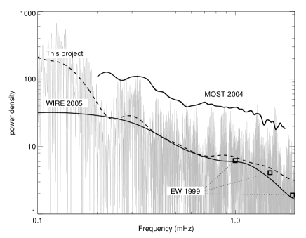
Figure 15: Smoothed power density spectra (PDS) of Procyon granulation noise as obtained from SARG (dashed line, this project) and AAT/ESO [EW 1999, squares, (Kjeldsen et al. 1999)] spectroscopy, and MOST (Matthews et al. 2004) and WIRE (Bruntt et al. 2005) space photometry (continuous lines). On background the PDS derived from the PS of Fig. 14 is shown. Power density is expressed in $\rm ppm^{2}\,\mu Hz^{-1}$.

4.3 Comparison with other granulation noise determinations

The literature reports three previous claims of granulation noise power detection in Procyon. The first is by Kjeldsen et al. (1999), who found a granulation noise slightly above the solar level in the frequency interval $1-2\,\rm mHz$, by using the Balmer EW’s. These determinations are shown in Fig. 15 as squares (EW 1999). The other two claims, instead of spectroscopic, concern space photometric measurements carried out by the satellites MOST (Matthews et al. 2004), operating in the bandwidth $3700-7000\,\AA$, and WIRE (Bruntt et al. 2005), operating with the white light star tracker.

While our measurements are directly comparable with the spectroscopic ones of Kjeldsen et al. (1999), in order to compare them with the photometric ones, we need to pass from intensities, $I$, to temperatures, $T$, and from the latter to EW’s. This is accomplished by using appropriate sensitivity indices; for intensity we used $\partial\ln I/\partial\ln T=4.5$ (Kjeldsen & Bedding 1995), and for EW, $\partial\ln\rm(EW)/\partial\ln T=-7.8$, as deduced from the analysis of Bedding et al. (1996) for Fe I lines at $T=6500\,\rm K$. The results are shown in Fig. 15, where MOST and WIRE PDF curves are plotted together with Kjeldsen et al. (1999) data and our curve.

It appears that, while WIRE and our distribution of power are mutually consistent, at least in the frequency interval $0.2-2\,\rm mHz$, and corroborated by the few data of Kjeldsen et al. (1999), MOST shows a power density level higher by a factor of four or more. Uncertainties in sensitivity index calibration of $I$ and EW with respect to $T$ may lead to some discrepancies, but not so large to explain such a significant disagreement between MOST and other data. In order to render the MOST data comparable with ours, it should be $\mid\partial\ln\rm(EW)/\partial\ln T\mid\;<4.5$ and $\partial\ln I/\partial\ln T>4.5$. This is unlikely because the value of $\partial\ln\rm(EW))/\partial\ln T$ adopted here has been derived by observations of the same lines we use here at the same temperature of Procyon (Bedding et al. 1996) and a value of $\partial\ln I/\partial\ln T>4.5$ is in disagreement with the models of Bedding et al. (1996). This seems to imply that MOST did not detect granulation noise, probably because of some instrumental or stellar spurious signal as suggested by Bruntt et al. (2005).

Differently from the first spectroscopic determinations of Kjeldsen et al. (1999) relative to a few points in the high frequency side of the granulation noise PDS, our EW determinations constitute the first spectroscopic measurements of Procyon granulation in the frequency range $0.1-2.0\,\rm mHz$, so providing an independent measure of and establishing an upper limit to granulation noise power. The fact that at low frequencies, below $0.2\,\rm mHz$, our power level is higher than that shown by WIRE might be caused partially because we did not correct the WIRE data at low frequencies for the effect of high-pass filter and partially because of the possible effect of stellar activity in Procyon that affects spectral lines but not the continuum.

5 Conclusions

The analysis of the PS of Procyon obtained by SARG high resolution spectrograph shows unequivocally the presence of a solar-like $p$-mode spectrum as clearly demonstrated in Fig. 7. The main seismic properties of Procyon are summarized in Table 4.

Table 4: Properties of the $p$-mode oscillations in Procyon.

Large separation $\Delta\nu$	$55.90\pm 0.08\,\rm\mu Hz$
Small separation $\delta\nu_{02}$	$7.1\pm 1.3\,\rm\mu Hz$
Asymptotic relationship $\varepsilon$	$1.913\pm 0.025$
Frequency scatter per mode	$1.23\,\rm\mu Hz$
$\nu(l=0,n=16)$	$1001.3\pm 0.4\,\rm\mu Hz$
Mean amplitude per mode ($l=0,1$)	$0.45\pm 0.07\,\rm m\,s^{-1}$
Mode lifetime	$2.0\pm 0.4\,\rm d$

We identified with a good margin of certainty $11$ individual $p$-mode frequencies with $l=0,1,2$ and $7\leq n\leq 22$ in the frequency range $500-1400\,\rm\mu Hz$, as reported in Table 1, which are largely consistent with those found by Eggenberger et al. (2004).

The large frequency separation deduced from the fit of $10$, out of the $11$ identified frequencies, to the asymptotic relationship (1) is consistent with the results from the comb response analysis, both individual and cumulative, and its value agrees fairly well with that determined by Eggenberger et al. (2004), $\Delta\nu=55.5\,\rm\mu Hz$, but shows some discrepancy with that determined by Martić et al. (2004), $\Delta\nu=53.6\,\rm\mu Hz$, though in a previous article (Martić et al. 1999) the authors found $\Delta\nu=55.6\,\rm\mu Hz$, as is evident from their Fig. 12.

The large frequency separation we have determined is consistent with an evolutionary model of Procyon, constructed with solar chemical abundance, elemental diffusion and mass loss, having a mass of $1.48\,\rm M_{\odot}$, an age of $1.8\,\rm Gy$, a luminosity of $6.9\,\rm L_{\odot}$, a radius of $2.04\,\rm R_{\odot}$, and a surface convection zone deep the $8\,\%$ of the stellar radius (Bonanno et al. 2006). It is in very good agreement with other theoretical studies of Procyon A (Barban et al. 1999; Chaboyer et al. 1999; Eggenberger et al. 2005).

The small frequency separation we determined from one $l=2$ and three $l=1$ modes is larger by $1.6\,\sigma$ than that determined by Martić et al. (2004), $\delta\nu_{02}=5.1\,\rm\mu Hz$, and that we derived from Eggenberger et al. (2004) data, $\delta\nu_{02}=4.9\,\rm\mu Hz$, but our value is not strongly constrained by our measurements, as only a few modes with $l\neq 0$ were identified.

The mean amplitude per mode, for modes with $l=0,1$, is about $0.45$, twice larger than the solar one.

The mode lifetime has been determined by means of two independent methods whose results are mutually consistent and give a lifetime of about $2\,\rm d$. This short lifetime rules out the possibility of a coherent, over-stable excitation of modes in Procyon, but indicates that oscillations are excited stochastically by turbulent convection as in the case of the Sun.

We used the red part of the observed spectrum for determining, through the measurement of the EW’s, an upper limit to granulation noise power that resulted to be in agreement with previous spectroscopic (Kjeldsen et al. 1999) and space photometric (Bruntt et al. 2005) measurements, but in significant contrast with MOST data (Matthews et al. 2004).

Our radial velocity data are available upon request to the first author of the present article.