The Radial Tully-Fisher relation for spiral galaxies I

Abstract

We find a new Tully-Fisher-like relation for spiral galaxies holding at different galactocentric radii. This Radial Tully-Fisher (RTF) relation allows us to investigate the distribution of matter in the optical regions of spiral galaxies. This relation, applied to three different samples of rotation curves of spiral galaxies, directly proves that: 1) the rotation velocity of spirals is a good measure of their gravitational potential and both the RC’s amplitudes and profiles are well predicted by galaxy luminosity 2) the existence of a dark component, less concentrated than the luminous one, and 3) a scaling law, according to which, inside the disk optical size: $M_{dark}/M_{lum}=0.5(L_{B}/10^{11}L_{B\odot})^{-0.7}$.

1 Introduction

In 1977 Tully and Fisher discovered that the maximal rotational velocity $V_{max}$ of a spiral galaxy, measured by the FWHM of the neutral hydrogen 21-cm line profile, correlates with the galaxy luminosity by means of a power law of exponent $a\sim 4$. This equivalently reads as:

$$M=a\log{V_{max}}+b$$ (1)

with $M$ the absolute magnitude in some specified band and $b$ a constant. It was immediately realized that this relation, hereafter TF, could serve as a powerful tool to determine the distances of galaxies [Pierce & Tully 1988] and to study their dynamics [Persic & Salucci 1988]. The rotational velocity reflects the equilibrium configuration of the underlying galaxy gravitational potential, especially when $V_{max}$ is directly derived from extended rotation curves. Before proceeding further, let us point out that spiral galaxies have a characteristic size scale, $R_{opt}$, that sets also a characteristic reference velocity $V(R_{opt})$. $R_{D}$, the exponential thin disk length scale, is a natural choice for such reference radius; in this paper, however, we adopt for the latter a minimal variant, i.e. a multiple of this quantity: $R_{opt}\equiv 3.2R_{D}$ (see Persic, Salucci & Stel 1996, hereafter PSS). (No result here depends on the value of the multiplicity constant). This choice is motivated by the fact that $3.2R_{D}$, by enclosing $83\%$ of the total light, is a good measure of the ”physical size” of the stellar disk, and that, for many purposes, $V_{opt}\equiv V(R_{opt})$.

Let us stress that some known kinematical quantities are not suitable reference velocities. For example, the value of $V_{max}$ for a spiral depends on the extension and on the spatial resolution of the available RC and, in addition, it does not have a clear physical interpretation, sometimes coinciding with the outermost available velocity measure, in other cases with the innermost one. Also $V_{last}$, the velocity at the outermost measured point obviously does not have a proper physical meaning, in addition some spirals never reach the, so called, asymptotic flat regime (PSS and Salucci & Gentile 2006).

Coming back to the TF relation, its physical explanation, still not fully understood, very likely involves the argument that in self-gravitating rotating disks both the rotation velocity and the total luminosity are a measure of the same gravitational mass (e.g. Strauss & Willick 1995). Notice that, if this argument is correct, both $V_{max}$ and $V_{last}$ are just empirical quantities of different and not immediate physical meaning.

The stars in spiral galaxies are settled thin disks with an exponential surface mass distribution

$$\Sigma(R)=\Sigma_{0}e^{-R/R_{D}}\,,\quad\Sigma_{0}=k_{1}L^{s}\,,$$ (2)

where $\Sigma_{0}=(M_{d}/L)I_{0}$ is the central surface mass density, with $I_{0}$ the central surface brightness, in the first approximation, constant in spirals. $L$ is the total luminosity in a specific band, $k_{1}$ and $s$ are constants. Observationally, as a good approximation, we find that (e.g. PSS):

$$R_{D}=k_{3}L^{q}\,,$$ (3)

with $q=1/2$, and $k_{3}={\rm const}$. It is illustrative to set, for the time being, $s=0$, i.e. to assume that the disk mass-to-light ratio has an universal value. Let us consider the condition of self-gravity equilibrium for the stellar disk, i.e. the ratio $E={{GM_{D}}/(V^{2}_{opt}R_{opt})}$. By writing:

$$E=k_{2}L^{t}\,,$$ (4)

where $k_{2}$ and $t$ are constants, we have that Freeman disks are completely self-gravitating for $k_{2}\simeq 1.1$, $t=0$. Combination of the previous equations and the above assumptions leads to the well known relation: luminosity $\propto$ (velocity)⁴. Random departures from the above conditions will produce a larger scatter in the TF relation, while systematic departures from the assumption made above e.g. variations of the stellar population with galaxy luminosity or violation of the condition of self-gravity, will modify the slope, zero-point and scatter, possibly in a band-dependent way. In fact, by relaxing some of the assumptions made above, we have the more general relationship: $L\propto V_{opt}^{2/{(+s+q-t)}}$ (here $s$, $q$ and $t$ can be band-dependent) that can be even more complex and non-linear when the scaling laws (2), (3), (4) are not just power laws. As a matter of fact, in several different large samples of galaxies it has been found that the TF has different slope and scatter in different bands: $a_{I}\simeq 10$, $s_{I}\sim 0.4{\rm mag}$, while $a_{B}\simeq 7.7$, $s_{B}\sim 0.5{\rm mag}$ (Pierce & Tully 1992), (Salucci et al. 1993). Moreover, a non linearity in the TF is often found at low rotation velocities [Aaronson et al. 1982].

We know that spiral galaxies are disks of stars embedded in (almost) spherical halos of dark matter and this is crucial for understanding the physical origin of the TF relation (Persic & Salucci 1988, Strauss & Willick 1995, Rhee 1996). It is well known that the dark halos paradigm is supported by the (complex) mass modelling of galactic rotation curves (e.g. PSS and references therein) and it implies that disks are not fully self-gravitating. At any radius, both the dark and luminous components contribute to the (observed) rotational velocity $V(R)$, with a relative weight that varies both radially and from galaxy to galaxy. The resulting model circular velocity can be written as a function of the useful radial coordinate $x\equiv R/R_{opt}$ as :

$$V_{model}(x)=(GM_{D}/R_{D})^{1/2}\,[f_{d}(x)/f_{d}(1)+\Gamma f_{h}(x,\alpha)]^{1/2},$$ (5)

where $f_{d}(x)$ is the Freeman velocity disk profile

$$f_{d}(x)={1\over{2}}(3.2x)^{2}(I_{0}(1.6x)K_{0}(1.6x)-I_{1}(1.6x)K_{1}(1.6x))\,,$$ (6)

and

$$f_{h}(x,\alpha)=({x^{2}\over{x^{2}+\alpha^{2}}})(1+\alpha^{2}),$$ (7)

$M_{d}$ is the disk mass, $\Gamma$ is the dark/visible matter velocity ratio at $R_{opt}$ and $\alpha$ is the halo velocity core radius in units of $R_{opt}$. The adopted halo function $f_{h}(x,\alpha)$ (see PSS) is the simplest way to describe the contribution of dark matter halo; in fact, for an appropriate value of $\alpha$ the DM term in $V_{model}(x)$ describes both the “empirical” universal rotation curve halo velocity profile in PSS and, in the regions under study (by setting $\alpha=1/3$) the ”theoretical” $\Lambda CDM$ $V_{NFW}(x)$ Navarro-Frenk-White halo velocity profile.

Figure 1: The TF relation at $R_{opt}$ (triangles); the predicted relation at $R_{d}\approx(1/3)R_{opt}$ in the case of: no-DM (short dashed line), $\Gamma=1$ NFW halo (dotted line) and $\alpha=2$ and $\Gamma=0.5(L_{B}/10^{11}L_{B\odot})$ (solid line).

Once a spiral mass model is assumed, the well know TF relation at $R_{opt}$:

$$L_{B}=\left({V_{opt}\over{200km/s}}\right)^{3.3}10^{11}\ L_{B\odot},$$ (8)

(e.g. PSS, Persic & Salucci 1995 hereafter PS95), may lead through eq.(5)-(7), to the existence of a family of similar relationships at radii $jR_{opt}$ ($j=0.2-1.4$), whose values for the slopes, scatters and zero points are all different and all depending on the characteristics of the mass distribution. In Fig.1 we show this for the reasonable values of $\Gamma$ and $\alpha$ at. Of course if $\Gamma$ and $\alpha$ are random functions then no relation will emerge.

The aim of this paper is to investigate the rotation curves (RCs elsewhere) of three samples of spiral galaxies and to extract from actual data the Radial Tully-Fisher relation (RTF), i.e. a family of TF-like relations holding at any properly chosen radial distance. Then, we will use the properties of such relationships to investigate the mass distribution in these objects.

Let us notice that the strict Universal Rotation Curve paradigm, put forward in PSS, implies, in addition to an Universal velocity profile at any chosen luminosity, also a ”TF like” relationship at any chosen radius $x$. While in PSS the aim was mainly to derive the above universal profile, in the present paper, meant to be complementary to PSS, we will head for the latter set of relationships.

In order to obtain statistically relevant results as free as possible from biases, observational errors and cosmic variance effects, we use three different samples of spiral galaxies with available rotation curves. These samples mostly contain Sb-Sc spiral galaxies. The number of early type spirals and dwarfs is very small. Moreover, in general, the bulge affects only the first reference radius. Different investigation will be necessary to assess the present results in bulge dominated spirals and HI dominated dwarfs.

The plan of this work is the following. In section two we describe our data samples and the main steps of the analysis. In section three we show that TF-like relations hold at specific radii, and we derive the basic parameters of these relations for our samples. In the next section we discuss the implications of the existence of Radial TF relation and we propose a simple mass model that fits the data. The conclusions are given in section 5.

2 Data and analysis

Sample 1 consists of 794 original RCs of PS95 (notice that for most of them the limited number of independent measurements and sometimes some circular motion make difficult to derive a proper mass model, but instead will be possible with the method in section 2,3).

In each RC the data are radially binned on a $0.2R_{opt}$ scale so that we have 4-7 independent and reliable estimates of the circular velocity, according to its extension.

Sample 2 from Courteau (1997) consists of 86 RC’s (selected from 304 galaxies) and Sample 3 of Vogt (2004) 81 RC’s (selected from 329 galaxies). These samples have been built by selecting from the original samples only objects with high quality and high resolution kinematics yielding reliable determinations of both amplitudes and profiles of the RCs. To ensure this, we have set the following selection criteria. The RC’s must: (a) extend out to $\simeq R_{opt}$; (b) have at least 30 velocity measurements distributed homogeneously with radius and between the two arms; and (c) show no global asymmetries or significant non-circular motions: the profiles of the approaching and receding arms must not disagree systematically more than $15\%$ over 1$R_{d}$ length-scale. The velocity errors are between $1\%-3\%$.

In each galaxy we measure the distance from its center $R$ in units of $R_{opt}$ ($R_{opt}\equiv 3.2R_{D}$) and we consider a number of radial bins centered at $R_{n}=(n/5)R_{opt}$ for the PS95 sample and at $R_{n}=(n/20)R_{opt}$ for the other two samples; we take the bin size $\delta=0.2R_{opt}$ for the PS95 sample and $\delta=0.06R_{opt}$ for the other two samples. Then we co-add and average the velocity values that fall in the bins, i.e. in the radial ranges $R_{n}-\delta/2\leq R_{n}\leq R_{n}+\delta/2$ and we get the average circular velocity $V_{n}$ at the chosen reference radii $R_{n}$. (For the PS95 sample this was made in the original paper)

A ”large” radial bin size has been chosen for the (much bigger) PS95 sample because, by selection, most of its RCs have a relatively smaller number of measurements. For the other two samples, that, exclusively include extended high quality RC and large number of measurements we decrease the bin size by a factor 3.2.

In short, we will use two different kind of samples: sample 1 includes 794 Sb-Sd galaxies with I magnitudes whose RCs are estimated inside large radial bins that smooth out non circular motions and observational errors; samples 2 and 3 include 167 galaxies with R magnitudes, whose RCs of higher quality are estimated inside smaller radial bins providing so a larger number of independent data per object.

We look for a series of correlations, at the radii $R_{n}$ between the absolute magnitude $M$ (in bands indicated below) and $\log\ V_{n}\equiv\log\ V(R_{n})$. Data in the $I$ [Mathewson et al. 1992] and $r$ [Courteau 1996], [Vogt et al. 2004] bands will allows us to check the dependence of our results on the type of stellar populations in spiral galaxies. Finally let us stress that the uncertainties of photometry are about $10\%$ and therefore negligible.

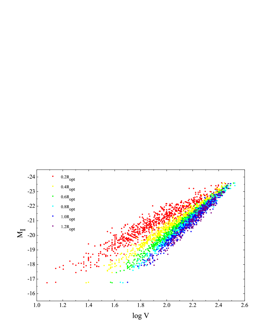
Figure 2: The Radial Tully-Fisher relations for the PS95 sample. Each one of the 6 relations is indicated with different color.

3 The Radial TF relationship

Given a sample of galaxies of magnitude $M_{band}$ and reliable rotational curves, the Radial Tully-Fisher (RTF further on) relation is defined, as the ensemble of the fitting relationships:

$$M_{band}=a_{n}\log V_{n}+b_{n}\,,$$ (9)

with $a_{n}$, $b_{n}$, the parameters of the fits and $R_{n}$ the radial coordinates at which the relationship is searched. The latter is defined for all object as a fixed multiple of the disk length-scale (or equivalently of $R_{opt}$). Parameters $a_{n}$, $b_{n}$ are estimated by the least squares method (without considering the velocity/magnitude uncertainties).

The existence of the Radial TF relation is clearly seen in Fig. 2 and Fig. 3, where all the TF-like relations for the PS95 sample are plotted together and identified with a different color. It is immediate to realize that they mark an ensemble of linear relations whose slopes and zero-points vary continuously with the reference radius $R_{n}$.

Independent Tully-Fisher like relationships exist in spirals at any ”normalized” radius $R_{n}$. We confirm this in a very detailed and quantitative way in the Figures 11, 12 and in the Tables 1, 2, 3, where very similar results are found for the other two samples. It is noticeable that the various investigations lead to the same consistent picture.

The slope $a_{n}$ increases monotonically with $R_{n}$; the scatter $s_{n}$ has a minimum at about two disk length-scales, $0.6R_{opt}$. In the $I$-band the values of the slopes are about 15$\%$ larger than those in the $r$-band. This difference, well known also for the standard TF, can be interpreted as due to the decrease, from the $r$ to the $I$ band, of the parameter $s$ (see Eq. 2), as effect of a different importance in the luminosity of the population of recently formed stars [Strauss & Willick 1995].

It is possible to compare the RTFs in different bands; in the case of absence of DM, true in the inner regions of spirals (except in the very luminous galaxies and LSB almost absent in our sample), for the reasonable values $s_{r}=0.1$ and $s_{I}=0$ the power law coefficient of the $L_{I}$ vs velocity relationship is larger by a factor $(0.5+s_{r})/(0.5+s_{I})$ than that of the $L_{r}$ vs velocity relationship, in details by a factor 1.2. This correction allows us to compare the $a_{n}$ slopes as a function of $R_{n}$ for our samples (see Figure 4). Remarkably, we find that the values of the slopes vary with $R_{n}$ according to a specific pattern: $b_{n}=-2.3-9.9(R_{n}/R_{opt})+3.9(R_{n}/R_{opt})^{2}$.

Figure 3: The Radial Tully-Fisher relation for the PS95 sample.

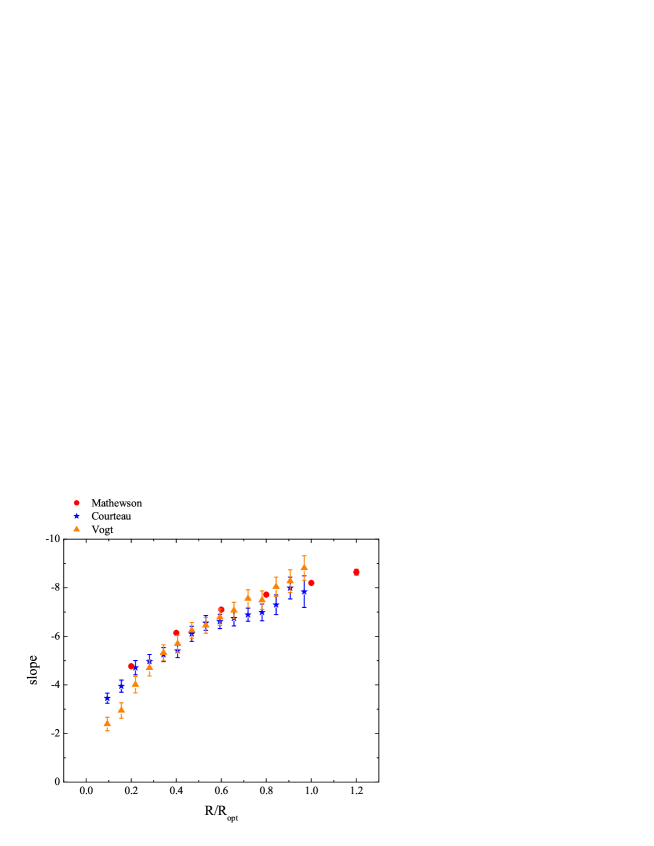
Figure 4: The slope of the Radial Tully-Fisher relation at different radii for the 3 samples. The slope for the standard TF is about to -7.5.

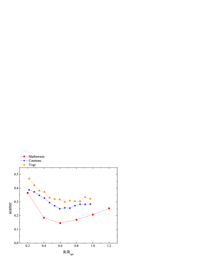
Figure 5: The scatter of the Radial Tully-Fisher relation at different radii for the 3 samples.

Figure 6: The $\%$ errors of the rotational velocity for different radii

It is worth to look at the scatter of the Radial TF relation (see Fig.5). We find that, near the galactic center the scatter is large $0.3-0.4$ dex, possibly due to a ”random” bulge component governing the local kinematics in this region being almost independent of the total galaxy magnitude. The scatter starts to decrease with $R_{n}$, to reach a minimum of $0.15-0.3$ dex at $R_{n}$ corresponding to two disk length scales, the radius where the contribution of the disk to the circular velocity $V(R)$ reaches the maximum. From $2R_{D}$ onward, the scatter increases outward reaching $0.3$ dex, at the farthest distances with available data, i.e. at 3-4 disk length-scales.

Figure 7: The standard TF relation for all 3 samples compered with the RTF relation at $R=0.6R_{opt}$.

Let us notice that these scatters are remarkably small. Most of the relations in the RTF family are statistically at least as significant as the standard TF relation, while the most correlated relationship, i.e. that at $2R_{D}$ shows a r.m.s of only 0.2 - 0.3 magnitudes (besides, significantly smaller than that of the standard TF (see Figure 6)). Since the r.m.s include also the effects of various observational errors, such small values could even indicate that the intrinsic scatter of the RTF relation at $\sim 2R_{D}$ is almost zero.

An important consequence of the smallness of the r.m.s of TF-like relationships is that we can claim that at any radius, the luminosity predicts the rotation velocity within the error of

$$\delta V_{n}/V_{n}=\ln(10)s_{n}/a_{n}\,.$$

This error (that includes also distance, inclination, and non circular motions errors) is remarkably small, mostly lying between 5%-10%, and not exceeding 20% even in the very inner bulge dominated regions (see figure for the PS95 sample). This result is an additional proof for the URC paradigm, even more impressive than the set of synthetic RC’s in PSS.

Incidentally, the existence of a radius ($R=0.6R_{opt}$) at which the TF-like relations show a minimum in the internal scatter is not related to the overall capability of the luminosity in predicting the rotation velocities. At very small $R\sim(0.1-0.2)R_{opt}$ the (random) presence of a bulge increases the scatter, in that, (as in ellipticals) the actual kinematical-photometric fundamental plane likely includes a third observational quantity (maybe the central surface density). At large $R$, the observed small increase of the scatter can be avoided by introducing small quadratic term in the eq (9).

The scatter of the RTF in the R band for the corresponding samples is somewhat larger than that in the I band for the PS95 sample. This can be easily explained by the following: i) the former samples include also a (small) fraction of Sa objects and their RCs are of higher spatial resolution (lower bin size) and therefore less efficient in smoothing the non-circular motion arisen by bars and spiral arms ii) the R band is more affected than the I Band by random recent episodes of star formation. A conservative estimate of these effects is $\sigma_{obs}\geq 0.2$, thus the intrinsic scatter of the RTF in the R band $(s_{n}^{2}-\sigma_{obs}^{2})^{0.5}$ results similar to that found in the I band.

4 Radial TF: implications

The marked systematic increase of the slopes of the RTF relationship, as their reference radius $R_{n}$ increases from the galaxy center to the stellar disk edge, bears very important consequences. First, it excludes, as viable mass models, those in which:

i) The gravitating mass follows the light distribution, due to a total absence of non baryonic dark matter or to DM being distributed similarly to the stellar matter. In both cases, in fact, we do not expect to find any variation of the slopes $a_{n}$ and very trivial variations of the zero points $b_{n}$ with the reference radius $R_{n}$, contrary to the evidence in Tables 1, 2, 3 and Fig. 4.

ii) The DM is present but with a luminosity independent fractional amount inside the optical radius. In this case, in fact, the value of the circular velocity at any reference radius $R_{n}$ will be a luminosity independent fraction of the value at any other reference radius (i.e. $\log V(R_{n})=k_{nm}+\log V(R_{m})$, $k_{nm}$ independent of luminosity). As a consequence the slopes $a_{n}$ in the RTF will be independent of $R_{n}$, while the zero-points $b_{n}$ will change in a characteristic way. It is clear that the evidence in Table 1, 2, 3 and Figure 4 contradicts this possibility.

The RTF contains crucial information on the mass distribution in spirals. In paper II we will fully recover and test it with theoretical scenarios. Here, instead, we will use a simple mass model (SMM), that includes a bulge, a disk and a halo mass component and it is tunable by means of 4 free parameters. By matching this model with the slopes of the RTF relation vs reference radii relationship (hereafter SRTF) we derive the gross features of the mass distribution in spirals. Let us point out, that this method has a clear advantage with respect to the mass modelling based on RCs. In this latter procedure, since the circular velocities have a quite limited variation with radius, physically different mass distributions may reproduce the observations equally well. Here instead, on one side, we will use an observational quantity, the slope of the RTF relation, that shows large variation with reference radius; on the other side, physically different mass distributions predict very different slope vs reference radius relationships.

First, without any loss of generality affecting our results, we assume the well known relationships among the crucial structural properties of spirals: i)

$$R_{D}=R_{1}l^{0.5}\,,$$

see PSS, with $l\equiv 10^{(M_{I}-M_{I}^{max})/2.5}$ and $M_{I}^{max}=-23.5$ the maximum magnitude of our sample, and ii)

$$M_{D}=M_{1}l^{1.3}\,,$$

(e.g. Shankar et al. 2006 and references therein). Notice that the constants $R_{1}$ and $M_{1}$ will play no role in the following. We will best fit the $a_{n}$ data, i.e. the SRTF relation shown in Fig (4) with the model function $a_{SMM}(x)$ derived from the SMM. In this way we will fix the free structural mass parameters.

We describe in detail the adopted SMM, the circular velocity is a sum of three contributions generated by the bulge component, taken as a point mass situated in the center, a Freeman disk, and a dark halo.

$$V^{2}_{SMM}(x)=GM_{D}/R_{D}[f_{d}(x)+{M_{b}\over M_{d}}{1\over(3.2x)}+{M_{halo}\over M_{D}}{1\over 3.2}f_{h}(x,\alpha)],$$

where $M_{halo}$ is the halo mass inside $R_{opt}$. It is useful to measure $V^{2}_{SMM}$ in units of $GM_{1}/R_{1}$, and to set it to be equal $1$.

The disk component from Eqs. (6) and (10), (11) takes the form:

$$V_{d}^{2}(x,l)=l^{0.8}f_{d}(x)\,,$$

with $V^{2}_{d}(1,1)=0.347$.

We set $M_{b}$ the bulge mass to be equal to a fraction $(c_{b}/(3.2\cdot 0.347)l^{0.5}$ of the disk mass, with $c_{b}$ a free parameter of the SMM and the exponent $0.5$ is suggested by the bulge-to disk vs total luminosity relation found for spirals. Then, we get

$$V_{b}^{2}(x)=c_{b}V_{d}^{2}(1,l)l^{0.5}x^{-1}\,.$$

The halo velocity contribution follows the profile of Eq. 7; at $R_{opt}$ it is set to be equal to $c_{h}/(3.2\cdot 0.347)l^{(k_{h}-0.5)}$ times the disk contribution $c_{b}$/$c_{h}$ and $k_{h}$, and $\alpha$ are the free parameters of the SMM.

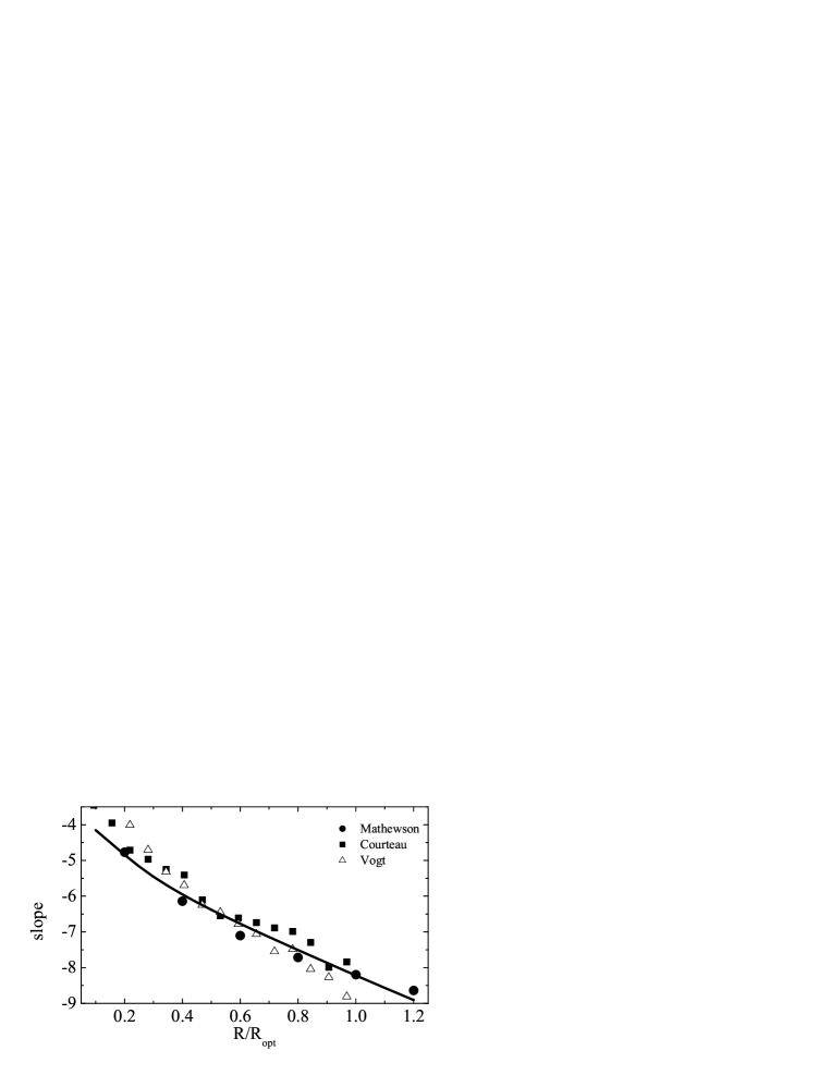
Figure 8: Slopes $a_{n}$ of the RTF for the 3 samples as a function of the reference radius in units of $R_{opt}$. The solid line is the best fit relation for Eq. 14

Then, we can write:

$$V_{SMM}^{2}(x,\alpha,l)=(c_{b}l^{1.3}/x+l^{0.8}f_{d}(x)+c_{h}l^{(k_{h}-0.5)}f_{h}(x,\alpha))\,,$$

where $f_{d}$ is given by Eq. (6), $f_{h}$ by Eq. (7). Notice that the simple form of $V_{SMM}$ allows us to get the predicted slope parameter $a_{SMM}(x)$.

The core radius $\alpha$ is a DM free parameter, however let us anticipate that, provided that this quantity lies between $0.5$ and $2$ (see Donato et al. 2004) it does not affect in a relevant way the SMM predictions. Instead the $a_{SMM}(x)$ relationship strongly depends on the values of $c_{h}$, $k_{h}$, $c_{b}$, and therefore they can be estimated with a good precision. We can reproduce the observational $a_{n}=a(R_{n})$ relationship, by means of the SMM (see Fig. 8) with the following best fit parameters values: i) $k_{h}=0.79\pm 0.04$, that means that less luminous galaxies have larger fraction of dark matter, ii) $c_{b}=0.13\pm 0.03$, and iii) $c_{h}=0.13\pm 0.06$ that indicates that at $(l,x)=(1,1)$ (i.e. inside $R_{opt}$), $20\%$ of the mass is in the bulge component, $20\%$ in the halo, while $60\%$ is in the stellar disk. The quoted uncertainties are the formal $\chi^{2}$ fitting uncertainties.

Figure 9: Baryonic mass fraction as a function of normalized radius for high and low luminosity objects.

Figure 10: Baryonic mass fraction at two different radii as a function of luminosity.

5 Discussion and conclusions

In spirals, at different galactocentric distances measured in units of disk length-scales $jR_{D}$ ($j=0.2,...,4$), there exists a family of independent Tully-Fisher-like relationships, $M_{band}=b_{j}+a_{j}\log V(R_{j})$, that we call the Radial Tully-Fisher relation, that contains crucial information on the mass distribution in these objects. In fact:

1) The RTF relationships show large systematic variations in their slopes $a_{j}$ (between $-4$ and $-8$) and a r.m.s. scatter generally smaller than that of the standard TF. This rules out the case in which the light follows the gravitating mass, and, in particular, all mass models that imply: a) an absence of dark matter, b) a single mass component c) the same dark-to-luminous-mass fraction within $jR_{D}$ in all galaxies.

2) The slopes $a_{j}$ decrease monotonically with $R_{j}$, implies the presence of a non luminous mass component whose dynamical importance, with respect to the stellar disk, increases with radius.

3) The existence of the RTF and the features of the slope vs $R_{j}$ can be well reproduced by means of a three components mass model that includes: a dark halo, with a core of radius $4R_{D}$ and mass $M_{halo}(R_{opt})\propto l^{0.7}$, a central bulge with $M_{bulge}\propto l^{1.8}$, an exponential thin disk of mass $M_{d}\propto l^{1.3}$ with, at $10^{11}L_{B,\odot}$, $60\%$ of the mass inside $R_{opt}$ in stellar form.

Let us also notice that we have produced a qualitatively new evidence for the presence of a luminosity dependent mass discrepancy in spirals, different from that obtained from the non Keplerian shapes of the RC’s. While, the latter originates from a failure: we do not observe the Keplerian fall-off of the circular velocities at the disk edge, and therefore we must postulate a new component, here, we provide a positive evidence for the existence of such dark component: we detect radial change of the slope and the scatter of existing relations between observables that positively indicates the presence of a more diffuse dark component.

The small scatter of the TF-like relationships in the inner regions of the spirals ($x=0.4-0.6$) has important implications for the DM halo core vs cusp controversy, more specifically on the claim that the observed rotation velocities $V(R)$ do not coincide with the circular velocities, i.e. with the equilibrium velocities associated with the central galaxy gravitational potential $\Phi$, $V_{circ}(R)=(-Rd\Phi/dR)^{1/2})$. It is claimed that, due non-circular/non-central motions, gas pressure gradients and other effects, $V(R)<V_{circ}$ by a substantial amount and models in which observed cored-solid body rotation curves $V(R)$ underly actual NFW-cusped circular velocities $V_{circ}(R)=V_{NFW}(R)\neq V(R)$ have been built (Hayashi 2006). Let us notice that this effect must be very large in that it must explain the large discrepancy between the observed rotation curves (taken as bona-fide circular velocities) and their NFW best fit mass models: the typical difference is

$$(V-V_{NFW})=(20-60)km/s$$

for galaxies with $V_{opt}=100-150$km/s (Gentile et al., Donato et al. and references therein). At $R_{n}=(0.4-0.6)R_{opt}$ we have $s_{n}\sim 0.3$, that certainly includes a component due to distance and inclinations errors. Even if we assume that its all due to the fact that $V\neq V_{circ}$ this would trigger a discrepancy of only $\sim 5-15$ km/s, far too small to account for the severe discrepancies of the NFW models.

Finally, let us stress that any model of formation of spiral galaxies must be able to produce (e.g. in the I band) a $M_{I}$ vs $\log V(2R_{D})$ relationship with a slope of $7\pm 0.1$ and an intrinsic scatter of $\leq 0.15$ magnitudes.

Acknowledgments

We thank S. Courteau and N. Vogt for kindly provided data. We also thank Gianfranco Gentile for helping us with preparation of this paper. We want to thank the anonymous referee for detailed comments that much improved the final version of this paper.

6 Appendix

In this appendix we present tables and figures related to our result and the galaxies of Samples 2 and 3.

Table 1: Parameters of the Radial Tully-Fisher relation at different radii for the Mathewson sample

$R/R_{opt}$	zero point	error	slope	error	SD	N
0.2	-11.78	0.103	-4.77	0.054	0.366	739
0.4	-8.241	0.068	-6.141	0,033	0.185	786
0.6	-5.787	0.063	-7.102	0.029	0.146	794
0.8	-4.22	0.09	-7.718	0.042	0.17	657
1.0	-3.034	0.146	-8.197	0.067	0.208	447
1.2	-1.979	0.261	-8.639	0.118	0.253	226

column 1 - the isophotal radius,
column 2 - intercept value $b_{n}$,
column 3 - the standard error of $b_{n}$,
column 4 - the slope $a_{n}$,
column 5 - the standard error of $a_{n}$,
column 6 - the scatter,
columns 7 - the number of observational points

Table 2: Parameters of the Radial TF relation at different radii for the Courteau sample

$R/R_{opt}$	zero point	error	slope	error	SD	N
0.03	-18.217	0.287	-1.8	0.189	0.516	75
0.09	-15.615	0.39	-2.878	0.209	0.381	74
0.16	-14.355	0.495	-3.336	0.249	0.388	75
0.22	-13.379	0.55	-3.707	0.27	0.397	76
0.28	-12.155	0.741	-4.194	0.355	0.465	79
0.34	-11.7	0.613	-4.374	0.291	0.361	74
0.41	-11.11	0.617	-4.586	0.289	0.338	72
0.47	-9.962	0.674	-5.086	0.31	0.295	68
0.53	-9.114	0.699	-5.445	0.321	0.296	71
0.59	-8.919	0.733	-5.519	0.334	0.293	68
0.66	-8.623	0.752	-5.61	0.341	0.279	65
0.72	-8.351	0.625	-5.737	0.284	0.255	63
0.78	-8.172	0.763	-5.799	0.345	0.274	61
0.84	-7.329	1.0	-6.152	0.456	0.32	53
0.91	-6.372	1.0	-6.58	0.449	0.286	44
0.97	-7.573	1.54	-6.042	0.688	0.31	37
1.03	-7.728	1.993	-5.984	0.888	0.311	25
1.09	-9.265	2.254	-5.307	1.0	0.212	14
1.16	-6.853	1.767	-6.35	0.789	0.281	15

Table 3: Parameters of the Radial Tully-Fisher relation at different radii for the Vogt sample

$R/R_{opt}$	zero point	error	slope	error	SD	N
0.09	-19.351	0.526	-1.992	0.278	0.55	78
0.16	-18.118	0.64	-2.456	0.316	0.528	78
0.22	-16.142	0.714	-3.309	0.339	0.472	76
0.28	-14.787	0.728	-3.869	0.338	0.43	77
0.34	-13.583	0.73	-4.365	0.334	0.394	77
0.41	-12.646	0.78	-4.747	0.354	0.386	77
0.47	-11.746	0.784	-5.112	0.353	0.365	77
0.53	-11.342	0.805	-5.264	0.361	0.361	75
0.59	-10.698	0.778	-5.51	0.347	0.327	72
0.66	-9.804	0.77	-5.885	0.341	0.309	71
0.72	-9.244	0.83	-6.125	0.368	0.318	70
0.78	-9.227	0.936	-6.104	0.414	0.341	68
0.84	-7.873	0.906	-6.7	0.4	0.304	60
0.91	-7.435	1.057	-6.893	0.466	0.334	58
0.97	-6.377	1.153	-7.343	0.505	0.323	50
1.03	-8.398	1.414	-6.435	0.62	0.345	41
1.09	-7.953	1.377	-6.628	0.599	0.301	35
1.16	-8.683	1.38	-6.947	0.622	0.228	24
1.22	-9.616	1.444	-6.842	0.714	0.275	23
1.28	-7.394	2.467	-6.834	1.072	0.347	16

Table 4: Parameters of the standard Tully-Fisher relation for 3 samples.

Data	zero point	error	slope	error	SD	N
Mathewson	-4.455	0.15	-7.57	0.069	0.327	841
Courteau	-8.398	1.26	-5.526	0.556	0.495	81
Vogt et al.	-8.277	0.997	-6.423	0.433	0.389	79

Figure 11: The Radial Tully-Fisher relation for the Courteau sample.

Figure 12: The Radial Tully-Fisher relation for the Vogt sample.

Names of galaxies from the Courteau sample: UGC 10096, UGC 10196, UGC 10210, UGC 10224, UGC 1053, UGC 10545, UGC 10560, UGC 10655, UGC 10706, UGC 10721, UGC 10815, UGC 11085, UGC 11373, UGC 1152, UGC 11810, UGC 12122, UGC 12172, UGC 12200, UGC 12294, UGC 12296, UGC 12304, UGC 12325, UGC 12354, UGC 12598, UGC 12666, UGC 1426, UGC 1437, UGC 1531, UGC 1536, UGC 1706, UGC 1812, UGC 195, UGC 2185, UGC 2223, UGC 2405, UGC 2628, UGC 3049, UGC 3103, UGC 3248, UGC 3269, UGC 3270, UGC 3291, UGC 3410, UGC 346, UGC 3652, UGC 3741, UGC 3834, UGC 3944, UGC 4232, UGC 4299, UGC 4326, UGC 4419, UGC 4580, UGC 4779, UGC 4996, UGC 5102, UGC 540, UGC 562, UGC 565, UGC 5995, UGC 6544, UGC 6692, UGC 673, UGC 7082, UGC 732, UGC 7549, UGC 7749, UGC 7810, UGC 7823, UGC 783, UGC 784, UGC 8054, UGC 8118, UGC 8707, UGC 8749, UGC 8809, UGC 890, UGC 9019, UGC 9366, UGC 9479, UGC 9598, UGC 9745, UGC 9753, UGC 9866, UGC 9973

Names of galaxies from the Vogt sample: UGC 927, UGC 944, UGC 1033, UGC 1094, UGC 1437, UGC 1456,UGC 1459, UGC 2405, UGC 2414, UGC 2426, UGC 2518, UGC 2618, UGC 2640, UGC 2655, UGC 2659, UGC 2700, UGC 3236, UGC 3270, UGC 3279, UGC 3289, UGC 3291, UGC 3783, UGC 4275, UGC 4287, UGC 4324, UGC 4607, UGC 4655, UGC 4895, UGC 4941, UGC 5166, UGC 5656, UGC 6246, UGC 6437, UGC 6551, UGC 6556, UGC 6559, UGC 6718, UGC 6911, UGC 7845, UGC 8004, UGC 8013, UGC 8017, UGC 8108, UGC 8118, UGC 8140, UGC 8220, UGC 8244, UGC 8460, UGC 8705, UGC 10190, UGC 10195, UGC 10459, UGC 10469, UGC 10485, UGC 10550, UGC 10981, UGC 11455, UGC 11579, UGC 12678, UGC 12755, UGC 12792, UGC 150059, UGC 180598, UGC 210529, UGC 210559, UGC 210629, UGC 210634, UGC 210643, UGC 210789, UGC 211029, UGC 220864, UGC 221174, UGC 221206, UGC 251400, UGC 260640, UGC 260659, UGC 330781, UGC 330923, UGC 330925, UGC 330996, UGC 331021

References

- [Aaronson et al. 1982] Aaronson, M., et al.,1982, ApJS, 50, 241
- [Courteau 1996] Courteau, S., 1996, ApJS, 103, 363
- [Courteau 1997] Courteau, S., 1997, AJ, 114, 2402
- [Donato 2004] Donato, F., Gentile, G., Salucci, P., 2004, MNRAS, 353L, 17
- [Federspiel et al. 1994] Federspiel, M., Sandage, A., Tammann, G. A., 1994, ApJ, 430, 29
- [Freeman 1970] Freeman, K.C., 1970, ApJ, 160, 811
- [Gentile 2004] Gentile G., Salucci P., Klein U., Vergani D., Kalberla P., 2004, MNRAS, 351, 903
- [Hayashi et al. 2006] Hayashi E., Navarro J.F., Springel V., astro-ph/0612327
- [Mathewson et al. 1992] Mathewson, D. S., Ford, V. L., Buchhorn, M., 1992, ApJS, 81, 413
- [Mathewson et al. 1992] Mathewson, D. S., Ford, V. L., Buchhorn, M., 1992, ApJ, 389L, 5
- [Mathewson et al. 1996] Mathewson, D. S., Ford, V. L., 1996, ApJS, 107, 97
- [Persic & Salucci 1988] Persic M., Salucci P., 1988, MNRAS, 234, 131
- [Persic & Salucci 1995] Persic, M., Salucci, P., 1995, ApJS, 99, 501, PS95
- [Persic & Salucci 1996] Persic, M., Salucci, P., Stel, F., 1996, MNRAS, 281, 1, 27-47, PSS
- [Pierce & Tully 1988] Pierce, M., Tully, R. B., 1988, ApJ, 330, 579
- [Pierce & Tully 1992] Pierce, M., Tully, R. B., 1992, Apj 387,47
- [Rhee 1996] Rhee, M., H., 1996, Phd Thesis, Groningen
- [Salucci et al. 2003] Salucci P., Walter F., Borriello A., 2003, A&A, 409, 53
- [Salucci & Gentile 2005] Salucci, P., Gentile, G., astro-ph/0510716, in press in Phys.Rew.Lett.D 2006
- [Salucci et al. 1993] Salucci, P., Frenk, C. S., Persic, M., 1993, MNRAS, 262, 392
- [Shankar et al. 2006] Shankar, F., Lapi, A., Salucci, P., De Zotti, G., Danese, L., astro-ph/0601577
- [Strauss & Willick 1995] Strauss, M. A., Willick, J. A., 1995, Physics Reports, 261, 271
- [Tully & Fisher 1977] Tully, R. B., Fisher, J. R., 1977, A&A, 54, 661
- [Vogt et al. 2004] Vogt, N. P., Haynes, M. P., Herter, T., Giovanelli, R., 2004, AJ, 127, 3273
- [Vogt et al. 2004] Vogt, N. P., Haynes, M. P., Herter, T., Giovanelli, R., 2004, AJ, 127, 3325