Hot Jupiter Variability in Eclipse Depth

Abstract

Physical conditions in the atmospheres of tidally locked, slowly rotating hot Jupiters correspond to dynamical circulation regimes with Rhines scales and Rossby deformation radii comparable to the planetary radii. Consequently, the large spatial scales of moving atmospheric structures could generate significant photospheric variability. Here, we estimate the level of thermal infrared variability expected in successive secondary eclipse depths, according to hot Jupiter turbulent “shallow-layer” models. The variability, at the few percent level or more in models with strong enough winds, is within the reach of Spitzer measurements. Eclipse depth variability is thus a valuable tool to constrain the circulation regime and global wind speeds in hot Jupiter atmospheres.

1 Introduction

The regime of circulation in hot Jupiter atmospheres may be unlike any of the familiar cases in the Solar System. Hot Jupiters are gaseous giant planets found in close, circular orbits around their parent stars, with periods on the order of a few days (e.g., Butler et al., 2006). General arguments suggest that these planets should be tidally locked (Guillot et al., 1996; Rasio et al., 1996; Lubow et al., 1997; Ogilvie & Lin, 2004): their permanent day-sides are then continuously subject to intense stellar irradiation, while night-sides are only subject to modest internal energy fluxes. Given such an uneven energetic forcing, atmospheric winds would tend to redistribute heat around the planet. The nature and efficiency of this redistribution process is important in determining a variety of hot Jupiter observational properties (e.g., Seager et al., 2005; Burrows et al., 2005; Fortney et al., 2005; Barman et al., 2005; Iro et al., 2005; Burrows et al., 2006; Fortney et al., 2006).

Two groups have attempted to address the global atmospheric circulation problem in hot Jupiter atmospheres, using different approaches (Showman & Guillot, 2002; Cho et al., 2003; Menou et al., 2003; Cooper & Showman, 2005). On dynamical grounds, it was argued in Menou et al. (2003, see also Showman & Guillot 2002), and explicitly shown via turbulent shallow-layer simulations in Cho et al. (2003, 2006), that tidally locked hot Jupiters occupy a regime of circulation that is qualitatively different from that of Solar System giant planets. The few bands and prominent circumpolar vortices emerging in these simulations can be understood in terms of the large Rhines scale and Rossby deformation radius in these atmospheres (e.g., Cho & Polvani, 1996a, b). Menou et al. (2003) suggested that the large resulting spatial scales of moving circulation structures could lead to detectable hot Jupiter variability.

Soon, interesting observational constraints will be placed on these circulation regime arguments. Three hot Jupiters have been detected through infrared secondary eclipses with the Spitzer Space Telescope: HD189733b (Deming et al., 2006), HD209458b (Deming et al., 2005), and TrES-1 (Charbonneau et al., 2005). The planetary day-side flux is deduced from the eclipse depth measured when the planet is hidden behind its star. Repeated eclipse measurements could thus reveal detectable levels of variability of the planetary day-side flux in these three systems. In this Letter, we quantify the level of thermal infrared variability expected in secondary eclipse depths, according to the shallow-layer models of Cho et al. (2003, 2006).

2 Shallow-Layer Circulation Models

As explained in detail in Cho et al. (2003, 2006), turbulent equivalent-barotropic models published to date greatly emphasize dynamical aspects of hot Jupiter atmospheric circulation. We adopt the same notation and adiabatic models as in Cho et al. (2006): the global wind strength, $\bar{U}$, and the net amplitude of radiative forcing, $\eta$, are parameterized, not predicted. However, given these two (and other relevant global planetary) parameters, the turbulent atmospheric circulation is consistently found to develop a broad equatorial wind and two large circumpolar vortices revolving around the poles in several planetary days (= orbits). The dynamically modified layer thickness in these models is a proxy for the planet’s photospheric temperature field. We refer the reader to Cho et al. (2006) for details on the models, as well as a vast exploration of their parameter space.

Our limited goal here is to show that the thermal variability expected in at least some of these models is sufficiently large to be detectable via repeated Spitzer secondary eclipse measurements. Consequently, we focus on a limited set of four models, with global wind speed values from $\bar{U}=100$ to $800$ m s^-1 and a moderate amplitude of radiative forcing, $\eta=0.05$ (allowing the weak thermal contrast of features in slow wind models to remain apparent).

The models are explicitly calculated for HD209458b parameters, at moderate T63 ($192\times 96$ grid) resolution, over a hundred planetary days or more. Resolution tests (up to T170) show that T63 is sufficient to capture atmospheric temperature features well enough for our present purpose. Daily outputs from the simulations are used to generate model temperature maps of the day-side thermal emission in our variability study (see below). Table 1 summarizes the range of photospheric temperatures derived from these four models, for the two brightest planets in our study.

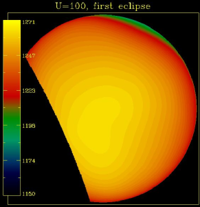
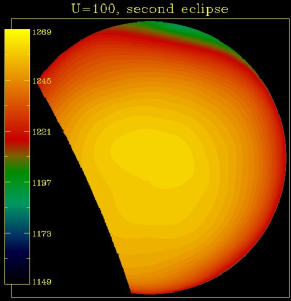
Figure 1: Partially eclipsed temperature maps (in K) in a HD209458b model with a $100$ m s^-1  global wind speed, for two successive eclipses. Little thermal infrared variability is expected.

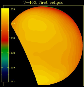
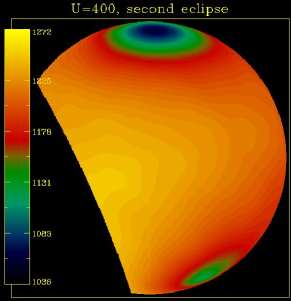
Figure 2: Same as Fig. 1 in a model with a $400$ m s^-1 global wind speed. Significant thermal infrared variability is expected in this case.

Figures 1 and 2 show snapshots of orthographically projected, day-side temperature maps in HD209458b models with $\bar{U}=100$ and $400$ m s^-1, respectively, for two successive eclipses (i.e. after one HD209458b day). These projections illustrate how thermal variability in total eclipse depth is expected, from one eclipse to the next, if large, high contrast temperature features, associated with moving circulation structures, are present (in particular, the cyclonic circumpolar vortices most obviously visible in Fig. 2). Each temperature map in Figs. 1 and 2 is shown partially eclipsed, for the specific geometry of the HD209458 system. According to these circulation models, cold polar vortices have relatively small (apparent) areas, so that the magnitude of their contribution to a variable eclipsed day-side flux is unclear without a detailed calculation.

3 Thermal Variability in Eclipse Depth

Our method to calculate eclipse depths in models like the ones shown in Figs. 1 and 2 follows very closely that used in Rauscher et al. (2007) to study partial eclipse diagnostics. Planet-daily outputs from the circulation simulations provide the temperature fields used to model successive eclipses. Accounting for system specific inclination and geometry, these temperature fields are orthographically projected onto a 2D disk discretized with ($100$, $200$) resolution elements in ($r$,$\theta$). To calculate spectra, we assume that the vertical temperature profile follows radiative equilibrium according to the cloudless models of Seager et al. (2005), under the assumption that the local flow temperature from the circulation model equals the effective temperature in the radiative model. We then integrate the spectral emission contributed by each apparent surface element on the planetary disk, in the global range of effective temperatures from $700$ to $2000$ K. Monochromatic fluxes at Earth are then integrated over Spitzer spectral bands (for IRAC, IRS, and MIPS) to predict the corresponding successive eclipse depths. In the future, it will be important to improve upon this simple treatment by fully incorporating radiative transfer in circulation models.

As in Rauscher et al. (2007), we also perform an idealized, bolometric blackbody analysis, to avoid relying exclusively on model specific features of the cloudless spectral emission models used. In these simpler blackbody models, the bolometric flux contributed by each planetary disk surface element is scaled as the fourth power of the local photospheric temperature.

Figure 3a shows relative variations in successive eclipse depths predicted by the four HD209458b circulation models, assuming simple bolometric blackbody emission. Variations are semi-periodic, as expected from the quasi-periodic motion of the circumpolar vortices around the planet. As the magnitude of the global wind speed, $\bar{U}$, is increased from $100$ to $800$ m s^-1, leading to higher contrast motion-induced temperature structures, the amplitude of thermal infrared variability also increases, from a few % to $\sim 60$-$70$%. Figure 3b shows eclipse depth variations for the HD209458b model with $\bar{U}=400$ m s^-1 as before, but this time using the detailed spectral emission models to calculate contributions in various Spitzer bands. While the overall variability scale is similar, it is clear that, by using Spitzer bands, one preferentially filters emission from a selective range of temperatures on the planetary disk, which contribute to varying levels of variability. The effect is substantial and we find that variability is the strongest in shortest wavelength Spitzer bands, where thermal contrast from the cold circumpolar vortices is the highest.

We calculated explicit circulation models only for HD209458b but we can use the general dynamical similarity of hot Jupiter atmospheres (Menou et al., 2003) to rescale simply our results for HD189733b and TrES-1. Assuming identical dynamics but allowing for different average atmospheric temperatures, we linearly rescale our model temperature maps proportionally to the zero albedo, fully redistributed equilibrium temperature, $T_{p}$, of the other two planets (as in Rauscher et al., 2007). We find that the eclipse depth variability properties for HD189733b and TrES-1 do not deviate from those of HD209458b by more than $\sim 10$%. Increasing planetary albedos also has little effects on the variability properties, as long as albedos remain $\ll 1$. Finally, as a matter of generality, we have checked that arbitrarily varying any system’s orbital inclination in the range 80-90^o  has little effect on its variability properties.

4 Detecting Eclipse Depth Variability

We now address the feasibility of detecting variability in eclipse depth, at the level predicted by the above models, with Spitzer. Let us define $\sigma_{ed}$ as the fractional error on the eclipse depth, that is the ratio of the full (1-$\sigma$) error on the eclipsed flux to the eclipsed flux itself. Values of $\sigma_{ed}$ for the existing secondary eclipse measurements (taken from Charbonneau et al., 2005; Deming et al., 2005, 2006) are listed in bold in Table 2. These numbers already suggest that eclipse depth variability at the level of $5$-$20$% could be detected in these systems.

Our variability models indicate, however, that specific Spitzer bands may be much more useful than others for eclipse depth variability detections. We perform simple estimates of $\sigma_{ed}$ errors for any combination of Spitzer instrument and hot Jupiter system as follows. We use the same set of system parameters as in Table 1 of Rauscher et al. (2007). Assuming that errors on the non-eclipsed flux are comparatively very small, we write $\sigma_{ed}=\sigma_{1}/\sqrt{N}$, where $\sigma_{1}$ is the noise per data point in units of the eclipsed flux and $N$ is the number of single data points collected during a full eclipse period. $N$ is the ratio of the secondary eclipse duration to the instrumental cadence (taken from existing measurements). The eclipse duration time is calculated as $t_{\rm ec}={2}\sqrt{(R_{*}+R_{p})^{2}-a^{2}\sin^{2}(90^{\mathrm{o}}-i)}/v$, where $v=2\pi a/P$ is the planet’s orbital velocity, $P$ its orbital period, $a$ its orbital semi-major axis, $i$ is the orbital inclination, and $R_{*}$ and $R_{p}$ are the stellar and planetary radii, respectively (see Table 1 of Rauscher et al., 2007). We obtain values of $t_{\rm ec}=1.76$, $3.23$ and $2.55$ hrs for HD189733b, HD209458b and TrES-1, respectively.

Finally, we extrapolate instrument-specific $\sigma_{ed}$ errors known for one system to the other two systems of interest by assuming blackbody emission for both the star and the planet. This results in the following instrument-specific scaling between systems A and B:

$$\frac{\sigma_{ed}^{B}}{\sigma_{ed}^{A}} = \sqrt{\frac{t_{ec}^{A}}{t_{ec}^{B}}}\sqrt{\frac{F_{*}^{B}}{F_{*}^{A}}}\left(\frac{F_{p}^{A}}{F_{p}^{B}}\right)$$

$$= \sqrt{\frac{t_{ec}^{A}}{t_{ec}^{B}}}\left(\frac{d_{B}}{d_{A}}\right)\left(\frac{R_{p}^{A}}{R_{p}^{B}}\right)^{2}\left(\frac{R_{*}^{B}}{R_{*}^{A}}\right)\left(\frac{B_{\lambda}(T_{p}^{A})}{B_{\lambda}(T_{p}^{B})}\right)\sqrt{\frac{B_{\lambda}(T_{*}^{B})}{B_{\lambda}(T_{*}^{A})}},$$

where $d$ is the distance to the system and $B_{\lambda}$ is the Planck function evaluated at the central wavelength of the instrumental band under consideration. $T_{*}$ is the stellar effective temperature and $T_{p}=T_{*}\sqrt{R_{*}/2a}$ is the fully redistributed planetary equilibrium temperature calculated in the small albedo limit, exactly as in Rauscher et al. (2007). The resulting extrapolated values of $\sigma_{ed}$ for the three systems of interest are listed in Table 2.

Repeated eclipse depth measurements with IRAC for HD189733b and HD209458b appear to be the most likely to succeed in detecting atmospheric variability, at the few percent level or more. Such variability measurements would be difficult for TrES-1. Figure 3 shows that any pair of successive eclipses will generally not display the full range of variability amplitude: more than two eclipse measurements are needed to sample variability properties adequately. This requirement can be quantified by calculating distributions of fractional variations in eclipse depth over series of 2, 3, 4 or more successive eclipse measurements. Comparing these distributions of eclipse depth variations to the (1-$\sigma_{ed}$) errors listed in Table 2, we find that detecting the eclipse depth variability predicted by the $\bar{U}=$400 or 800 m s^-1 models at the 2-3 $\sigma$ level requires 3-4 IRAC eclipses (at 4.5 or, slightly better, at 8µm). A generally larger number of eclipses is needed to detect the variability predicted by models with smaller global wind speeds. Eclipse depth variations at the level predicted by the $\bar{U}=$100 m s^-1 model would be systematically masked by eclipse depth measurement uncertainties, according to our estimates. Finally, we note that a sufficiently large number of successive eclipse measurements could reveal the quasi-periodicity apparent in Fig. 3.

5 Discussion and Conclusion

We have illustrated, using simple turbulent shallow-layer circulation models, how eclipse depth variability can be used to constrain the circulation regime and global wind speeds in hot Jupiter atmospheres.

Clearly, our circulation models and variability predictions are highly idealized. We have focused on simple thermal diagnostics in models describing an atmosphere as a single horizontal layer of turbulent fluid. Issues related to detailed radiative transfer (e.g., variation of photospheric height with wavelength; Iro et al., 2005; Seager et al., 2005; Harrington et al., 2006), the presence of high-altitude haze or the possible existence of clouds could all seriously affect our conclusions. Even strictly within the framework of our shallow-layer models, we know that the parameterized amplitude of net radiative forcing, $\eta$, can affect the thermal contrast, and therefore the detectability, of moving atmospheric structures (see Cho et al., 2006, for details). We have recalculated all our circulation and variability models with increased values of $\eta=0.1$ and $0.2$. We find that the variability amplitude is reduced by up to a factor of two from the case with $\eta=0.05$ shown in Fig. 3. Values of $\eta>0.2$ would further reduce the variability amplitude. In the future, multi-wavelength phase curve data (e.g., Harrington et al., 2006) may provide useful observational diagnostics on the relevant value of $\eta$ for a given planet.

Despite these shortcomings, our results are promising in showing that eclipse depth variability is a new and potentially powerful tool to diagnose circulation and wind speeds in hot Jupiter atmospheres. In the future, as more refined atmospheric models are developed and more data becomes available, this tool should become increasingly useful in characterizing hot Jupiter atmospheres.

We thank an anonymous referee for comments that helped improve the manuscript. This work was supported by NASA contract NNG06GF55G, NASA Astrobiology Institute contract NNA04CC09A and a Spitzer Theory grant. q

Table 1: Cho et al. (2006) models under consideration

		Min-Max Temperature (K)
	$\bar{U}$ (m s-1)	HD209458b	HD189733b
Model 1	100	1147-1275	956-1062
Model 2	200	1112-1287	926-1072
Model 3	400	1006-1308	838-1088
Model 4	800	669-1372	557-1141

Table 2: Measured (in bold) and estimated values of $\sigma_{ed}$.

Instrument, wavelength	HD 189733b	HD 209458b	TrES-1
IRAC, 4.5 µm	0.018	0.039	0.20
IRAC, 8 µm	0.014	0.026	0.16
IRS, 16 µm	0.055	0.11	0.62
MIPS, 24 µm	0.086	0.18	0.96

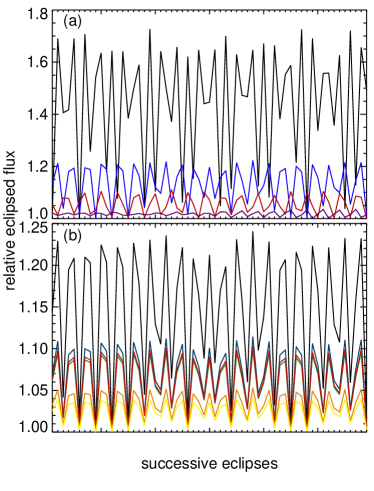
Figure 3: Relative flux variations at full eclipse according to HD209458b circulation models. Discrete points are connected for clarity and fluxes are normalized to the minimum value in each case. (a) Variations for simple bolometric blackbody emission, in models with $\bar{U}$=100 (purple line), 200 (red), 400 (blue), and 800 m s^-1 (black). (b) Variations according to detailed spectral emission models, in various Spitzer bands, for the $\bar{U}$=400 m s^-1 model of HD209458b. From top to bottom, the curves correspond to 3.6µm (black), 4.5µm (blue), 8µm (red), 6µm (green), 16µm (orange), and 24µm (yellow).

References

- Barman et al. (2005) Barman, T. S., Hauschildt, P. H., & Allard, F. 2005, ApJ, 632, 1132
- Burrows et al. (2005) Burrows, A., Hubeny, I., & Sudarsky, D. 2005, ApJ, 625, L135
- Burrows et al. (2006) Burrows, A., Sudarsky, D., & Hubeny, I. 2006, ApJ, 650, 1140
- Butler et al. (2006) Butler, R. P. et al. 2006, ApJ, 646, 505
- Charbonneau et al. (2005) Charbonneau, D., et al. 2005, ApJ, 626, 523
- Cho et al. (2003) Cho, J. Y.-K., Menou, K., Hansen, B. M. S., & Seager, S. 2003, ApJ, 587, L117
- Cho et al. (2006) Cho, J. Y.-K., Menou, K., Hansen, B., & Seager, S. 2006, ApJ submitted, astro-ph/0607338
- Cho & Polvani (1996a) Cho, J. Y.-K. & Polvani, L. M. 1996a, Phys. Fluids, 8, 1531
- Cho & Polvani (1996b) Cho, J. Y.-K. & Polvani, L. M. 1996b, Science, 273, 335
- Cooper & Showman (2005) Cooper, C. S., & Showman, A. P. 2005, ApJ, 629, L45
- Deming et al. (2006) Deming, D., Harrington, J., Seager, S., & Richardson, L. J. 2006, ApJ, 644, 560
- Deming et al. (2005) Deming, D., Seager, S., Richardson, L. J., & Harrington, J. 2005, Nature, 434, 740
- Guillot et al. (1996) Guillot, T., Burrows, A., Hubbard, W. B., Lunine, J. I., & Saumon, D. 1996, ApJ, 459, L35
- Harrington et al. (2006) Harrington, J. et al. 2006, Science, 314, 623
- Fortney et al. (2005) Fortney, J. J., Marley, M. S., Lodders, K., Saumon, D., & Freedman, R. 2005, ApJ, 627, L69
- Fortney et al. (2006) Fortney, J. J., Cooper, C. S., Showman, A. P., Marley, M. S.& Freedman, R. 2006, ApJin press, astro-ph/0608235
- Iro et al. (2005) Iro, N., Bezard, B. & Guillot, T 2005, A&A, 436, 719
- Lubow et al. (1997) Lubow, S. H., Tout, C. A., & Livio, M. 1997, ApJ, 484, 866
- Menou et al. (2003) Menou, K. Cho, J. Y.-K., Seager, S. & Hansen, B. M. S. 2003, ApJ, 587, L113
- Ogilvie & Lin (2004) Ogilvie, G. I., & Lin, D. N. C. 2004, ApJ, 610, 477
- Rasio et al. (1996) Rasio, F. A., Tout, C. A., Lubow, S. H., & Livio, M. 1996, ApJ, 470, 1187
- Rauscher et al. (2007) Rauscher, E., Menou, K., Seager, S., Deming, D., Cho, J. Y.-K., & Hansen, B. M. S. 2007, ApJ submitted
- Seager et al. (2005) Seager, S., Richardson, L. J., Hansen, B. M. S., Menou, K., Cho, J. Y.-K., & Deming, D. 2005, ApJ, 632, 1122
- Showman & Guillot (2002) Showman, A. P. & Guillot, T. 2002, A&A, 385, 166