Toward Eclipse Mapping of Hot Jupiters

Abstract

Recent Spitzer infrared measurements of hot Jupiter eclipses suggest that eclipse mapping techniques could be used to spatially resolve the day-side photospheric emission of these planets using partial occultations. As a first step in this direction, we simulate ingress/egress lightcurves for three bright eclipsing hot Jupiters and evaluate the degree to which parameterized photospheric emission models can be distinguished from each other with repeated, noisy eclipse measurements. We find that the photometric accuracy of Spitzer is insufficient to use this tool effectively. On the other hand, the level of photospheric details that could be probed with a few JWST eclipse measurements could greatly inform hot Jupiter atmospheric modeling efforts. A JWST program focused on non-parametric eclipse map inversions for hot Jupiters should be actively considered.

1 Introduction

Eclipses can be used as powerful tools to spatially resolve the photospheric emission properties of astronomical objects. During ingress and egress, the partial occultation effectively maps the photospheric emission region of the object being eclipsed. With arbitrarily high photon statistics, the (spatial) resolving power attainable with such an astronomical telescope is unrivaled. In the past, eclipse mapping methods have thus been used with great success to measure limb darkening laws on stellar companions (e.g. Warner et al., 1971), to map the surface appearance of Pluto (see review by Stern, 1992), or to confirm the Keplerian nature of accretion disks in Cataclysmic Variables, on the basis of their radial emission profiles (e.g. Rutten, 1996). Given the recent Spitzer measurements of infrared eclipses for three hot Jupiters (Deming et al., 2005, 2006; Charbonneau et al., 2005), it is natural to explore the potential for eclipse mapping of hot Jupiters (Williams et al., 2006).

The regime of atmospheric circulation present on hot Jupiters may be unlike any of the familiar cases encountered in the Solar System. Hot Jupiters are massive, gaseous giant planets found in close, circular orbits around their parent stars, with orbital periods on the order of a few days (e.g. Butler et al., 2006). General arguments suggest that these planets are tidally locked (Rasio et al., 1996; Lubow et al., 1997; Ogilvie & Lin, 2004), so that their permanent day-sides are continuously subjected to intense stellar irradiation, while their night-sides may be heated only by a much more modest internal energy flux. In the presence of such an uneven energetic forcing, leading to significant (horizontal) temperature gradients, atmospheric winds will attempt to redistribute the heat more evenly around the planet. The efficiency of this horizontal heat redistribution is an important open question for hot Jupiters as it largely determines their observational properties. Several attempts have been made to address this general circulation problem for hot Jupiter atmospheres, using different approaches (Showman & Guillot, 2002; Cho et al., 2003; Menou et al., 2003; Cooper & Showman, 2005, see also Burkert et al. 2005), and interesting constraints are now being placed on these models through the recent infrared measurements.

Three hot Jupiters have been directly detected in infrared with the Spitzer Space Telescope: HD189733b (Deming et al., 2006), HD209458b (Deming et al., 2005), and TrES-1 (Charbonneau et al., 2005). The planetary day-side flux is deduced from the secondary eclipse depth, when the planet is hidden behind its star. Based on such flux measurements at different wavelengths, several groups have computed spectral emission models for various prescribed levels of heat redistribution and concluded that at least some amount of heat redistribution must be present (Seager et al., 2005; Burrows et al., 2005; Fortney et al., 2005; Barman et al., 2005; Burrows et al., 2006; Fortney et al., 2006). These secondary eclipse constraints remain weak at the moment but they could rapidly improve in quality in the future. In addition, a first hot Jupiter infrared orbital phase curve for the non-eclipsing planet Ups And b has been reported very recently (Harrington et al., 2006). The large inferred amplitude of the phase curve, measuring the day- to night-side temperature difference, suggests a rather weak role for heat redistribution in this case. More work is likely needed to interpret the phase curve reliably, and in particular to address the complications that may arise from the existence of different regimes of heat redistribution at different heights in the atmosphere (e.g. Seager et al., 2005; Iro et al., 2005; Cooper & Showman, 2005).

This recent progress in direct infrared detections of hot Jupiters leads us to consider the possibility that eclipse mapping techniques could also be used in these systems (see also Williams et al., 2006). Contrary to existing measurements, which only constrain disk-integrated quantities, eclipse mapping of a hot Jupiter can provide a “spatially resolved map” of its day-side photospheric disk, with “pixel” shapes and sizes determined by eclipse geometry and photometric accuracy. In principle, one can measure the emission of any individual “pixel” directly from the shape of the ingress and egress lightcurves, without making any significant assumption on the nature of the photospheric emission itself. Such “non-parametric” inversion techniques can be used in the eclipse mapping context (e.g. Horne, 1985; Spruit, 1994; Rutten, 1996, 1998; Bobinger, 2000; Baptista, 2001), but in this first study we focus on a much simpler parametric method to evaluate the accuracy with which details of the planet’s day-side photospheric emission can be constrained with Spitzer now and JWST in the future. Specifically, we use physically-motivated, parameterized models to describe the photospheric emission properties of hot Jupiters. We generate artificial eclipse curves, with appropriate levels of noise, for the three detected eclipsing hot Jupiters and we determine how well the various models for their day-side photospheric emission can be distinguished from each other with repeated eclipse measurements. This study is thus strongly model-dependent. As will be emphasized throughout this paper, it will be important in the future to perform non-parametric studies of eclipse mapping for hot Jupiters, since this would be a much more reliable way to interpret actual data.

Williams et al. (2006) first mentioned the possibility of resolving the “surfaces” of hot Jupiters with secondary eclipses. These authors simulated secondary eclipse lightcurves and introduced the concept of a “uniform time offset” as a useful observable to differentiate the lightcurves of various photospheric emission models from that expected for spatially uniform emission. In particular, they find that Spitzer should be able to distinguish between the emission properties predicted by the circulation model of Cooper & Showman (2005) and the case of spatially uniform emission. Our work shares similarities with that of Williams et al. (2006) but it also differs from it in a number of ways, most significantly in that we use the full shapes of ingress/egress curves as observational diagnostics.

The set of photospheric emission models considered in our study are described in Section 2. Section 3 explains our method to simulate eclipse curves and generate the associated observational noise, as well as the statistical tools we use to analyze the data set resulting from repeated eclipse simulations. Section 4 details the results of our parameter space survey for Spitzer, while Section 5 focuses on JWST. We summarize our main results and propose extensions of this work in Section 6.

2 Photospheric Emission Models

Throughout this analysis, we postulate the existence of a well-defined photospheric surface for any spectral band of observation, so that the problem of generating ingress/egress lightcurves is reduced to that of specifying temperatures and/or emission fluxes at various locations on the planet’s photospheric disk.

At the simplest level, there are two extremes for horizontal heat redistribution in hot Jupiter atmospheres: complete or none. In the case of complete heat redistribution, presumably achieved by atmospheric wind and wave transport, a nearly constant temperature across the planetary disk is to be expected (modulo limb darkening effects). In the absence of any heat redistribution, however, a strong temperature gradient (set by purely local radiative equilibrium) is expected on the day-side, while the night-side would remain uniformly very cold under the influence of the modest internal energy flux. In between these two extremes, photospheric disk emission properties would be set by a complex non-linear combination of radiative and advective processes in the atmosphere. Two groups have performed global numerical simulations exploring the circulation regime in hot Jupiter atmospheres. The multi-dimensional model presented by Cooper & Showman (2005, see also Showman & Guillot 2002) predicts that winds could advect the hottest part of the atmosphere $\sim$60^o in longitude downstream of the sub-stellar point. The turbulent shallow-layer models presented by Cho et al. (2003) and Cho et al. (2006) predict the emergence of temporally variable temperature structures associated with two large-scale polar vortices, revolving around the planet. The observability of such features, however, was found to depend on a combination of global wind strength and net radiative forcing in the atmosphere. In particular, a situation approaching pure radiative equilibrium can be reached in the limit of weak atmospheric winds and transport. For a detailed parameter space study, see Cho et al. (2006).

These various scenarios provide us with four distinct and physically well-motivated models for hot Jupiter day-side photospheric emission, from which we can build synthetic ingress/egress lightcurves. We label and parameterize these four scenarios as follows:

RadEq Model:

The radiative equilibrium model corresponds to the no heat redistribution case, for which one expects a day-side temperature profile $T\propto\cos^{1/4}(\theta)$, where $\theta$ is the angle away from the sub-stellar point. This arises simply from the geometry of stellar irradiation on the day-side. We assume a constant temperature night-side. The specific functional form that we adopt for the photospheric temperature is $T(\theta)=\left[T_{0}^{4}\cos(\theta)+T_{\rm night}^{4}\right]^{1/4}$ for $0\leq\theta<90$^o and $T=T_{\rm night}$ for $\theta\geq 90$^o (on the night-side). We calculate the radiative equilibrium temperature at the sub-stellar point as $T_{0}=T_{*}\sqrt{R_{*}/a}$, where $T_{*}$ is the effective temperature of the host star, $R_{*}$ is the stellar radius, and $a$ is the orbital semi-major axis of the planet.

Uniform Model:

In this model, complete, efficient heat redistribution is assumed, resulting in a constant temperature everywhere at the photosphere. We adopt $T=\left[T_{p}^{4}+T_{\rm night}^{4}\right]^{1/4}$. Here the “redistributed” equilibrium temperature is calculated as $T_{p}=T_{*}\sqrt{R_{*}/2a}\ (=T_{0}/\sqrt{2})$.

CS05-like Model:

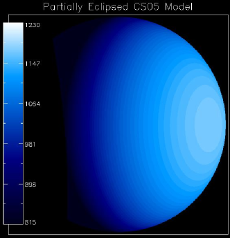
Figure 1: Partially eclipsed temperature maps in a CS05-like model of TrES-1 (left) and a Cho03-like model of HD189733b (right). The color-temperature scale (in K) is shown on the left of each panel. Notice how the different system geometries affect the orientation and shape of the eclipsing stellar limb, and consequently the detailed shape of the ingress/egress curves.

This is a parameterization of the atmospheric model of Cooper & Showman (2005), in which a hot spot is shifted by $\sim$60^o in longitude downstream of the sub-stellar point. For the hot spot itself, we adopt the same functional form as in the RadEq model above, except that the hottest region is only $\sim$400K hotter than the cold “night-side” (and shifted away from the sub-stellar point by 60^o in longitude). The left panel in Figure 1 shows the corresponding temperature map partially eclipsed.

Cho03-like Model:

This is a snapshot temperature map taken from one of the atmospheric models of Cho et al. (2003) and Cho et al. (2006) for HD209458b. Two cold spots associated with circumpolar vortices rotate around the planet semi-periodically, with a period typically several times that of the planet itself. The specific shallow-layer model parameters in the simulation used here are: global wind speed $\bar{U}=400$ m s^-1 and relative amplitude of thermal forcing $\eta=0.2$ (for a full discussion of the parameter space see Cho et al., 2006). The cold spots are $\sim$10% cooler than the average atmospheric temperature. A fixed phase of the atmospheric temperature pattern has been chosen here for simplicity (it rotates around the planet with time), approximately in such a way that the greatest difference in ingress/egress lightcurve shape is achieved relative to the RadEq model lightcurve shape. The right panel in Figure 1 shows the corresponding temperature map partially eclipsed.

We expect these parameterized, physically-motivated models to cover a wide enough range of possibilities for us to be able to assess the level of photospheric details that can be probed via the corresponding ingress/egress lightcurves. In particular, in the order RadEq/CS05-like/Cho03-lik3/Uniform, these models constitute a sequence of increasing deviation from simple radiative equilibrium, towards photospheric temperature uniformity.

We use these photospheric emission models to simulate ingress/egress curves for the three, bright hot Jupiters with Spitzer eclipse measurements: HD189733b, HD209458b, and TrES-1. All the system parameters used in our analysis are listed in Table 1. The range of temperatures in each photospheric model is adjusted to appropriate values for each planet of interest, using that system’s parameters. From the above description of the RadEq and Uniform model, it is clear that we have assumed negligibly small albedos in all cases. We find that a change of Bond albedo from $0$ to $0.3$ (a range characteristic of most Solar System planets; de Pater & Lissauer, 2001) has little influence on our main results, considering other systematic effects present. For computational reasons, we set the value of $T_{\rm night}$ to $700$ K in all our models. Here again, we find that this choice is not crucial because very little of the night side is generally visible to a distant observer, given the tidally-locked eclipse geometries considered here.

From the detailed model of Cooper & Showman (2005), values of $T_{0}$ and $T_{\rm night}$ for HD209458b’s photosphere are approximated as 1450K and 1010K, respectively. In our CS05-like models for the two other hot Jupiter systems, these values are rescaled in linear proportion to the value of the “redistributed” equilibrium temperature of the planet of interest (that is $T_{p}=T_{*}\sqrt{R_{*}/2a}$ for zero albedo; see Table 1). In the detailed HD209458b model of Cho et al. (2003, 2006) used here, the hottest and coldest temperatures reached overall are approximately 1460K and 1230K, with an average temperature of 1390K. In our Cho03-like models for the two other hot Jupiter systems, these values are also rescaled in linear proportion to the value of the “redistributed” equilibrium temperature of the planet of interest.

The conversion from local photospheric temperature to emission contributed by each apparent area element of the planetary disk (see §3.1 for projection details) is performed in two different ways. In a set of blackbody emission models, a simple Planck function is used. In a second set of models, a grid of detailed atmospheric spectral models derived from plane-parallel calculations is used to evaluate the local emission for effective temperatures in the range 700-2000K. No temperatures outside of this range of validity for the spectral models were allowed in our photospheric emission models. The plane-parallel spectral models are essentially extensions of the cloudless models described in Seager et al. (2005). Contrary to more detailed calculations (e.g. Barman et al., 2005), we ignore the 2D geometry of the radiative transfer problem when we use these plane-parallel calculations and implicitly assume isotropic emission of each planetary surface element in our photospheric emission models.

Planetary limb darkening (or brightening) could in principle be important in hot Jupiter atmospheres. It is not included in our basic models given the very simple method adopted (which assumes a well-defined photospheric temperature field and an isotropic emission). To estimate the effect that strong limb darkening could have on our overall analysis, we have included an optional limb darkening function in our emission models which can be applied to any of the models under consideration. The functional form adopted for this strong limb darkening is chosen to correspond to a geometrical decrease of the emitted flux with the cosine of the angle away from the sub-observer point. (i.e. $F=F_{0}\cos(\phi)$, where $\phi$ is the angle away from the sub-observer point). Since our analysis relies on well-defined photospheric temperatures, we have implemented this in our “limb-darkened” models with a simple decrease of the photospheric temperature as $\cos^{1/4}(\phi)$, superimposed on the photospheric temperature field of any of the four emission models defined above.

Another systematic source of errors for hot Jupiter eclipse mapping studies could be related to finite eclipse timing uncertainties. Even for planets with measured orbital eccentricities consistent with zero, the presence of an as yet undetected perturbing companion could lead to significant timing variations from one eclipse to the next (Agol et al., 2005; Holman & Murray, 2005). Careful measurements of transit times before and after any secondary eclipse could be used to put stringent constraints on the magnitude of these timing uncertainties. A thorough exploration of timing variation uncertainties for eclipse diagnostics is beyond the scope of the present analysis. Here, to evaluate simply the magnitude of these effects, we consider in some of our models the effects of arbitrarily time-shifting lightcurves produced by two different photospheric emission models, in such a way as to bring the mid-eclipse values closer to each other. This makes efforts to distinguish the models more difficult, even though we are not formally fitting the eclipse center time in our analysis. In principle, the influence of a perturbing planet results in timing offsets which vary in amplitude from orbit to orbit. Here we are only considering the simple consequences of a constant, detrimental temporal shift in our models. Although Agol et al. (2005) have shown that a wide range of timing variations are possible in general (from seconds to minutes and more), we will focus here on a representative value of 7 seconds for definiteness, on the assumption that careful transit monitoring could plausibly constrain secondary eclipse timing uncertainties to $\;\hbox to0.0pt{\lower 2.5pt\hbox{$\sim$}\hss}\raise 1.5pt\hbox{$<$}\;10$ seconds in any given system (which is about an order of magnitude improvement over current timing accuracies; e.g. Deming et al., 2006).

3 The Method

It is clear that current Spitzer data for a single eclipse in any of the three systems studied here do not contain enough information to determine the shape of the ingress or egress lightcurves with much accuracy (e.g. Deming et al., 2006). Multiple Spitzer eclipse observations would be required to derive meaningful constraints on the day-side photospheric emission properties of these hot Jupiters. The ability to distinguish between various photospheric emission models must then depend on whether or not the number of repeated observations needed is prohibitively large. To evaluate this, we simulate eclipse light curves produced by different photospheric emission models, add noise in proportion to known measurement errors and statistically determine the number of observations needed to differentiate between two specific models. In other words, our analysis provides a model-dependent estimate of the level of atmospheric details that can be probed with repeated ingress/egress measurements.

3.1 Simulating Eclipses

To simulate eclipse light curves, a photospheric temperature model for the planet is orthographically projected onto a disk, which is then eclipsed using the known geometry of the system. At each point in time during ingress or egress, the emission from non-eclipsed regions on the planetary disk is integrated, in proportion to the (apparent) area of each visible disk surface element. Two analyzes are performed simultaneously. One focuses simply on the bolometric emission under the assumption that each surface element emits like a blackbody at the corresponding photospheric temperature. The other analysis is spectral: the contribution to the monochromatic flux at Earth is calculated for each apparent surface element by using the local photospheric temperature to interpolate in the above-mentioned grid of plane-parallel spectral emission models. Spectral contributions are then integrated over specific Spitzer response curves, or the wavelength ranges of the future JWST NIRSpec gratings, to determine the amount of light that would be collected by these instruments. The spectral models used are subject to strong systematic effects in specific spectral regions (e.g. flux peak at $\sim 4$µm, as seen Fig 1 of Seager et al., 2005). Testing how strongly our main results depend on such systematic spectral features is the reason why we use an alternative, very idealized bolometric blackbody emission model in some of our eclipse simulations.

A 2D polar grid is constructed to describe the projected planetary disk, with 1000 radii sampled between 0 and $R_{p}$ (the planetary radius) and 1500 polar angles sampled between 0 and 2$\pi$. The radial resolution also determines the temporal resolution of our simulated eclipse curves since the stellar limb moves across the disk at a constant horizontal rate. We account for the curvature of the stellar limb, assuming it to be a perfectly opaque disk. We have tested our eclipse simulation apparatus by comparing results to the analytical solution described in Warner et al. (1971). With a [$r$,$\theta$] resolution of [1000,1500], a comparison to the analytical lightcurve solution for a straight stellar limb gives agreement at better than the 1% level (with growing errors towards the very end/beginning of ingress/egress because of grid under-sampling). The same level of accuracy is achieved in the case of a spherically curved stellar limb.

In our analysis, we account for the influence of each system’s specific geometry (i.e. inclination, ratio of planet and stellar radii, semi-major axis) on details of how the planetary disk is being eclipsed. Table 1 lists the geometrical parameters adopted for the three systems of interest. The orbital velocity is calculated as $v=2\pi a/P$, where $a$ is the planet’s orbital semi-major axis and $P$ is the corresponding orbital period. The vertical offset (from the observer’s point of view) between the centers of the planetary and stellar disks, $h$, is calculated as $h=a\sin(90^{\mathrm{o}}-i)$, where $i$ is the orbital inclination. The duration of ingress/egress is $t_{\rm gress}=(\sqrt{(R_{*}+R_{p})^{2}-h^{2}}-\sqrt{(R_{*}-R_{p})^{2}-h^{2}})/v$, where $R_{*}$ is the stellar radius. Figure 1 illustrates the eclipsing geometries for the TrES-1 and HD189733 systems. For simplicity, we ignore the effects of the small planetary rotational offset occurring between ingress and egress and consider instead that the sub-stellar point remains directly aligned towards the observer in all the models. The actual shift between ingress and egress is $\sim 10$^o for the three systems of interest. We have performed explicit tests and found that such a small rotational offset of the photospheric emission model generally has little effect on our main results, as compared to other more important sources of uncertainty.

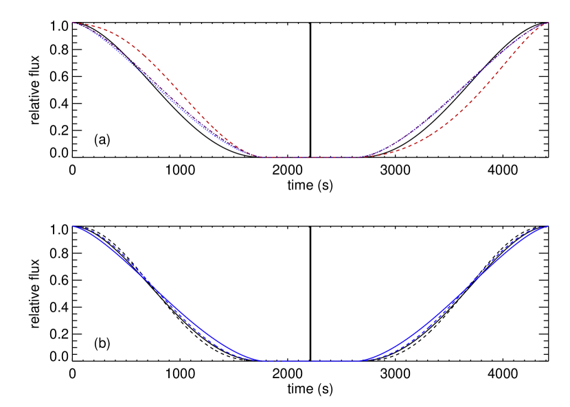
Figure 2: Simulated ingress and egress curves for different photospheric emission models of HD189733b: (a) RadEq model (black), Uniform model (dotted blue), CS05-like model (dashed red), and Cho03-like model (dot-dashed purple); (b) RadEq model (black), Uniform model (blue), RadEq model with strong limb darkening (dashed black), and Uniform model with strong limb darkening (dashed blue). Our analysis considers only the ingress and egress phases (separated by the vertical line) and thus excludes the full occultation period.

As an example, Figure 2 shows the bolometric blackbody ingress and egress light curves obtained in the case of HD189733b for each of the photospheric emission models considered in our analysis. Dashed lines highlight the effects that strong planetary limb darkening has on the RadEq and Uniform models. It is obvious from these curves that the differences between the various photospheric emission models under consideration are subtle. It is also important to realize the existence of some level of degeneracy in our models. For example, during egress (only), there is little difference between the curves predicted by the Cho03-like and the Uniform models because the stellar limb exposes the Cho03-like photospheric emission features in such a way that contributions from hot and cold regions more or less cancel out. Finally, let us emphasize that the various photospheric emission models introduced above only define the shapes of ingress/egress lightcurves, in units of relative flux, in our modeling strategy. An absolute flux unit common to all these models is effectively selected only when a noise magnitude is chosen to generate a system- and instrument-specific stream of simulated data, as we shall now describe.

3.2 Statistical Analysis

With simulated ingress/egress light curves in hand, we can use known or estimated measurement errors to simulate noisy eclipse data. From these simulations, we can statistically determine how much data is needed to differentiate between two specific photospheric emission models. For ease of comparison and definiteness, we chose the model without any heat redistribution, that is the RadEq model, to be our reference model. We generate an incrementally increasing amount of simulated eclipse data for this model and determine when it is that model lightcurves produced for other photospheric emission models become inconsistent with the accumulated stream of data (i.e. as a function of the number of repeated eclipse measurements). Our choice of the RadEq model as a reference is arbitrary, in the sense that any other model could be used as a reference for our statistical analysis. Notice, however, that by ruling out another model against the RadEq one, one effectively rules out some level of heat redistribution in the atmosphere studied. While any combination of two photospheric emission models could in principle be compared against each other, the interest of doing so is limited by the fact that all comparisons remain necessarily model-dependent. In the end, with our analysis we are only trying to assess the level of photospheric detail that could be distinguished by actual measurements. We will later suggest that non-parametric methods be considered for the study of hot Jupiter eclipses in the future.

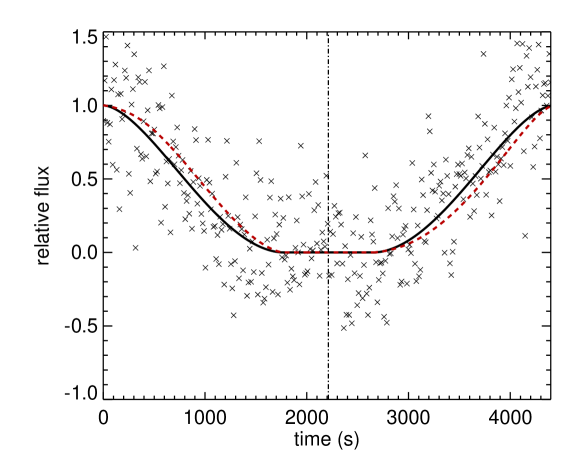
Figure 3: Example of ingress/egress simulated data for HD189733b in Spitzer’s 8µm IRAC band, for single-measurement noise of variance $\sigma_{1}=0.31$ (crosses) based on existing Spitzer measurements. For comparison, two noise-free curves are shown for the RadEq model (black) and CS05-like model (red dashed). Here again, our analysis excludes the full occultation period.

Throughout this analysis we work in units of relative flux. The planetary flux is normalized to its full day-side value, i.e. the value right before entering secondary eclipse (neglecting small rotational effects). A simulated data stream is generated on the basis of a cadence of observation and a Gaussian noise single-measurement error of variance $\sigma_{1}$ (in units of relative flux). The values of $\sigma_{1}$ adopted, as well as the cadence used to calculate the number of measurements occurring during one ingress or egress period, are estimated from previous measurements or simple extrapolations, as described in Section 3.3 for Spitzer, and Section 5.1 for JWST. Figure 3 shows an example of such a simulated data stream for HD189733b in one of Spitzer’s IRAC bands. Noiseless ingress/egress curves for two photospheric emission models (including the RadEq one used to generate the simulated noisy data) are over-plotted for comparison. Again, it is clear that repeated eclipses will be needed in this case if one wishes to discriminate between the two models, given with the level of noise in the data.

The quality of any photospheric emission model in fitting a set of simulated data is evaluated by calculating the reduced $\chi^{2}$ value for that model compared to the data. Since we are creating the simulated data from the reference RadEq model, with a sufficient number of repeated eclipse measurements, any other emission model will eventually provide a poor fit to the data (as measured by the reduced $\chi^{2}$ value). The process of simulating data is repeated, as needed, for an increasing number of eclipses, $N$, with identical error properties but a random temporal offset added to each new eclipse set. This offset is added to account for the likely lack of accurate phasing even between successive eclipses in a real data set. For each value $N$ of the number of accumulated eclipses, reduced $\chi^{2}$ values are calculated comparing any photospheric emission model of interest to the data until, after enough measurements, models (different from the RadEq one) are ruled out at the 99% confidence level by the accumulated data set.

Figure 4 illustrates this procedure. At each $N$, all models of interest are compared to the same set of simulated data, so that the random fluctuations in the data set affect all of the reduced $\chi^{2}$ values in a similar way, as is apparent in the fluctuation pattern common to each reduced $\chi^{2}$ curve. The value of $N$ at which a reduced $\chi^{2}$ line crosses the 99% confidence level and does not return below it, $N_{0}$, is our measure of the number of eclipses needed to reliably differentiate between that model and the reference RadEq model. For example, Figure 4 shows that the RadEq model can be differentiated from the CS05-like model with approximately 15 eclipses, since the latter is then ruled out according to our criterion. When a detrimental 7-second timing offset is added in the CS05-like model (in such a way that it makes harder to differentiate against the RadEq model), a total of $\sim$30 eclipses is required according to our criterion. A close inspection of Figure 4 suggests that this substantial difference could simply be a statistical fluke resulting from the use of one statistical realization of the data stream.

To account for statistical variations in the value of $N_{0}$ derived from single realizations of the data stream, we repeat the above procedure 500 times (i.e. we generate 500 data streams with identical parameters but different random number generators). From these 500 realizations, we obtain a representative distribution of $N_{0}$ values for a fixed set of model parameters. Figure 5 shows examples of such distributions of $N_{0}$ values for Spitzer measurements. From these distributions, we now see clearly that a 7-second detrimental offset in timing applied to the CS05-like model does indeed make it harder to differentiate that model from the reference RadEq model. To be able to distinguish the fiducial RadEq model from the CS05-like model in 96% of the data stream realizations, $39$ eclipses are needed. This number jumps to $52$ eclipses if the detrimental 7-second timing offset is imposed on the CS05-like model curve, thus showing that eclipse timing uncertainties do affect the eclipse diagnostics being discussed here

We note that other parametric methods, based on different eclipse diagnostics, exist. In particular, Williams et al. (2006) discuss the overall time shift between a Uniform model and an implementation of photospheric emission for the detailed atmospheric model of Cooper & Showman (2005). One advantage of our method over the time shift diagnostics is that we use more information, that is the full shape of the ingress/egress curves, which makes it less sensitive to degeneracies. To illustrate this point, we note that a comparable mid-eclipse time shift deviation from the prediction of the CS05-like model is expected for both the RadEq and the Uniform models, making it difficult to discriminate between these two models solely on the basis of a time shift (see Fig. 2). An adequately phased/rotated Cho03-like model could also induce a similar time shift relative to the RadEq and Uniform model predictions. Clearly, the issue of degeneracies is inherent to all parametric methods and we have already illustrated how our models also suffer from this limitation. In the future, non-parametric inversion techniques may thus be the best way to address this difficulty.

3.3 Estimating Spitzer Errors

So far, we have considered in detail only the specific case of HD189733b observed by Spitzer at 8µm with IRAC. The parameters used to produce the data stream in this case were inferred from actual observations of that system with Spitzer and from observations of another system with IRAC at 8µm. Specifically, the single-measurement error was taken to be $\sigma_{1}=0.31$ and 134 measurements were assumed to be collected per ingress/egress period. Here we describe how we estimate these two numbers for every possible combination of instrument and planetary system of interest. This necessarily involves some level of extrapolation since many such observations have not been performed (or reported) to date.

In the previous section, we defined $\sigma_{1}$ as the error per observational point, for unity eclipse depth (i.e. in our relative flux units). In absolute units, this corresponds to the single-measurement error divided by the eclipse depth flux-equivalent, which can both easily be obtained from previous Spitzer measurements when they exist. We have compiled the results of Deming et al. (2005) using MIPS on HD209458b, Charbonneau et al. (2005) using the 4.5 and 8µm IRAC bands on TrES-1 and Deming et al. (2006) using IRS on HD189733b. The values of $\sigma_{1}$ derived from these measurements are shown in bold in Table 2.

To estimate the errors for every possible combination of system and instrument, we pick an instrument, a specific spectral band, and rescale a known measurement error to derive the corresponding value for another system. Assuming that simple Gaussian noise statistics and the bright source limit are applicable, so that $\sigma_{F}=\sqrt{F}$, we expect the errors between system A and system B to scale approximately with the ratios of system fluxes as:

$$\frac{\sigma_{1,B}}{\sigma_{1,A}}\simeq\sqrt{\frac{F_{*,B}}{F_{*,A}}}\left[\frac{F_{p,A}}{F_{p,B}}\right]$$

where the $*$ and $p$ subscripts refer to the star and the planet, respectively. Using a simple blackbody-like scaling for the relative stellar and planetary fluxes, and isotropic emission in all cases, this expression becomes:

$$\frac{\sigma_{1,B}}{\sigma_{1,A}}\simeq\frac{d_{B}}{d_{A}}\left(\frac{R_{*,B}}{R_{*,A}}\right)\left(\frac{R_{p,A}}{R_{p,B}}\right)^{2}\sqrt{\frac{B_{\lambda}(T_{*,B})}{B_{\lambda}(T_{*,A})}}\left[\frac{B_{\lambda}(T_{p,A})}{B_{\lambda}(T_{p,B})}\right]$$ (1)

where $d$ is the distance to the system, $R$ is the object’s radius, $B_{\lambda}$ is the Planck function, $T$ is temperature, and $\lambda$ is taken to be the central wavelength of the instrumental band under consideration. The results of this extrapolation for $\sigma_{1}$ values are listed in Table 2.

Table 2 also lists in each case the number of single data point measurements per ingress/egress period. These values are calculated from the duration of ingress/egress for each planet, combined with the cadence of each instrument. The ingress/egress durations, $t_{\rm gress}$, are listed in Table 1. The cadences for existing measurements are 12.3 s for MIPS, 13.2 s for IRAC, and 14.7 s for IRS. New observing plans could result in different cadences, but these values should be sufficiently accurate at the level of detail of our analysis. We estimate that uncertainties in extrapolated $\sigma_{1}$ values may affect our results much more significantly.

4 Results for Spitzer

We performed an extensive survey of the parameter space of our eclipse models for each planetary system and Spitzer instrument of interest. The results of this exploration are summarized in Table 3.

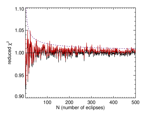
Figure 6: Example of the reduced $\chi^{2}$ values as a function of the number of eclipses, $N$, for data compared to the RadEq model (black) and the Uniform model (red) for HD189773b using Spitzer’s 8µm IRAC band. The models cannot be differentiated by this method.

Figure 6 shows a typical reduced $\chi^{2}$ test for what we estimate to be the best scenario for Spitzer, differentiating between the RadEq and Uniform models at 8µm with IRAC in the HD189733 system. Clearly, Spitzer is not sensitive enough to differentiate between these two models in any practical terms.

It is also impossible for Spitzer to differentiate the Cho03-like model from the RadEq model. One additional difficulty with the Cho03-like model is that the rotation of the temperature pattern would cause the detailed shape of the ingress/egress curves to change significantly over time if too many successive eclipses are required to reach good photometric accuracy. An instrument sensitive enough to differentiate the Cho03-like model from the RadEq model would probably have to do so in no more than a few successive eclipses to avoid excessive variations of ingress/egress shapes. In the specific Cho03-like model used here, the circumpolar vortices are $\sim$10% cooler than the average photospheric temperature. At the level of detail probed by Spitzer, we find that this model is indistinguishable from the Uniform model. (However, see Cho et al., 2006, for more extreme versions of this class of models.)

Of all the models we have considered in our survey, the only one that Spitzer could possibly distinguish from the RadEq reference model is the CS05-like model, in the bright HD189733 system. Even in this case, from 9 to 52 eclipses are required (see Table 3 and Figure 4). This would be a very expensive observing program considering the strongly model-dependent nature of the diagnostics involved.

If, instead of the spectral predictions of plane-parallel atmospheric calculations, we use simple, bolometric, blackbody photospheric emission models, we find in general that fewer eclipses are necessary to permit discrimination between two models (see comparisons in Table 3). Note that this difference is not due to the more efficient character of blackbody emission since all our ingress/egress models are eclipse-depth normalized in such a way that it is the normalized ingress/egress shape that is being used as a diagnostic. Rather, this shows that details of how the spectral energy distribution varies with local photospheric temperature do affect the diagnostics of our analysis. As additional observational constraints on hot Jupiter atmospheres become available, some classes of emission models (e.g. with or without clouds) will be favored over others. Nevertheless, the sensitivity of eclipse diagnostics to details of the spectral emission model assumed could remain significant. This is another important reason to favor diagnostics based on non-parametric inversion techniques in the future.

While limb darkening could worsen the $N_{0}$ statistics discussed so far, by reducing the information content of photospheric emission regions close to the planetary limb, we have not systematically explored this possibility in the context of Spitzer observations given the already poor statistics. We come back to this issue in the context of JWST observations below.

5 The Case For JWST

Since Spitzer will likely not be able to constrain photospheric temperatures and atmospheric models at a very meaningful level with eclipse mapping, we turn our attention to the upcoming James Webb Space Telescope (JWST). The much increased sensitivity of JWST results from a combination of larger collecting area and reduced background. Of the instruments currently planned for JWST, we chose to focus on NIRSpec for our comparative analysis. This instrument will have three spectral gratings, covering the range of wavelengths from 1-5µm. Spectra are not required for our analysis (or for eclipse mapping in general), but the dispersion of light provided by the gratings turns out to be useful in avoiding possible instrument saturation for the three bright systems of interest here. It may be possible to use the NIRCam instrument to study eclipses in dimmer systems than the three bright ones considered here, thus increasing the total number of potential target systems, but we have not explored this possibility in detail. Our goal here is a first, very preliminary assessment of JWST capabilities in terms of eclipse mapping, relative to the Spitzer case. We caution that it is difficult to estimate high-contrast measurement errors for an instrument that was not designed for that task.

5.1 Estimating JWST Measurement Errors

As the JWST design is not yet finalized, our estimate of measurement errors for NIRSpec is only approximate. We treat each NIRSpec spectral grating as a single bandpass, using the spectrally integrated light only. We base our estimates on the detailed analysis of Valenti et al. (2005) for a NIRSpec simulated (spectral) measurement of a secondary eclipse of HD209458b. The three gratings G140H, G235H, and G395H cover the wavelength ranges 1-1.8µm, 1.7-3µm, and 2.9-5µm, respectively. For HD209458b, the respective exposure times are estimated to be 2.4, 2.4, and 3.6 s. Adding a conservative estimate of 0.9 s for reset between exposures results in cadences of 3.3 and 4.5 s for G140H/G235H and G395H, respectively (Valenti et al., 2005).

A calculation of the single-measurement error, $\sigma_{1}$, entering our ingress/egress simulations is more complex and requires estimates of the number of stellar and planetary photons that would be detected by each grating during one exposure. Valenti et al. (2005) simulate noisy spectra for the HD209458 system, for two hours of exposure time. To estimate the eclipse depth in any given grating, we divide the planetary spectrum by the stellar spectrum and sum over the wavelength range of that grating. Since the spectra are summed over two hours of exposure time, the number of photons collected during one exposure is easily obtained from the number of single exposures in a two-hour period. We assume that the noise scales simply with the inverse square root of the number of detected stellar photons (like Valenti et al., 2005). The single-measurement error is then given by $\sigma_{1}=(\sqrt{N_{*}\times N_{\rm exp}})/(N_{p})$, where $N_{*}$ is the number of stellar photons, $N_{p}$ is the number of planetary photons and $N_{\rm exp}$ is the number of unit exposures. Using Figures 3 and 4 from Valenti et al. (2005), a spectral resolution $R=2700$ and a value of $N_{\rm exp}$ based on the cadences listed above, we deduce the approximate single-measurement errors for HD209458b listed in italics in Table 2. Using the same system-to-system scaling method as before (§ 3.3), we then extrapolate single-measurement $\sigma_{1}$ errors for HD189733b and TrES-1 (see Table 2).

As a consistency check on the $\sigma_{1}$ values thus derived from Valenti et al. (2005), the following simple arguments can also be used to scale values from the 4.5µm Spitzer-IRAC band to the 4µm JWST spectral gratings. Wavelength ranges for these two bands overlap, but they are not equivalent: the NIRSpec grating covers roughly 3-5µm, while the IRAC band covers approximately 4-5µm. The additional 3-4µm sub-range will allow JWST gratings to collect more photons and probe a region where the planet to star flux ratio is somewhat higher (due to the presence of a flux peak at  $\sim$$<$ 4µm; see Fig. 1 of Seager et al., 2005). Assuming that NIRSpec has 1000-fold increased sensitivity relative to IRAC, that the NIRSpec cadence is about three times that of IRAC, and that the JWST to Spitzer eclipse depth ratio in these bands is about a factor of two (from the 4µm flux peak), we estimate a Spitzer-to-JWST $\sigma_{1}$ ratio of $\sim$50. This is consistent with the ratio $58$ listed in Table 2. While this crude comparison lends support to the $\sigma_{1}$ values adopted below in our JWST analysis, there is clearly a need for better evaluations of the photometric accuracy expected with JWST for hot Jupiter eclipse mapping programs.

5.2 Results For JWST

The results of our survey of JWST/NIRSpec capabilities are summarized in Table 3. The much increased sensitivity allows relatively small photospheric emission features to be distinguished in the shapes of ingress/egress lightcurves in just one or a few eclipses. For HD189733b and HD209458b, the RadEq model would be easily distinguished from the Uniform and Cho03-like models by using the 4µm grating. HD189733b is bright enough that any of the gratings would in fact be very useful, while for HD209458b, the 4µm grating is a strongly preferable choice. The errors for this grating are expected to be significantly lower than the errors for the other two, partly because the planet to star flux ratio is higher at these wavelengths (according to the similar spectral models we and Valenti et al. 2005 used). A similar attempt to discriminate between the RadEq model and the Uniform model may require a prohibitively large number of eclipses for TrES-1. With the same 4µm grating, our results indicate that the CS05-like model can be differentiated from the RadEq one on all three planets. We also find this time that, given the much increased sensitivity of JWST, applying a detrimental 7 s timing offset to the CS05-like model has little consequence for attempts to differentiate that model from the RadEq one.

When we superimpose a strong limb darkening law on our Uniform photospheric emission model, it can be more difficult to differentiate that model from the RadEq model. As an example, observing HD189733b with the 4µm grating, one eclipse is still enough to differentiate between the RadEq model and the limb-darkened Uniform model, but five eclipses are required to do so with the 1.4µm grating. At the level of precision achievable with JWST, it will thus be important to self-consistently account for limb darkening effects for reliable eclipse diagnostics. This is yet one more reason to focus on non-parametric inversion techniques which, by construction, automatically incorporate any photospheric limb darkening present.

As in Section 4, we find that the simplified bolometric blackbody analysis generally leads to a reduction in the number of eclipses needed for model differentiation, relative to the analysis based on the detailed spectral emission models. We interpret this as indicating that emission in the spectral models vary generally less with temperature (in relevant narrow spectral bands) than the Planck function does bolometrically. We note that a counterexample of this general trend is found at the shortest wavelengths considered (the 1.4µm grating). For this grating, the range of photospheric temperatures on HD189733b conspires to make the emission properties in the spectral model vary more over ingress/egress than in the corresponding blackbody model. This time, a lower number of eclipses is needed to differentiate between the RadEq model and the Uniform model, according to spectral models. Altogether, comparisons between spectral and bolometric blackbody versions of our eclipse analysis, and their qualitative agreement, suggest that our main conclusions (in terms of the number of eclipses required for model differentiations) are not too strongly affected by systematic effects or uncertainties in the specific cloudless spectral emission models adopted throughout our analysis.

As a special case, we have also considered the possibility of differentiating between the Cho03-like and the Uniform photospheric emission models on HD189733b. We find that the 4µm NIRSpec grating should perform measurements precise enough to make the distinction between these two photospheric emission models possible with a single eclipse measurement (see the last three lines in Table 3). This would alleviate complications arising from temporal variations of the rotating atmospheric pattern, which are expected in Cho03-like atmospheric models. Let us recall that we have fixed the phase of the weather pattern in all our Cho03-like models to produce the greatest difference in ingress/egress shapes with respect to the RadEq model predictions. We selected a phase for the cold circumpolar vortices that would most easily be distinguished from that RadEq model. In a realistic situation, this specific phase would only be observed by chance coincidence. Our goal here was merely to determine the level of photospheric details that can be probed with JWST. This exercise shows that features of amplitudes and sizes similar to those of the circumpolar spots present in the Cho03-like model considered here (approximately 10% cooler than the average planetary photospheric temperature) are within the reach of JWST.

6 Summary and Conclusions

The shape of ingress and egress curves produced when a hot Jupiter is gradually eclipsed by its parent star contains detailed information on the planet’s photospheric emission properties. Hot Jupiter atmospheric modeling efforts would greatly benefit from this information if it were to become available through applications of eclipse mapping techniques. In an attempt to evaluate the feasibility of eclipse mapping for hot Jupiters, we have generated ingress/egress lightcurves expected for a variety of plausible photospheric emission models and asked whether these models could be differentiated from one another, on the basis of repeated eclipse measurements with current or future infrared facilities. We found that Spitzer has insufficient photometric accuracy to make efficient use of these eclipse diagnostics. Simple scalings indicate that a system at least ten times brighter than HD189733b, currently the brightest known eclipsing hot Jupiter, would be needed for Spitzer to yield meaningful results in this respect. On the other hand, our preliminary analysis suggests that JWST has the potential to reveal relatively subtle features at the photospheres of currently known eclipsing hot Jupiters.

Our analysis is voluntarily simple and limited in scope. By construction, we only compare specific photospheric emission models. This necessarily results in conclusions which are rather model-dependent. In addition, our treatment of atmospheric radiative transfer, and the related planet’s photospheric emission, was relatively simple. We assumed the existence of a well-defined photospheric surface in all our spectral models, we combined simple horizontal photospheric temperature maps with the results of 1D vertical radiative transfer calculations obtained independently and thus largely ignored important two- or three-dimensional geometrical effects in our analysis. Nevertheless, comparisons with crude bolometric blackbody emission models suggest that our main conclusions on the feasibility of using eclipse diagnostics with Spitzer and JWST are not too strongly affected by our various model specifics or shortcomings, because they mostly depend on the photometric accuracy achievable for the ingress/egress portions of infrared secondary eclipses.

Throughout our analysis, we stressed the advantages of non-parametric inversion methods for eclipse mapping, which would offer model-independent constraints on the photospheric emission properties of eclipsing hot Jupiters. By combining data at different wavelengths, and thus probing photospheres at different heights, 3-dimensional emission maps of hot Jupiter atmospheres could potentially be obtained. It remains to be seen with what precision this concept can be applied in practice. It is likely that our model-dependent analysis overestimates the level of details that can be probed by JWST with non-parametric eclipse mapping methods, but the promising nature of results obtained so far and the large potential value for the exoplanet science community provide strong motivations for a more careful assessment of this exciting new possibility.

Table 1: System parameters adopted

	HD189733	HD209458	TrES-1
distance (pc)	19	47	150
R∗ (R⊙)	0.76	1.146	0.83
T∗ (K)	5050	6000	5250
Rp (RJup)	1.26	1.35	1.04
Tp (K)	1200	1440	1160
semi-major axis, $a$ (AU)	0.0313	0.046	0.0394
orbital period, $P$ (days)	2.219	3.524	3.030
orbital velocity, $v$ (km s-1)	154	142	142
orbital inclination, $i$ (o )	85.3	87.1	89.5
star-planet offset, $h$ (Rp)	4.28	3.62	0.69
ingress/egress $t_{\rm gress}$ (s)	1770	1520	1050

References. — ^aPerryman et al. (1997), ^bAlonso et al. (2004), ^cBouchy et al. (2005), ^dBrown et al. (2001), ^eSozzetti et al. (2004), ^fMazeh et al. (2000), ^gCharbonneau et al. (2000)

Table 2: JWST and Spitzer single-measurement errors, $\sigma_{1}$, and numbers of measurements, $N_{1}$, during a full ingress/egress

Instrument,	HD189733b	HD209458b	TrES-1
wavelength (µm)	$\sigma_{1}$, $N_{1}$	$\sigma_{1}$, $N_{1}$	$\sigma_{1}$, $N_{1}$
JWST, G140H, 1.4	1.5, 536	1.4, 461	26, 318
JWST, G235H, 2.3	0.3, 536	0.4, 461	4, 318
JWST, G395H, 4	0.02, 393	0.04, 338	0.3, 233
Spitzer, IRAC, 4.5	0.29, 134	0.64, 115	4.1, 80
Spitzer, IRAC, 8	0.27, 134	0.71, 115	3.8, 80
Spitzer, IRS, 16	0.46, 120	1.3, 103	6.2, 71
Spitzer, MIPS, 24	1.2, 144	3.5, 124	17, 85

Note. — Values in bold are calculated from previous measurements and values in italics are calculated from the estimates of Valenti et al. (2005). All other values were scaled accordingly (as described in Section 3.3).

Table 3: Number of eclipses needed to differentiate between emission models with Spitzer or JWST.

System	Instrument, wavelength (µm)	Models compared	Neclipses
Spitzer
any system	any wavelength	RadEq, Uniform	$>$500
HD189733	IRAC, 8	RadEq, CS05 w/no timing uncert.	39 (78)
HD189733	bolometric w/8µm noise stats.	RadEq, CS05 w/no timing uncert.	9 (18)
HD189733	IRAC, 8	RadEq, CS05 w/7s timing uncert.	52 (104)
HD189733	bolometric w/8µm noise stats.	RadEq, CS05 w/7s timing uncert.	10 (21)
JWST
TrES-1	NIRSpec, any grating	RadEq, Uniform	$>$500
HD209458	NIRSpec, 1.4 or 2.3	RadEq, Uniform	$>$500
HD209458	NIRSpec, 4	RadEq, Uniform	2
HD209458	bolometric w/4µm noise stats.	RadEq, Uniform	1
HD209458	NIRSpec, 1.4	RadEq, CS05 w/7s or w/no timing uncert.	$>$450
HD209458	NIRSpec, 2.3	RadEq, CS05 w/7s or w/no timing uncert.	3
HD209458	NIRSpec, 4	RadEq, CS05 w/7s or w/no timing uncert.	1
HD189733	NIRSpec, 1.4	RadEq, any model	$>$500
HD189733	NIRSpec, 2.3	RadEq, Uniform	$>$300
HD189733	NIRSpec, 2.3	RadEq, CS05 w/7s or w/no timing uncert.	2 (5)
HD189733	bolometric w/2.3µm noise stats.	RadEq, CS05	3 (11)
HD189733	NIRSpec, 4	RadEq, any model	1 (1)
HD189733	NIRSpec, 4	RadEq, Uniform w/ld	1 (1)
HD189733	NIRSpec, 4	Uniform, Cho03	2 (2)
HD189733	bolometric w/4µm noise stats.	RadEq, any model	1 (1)
HD189733	bolometric w/4µm noise stats.	Uniform, Cho03	1 (1)

Appendix A Revised HD189733b Radius

Recently, Bakos et al. (2006) and Winn et al. (2007) have revised the value of the radius of HD189733b downward from $1.26$ to $1.15$ Jupiter radii. Accordingly, we have reconsidered our eclipse lightcurve analysis for this planet. The revised number of eclipses needed to differentiate between various photospheric emission models appears in parenthesis in Table 3. The smaller radius results in increased photometric errors and thus an increased number of required eclipses. Nonetheless, we find that the photometric accuracy of JWST at 4µm remains good enough for one or two eclipses to distinguish reliably among the various emission models considered.

Figure 4: Reduced $\chi^{2}$ values of three different model fits to a simulated dataset for HD189733b, as a function of the number of repeated eclipse measurements, $N$. The single-measurement noise variance adopted in the simulated ingress/egress dataset is $\sigma_{1}=0.31$. The 99% confidence limit above which models are ruled out is shown as a dashed line. The RadEq model used to generate the simulated ingress/egress dataset is shown as a black line. With a large enough set of eclipse data, other models (red line: CS05-like model; blue line: CS05-like model with detrimental 7 second timing offset) are eventually ruled out at high significance.

Figure 5: Histograms of $N_{0}$, the number of eclipses needed to differentiate at the $99\%$ confidence level between fits to the correct underlying RadEq model and a CS05-like model (a), or a CS05-like model with an imposed 7 second detrimental timing offset (b). These distributions emerge from 500 independent realizations of repeated eclipse sequences like the one shown in Figure 4. $N_{0}$ is defined as the value of $N$ in such sequences at which each model’s reduced $\chi^{2}$ curve reliably crosses the 99% confidence level.

References

- Agol et al. (2005) Agol, E., Steffen, J., Sari, R., & Clarkson, W. 2005, MNRAS, 359, 567
- Alonso et al. (2004) Alonso, R., et al. 2004, ApJ, 613, L153
- Baptista (2001) Baptista, R. 2001, in Astrotomography, Indirect Imaging Methods in Observational Astronomy, Eds H.M.J. Boffin, D. Steeghs and J. Cuypers, Lecture Notes in Physics, vol. 573, p.307
- Bakos et al. (2006) Bakos, G. A. et al. 2006, ApJ, 650, 1160
- Barman et al. (2005) Barman, T. S., Hauschildt, P. H., & Allard, F. 2005, ApJ, 632, 1132
- Bobinger (2000) Bobinger, A. 2000, A&A, 357, 1170
- Bouchy et al. (2005) Bouchy, F., et al. 2005, A&A, 444, L15
- Brown et al. (2001) Brown, T. M., Charbonneau, D., Gilliland, R. L., Noyes, R. W., & Burrows, A. 2001, ApJ, 552, 699
- Burkert et al. (2005) Burkert, A., Lin, D. N. C., Bodenheimer, P. H., Jones, C. A., & Yorke, H. W. 2005, ApJ, 618, 512
- Burrows et al. (2005) Burrows, A., Hubeny, I., & Sudarsky, D. 2005, ApJ, 625, L135
- Burrows et al. (2006) Burrows, A., Sudarsky, D., & Hubeny, I. 2006, ApJ, 650, 1140
- Butler et al. (2006) Butler, R. P. et al. 2006, ApJ, 646, 505
- Charbonneau et al. (2005) Charbonneau, D., et al. 2005, ApJ, 626, 523
- Charbonneau et al. (2000) Charbonneau, D., Brown, T. M., Latham, D. W., & Mayor, M. 2000, ApJ, 529, L45
- Cho et al. (2003) Cho, J. Y-K., Menou, K., Hansen, B. M. S., & Seager, S. 2003, ApJ, 587, L117
- Cho et al. (2006) Cho, J. Y-K., Menou, K., Hansen, B., & Seager, S. 2006, ApJ submitted, astro-ph/0607338
- Cooper & Showman (2005) Cooper, C. S., & Showman, A. P. 2005, ApJ, 629, L45
- de Pater & Lissauer (2001) de Pater, I., & Lissauer, J. 2001, Planetary Sciences, by Imke de Pater and Jack Lissauer. Cambridge University Press, 2001, 544 pp.
- Deming et al. (2006) Deming, D., Harrington, J., Seager, S., & Richardson, L. J. 2006, ApJ, 644, 560
- Deming et al. (2005) Deming, D., Seager, S., Richardson, L. J., & Harrington, J. 2005, Nature, 434, 740
- Harrington et al. (2006) Harrington, J. et al. 2006, Science, 314, 623
- Holman & Murray (2005) Holman, M. J. & Murray, N. W. 2005, Science, 307, 1288
- Horne (1985) Horne, K. 1985, MNRAS, 213, 129
- Iro et al. (2005) Iro, N., Bezard, B. & Guillot, T 2005, A&A, 436, 719
- Fortney et al. (2005) Fortney, J. J., Marley, M. S., Lodders, K., Saumon, D., & Freedman, R. 2005, ApJ, 627, L69
- Fortney et al. (2006) Fortney, J. J., Cooper, C. S., Showman, A. P., Marley, M. S.& Freedman, R. 2006, ApJ in press, astro-ph/0608235
- Lubow et al. (1997) Lubow, S. H., Tout, C. A., & Livio, M. 1997, ApJ, 484, 866
- Mazeh et al. (2000) Mazeh, T., et al. 2000, ApJ, 532, L55
- Menou et al. (2003) Menou, K. Cho, J. Y.-K., Seager, S. & Hansen, B. M. S. 2003, ApJ, 587, L113
- Ogilvie & Lin (2004) Ogilvie, G. I., & Lin, D. N. C. 2004, ApJ, 610, 477
- Perryman et al. (1997) Perryman, M. A. C., et al. 1997, A&A, 323, L49
- Rasio et al. (1996) Rasio, F. A., Tout, C. A., Lubow, S. H., & Livio, M. 1996, ApJ, 470, 1187
- Rutten (1996) Rutten, R. C. M. 1996, in proceedings of the 176th Symposium no. 176 of the International Astronomical Union, Eds Klaus G. Strassmeier and Jeffrey L. Linsky, Kluwer Academic Publishers, Dordrecht, p.69
- Rutten (1998) Rutten, R. C. M. 1998, A&AS, 127, 581
- Seager et al. (2005) Seager, S., Richardson, L. J., Hansen, B. M. S., Menou, K., Cho, J. Y.-K., & Deming, D. 2005, ApJ, 632, 1122
- Showman & Guillot (2002) Showman, A. P. & Guillot, T. 2002, A&A, 385, 166
- Sozzetti et al. (2004) Sozzetti, A., et al. 2004, ApJ, 616, L167
- Spruit (1994) Spruit, H. C. 1994, A&A, 289, 441
- Stern (1992) Stern, S. A. 1992, ARA&A, 30, 185
- Valenti et al. (2005) Valenti, J. A., et al. 2005, BAAS, 37, 1350
- Warner et al. (1971) Warner, B., Robinson, E. L., & Nather, R. E. 1971, MNRAS, 154, 455
- Williams et al. (2006) Williams, P. K. G., Charbonneau, D., Cooper, C. S., Showman, A. P., & Fortney, J. J. 2006, ApJ, 649, 1020
- Winn et al. (2007) Winn, J. N. et al. 2007, AJ, 133, 1828