Metal Absorption Profiles from the Central Star of the Planetary Nebula M27 (NGC 6853, PN G060.8-03.6, the Dumbbell) – Photospheric and Nebular Line Identifications

Abstract

High resolution spectra of the hot central star of the planetary nebula (CSPN) M27, acquired with the Far Ultraviolet Spectroscopic Explorer (FUSE), have revealed an unusually rich set of narrow molecular hydrogen absorption features. This object is also unique in that the velocity of nebular absorption features are cleanly separated from the velocity of the intervening interstellar medium. These features blend with and in many cases obscure atomic features. We have developed a continuum model of the CSPN including atomic and molecular hydrogen absorption. Using this model we have identified and tabulated the metal lines as arising from either photospheric, nebular and/or non-nebular velocity systems. We find the nebular outflow and ionization balance to be stratified with high ionization states favored at low velocity and low ionization states favored at high velocity. Neutrals and molecules are found at a velocity that marks the transistion between these two regimes. These observations are a challenge to the interacting wind model of PN evolution. Mappings at high resolution of the line profiles for C I - IV, N I - III, O I, O VI, Si II - IV, P II - V, S II - IV, Ar I - II and Fe II - III within the FUSE and STIS bandpasses are presented. The digitial spectra of the star and the model are freely available on the H₂ools website. They will be useful for photospheric analyses seeking to determine the metallicity of the central star and for absorption line based atomic and molecular abundance determination of the nebular outflow.

1. Introduction

High resolution spectra of the hot central star (CS) of the Planetary Nebula (PN) M27 (NGC 6853, PN G060.8-03.6, the Dumbbell), acquired with the Far Ultraviolet Spectroscopic Explorer (FUSE), have revealed an unusually rich set of narrow molecular hydrogen absorption features, spanning the entire bandpass. FUSE carriers no on-board source for wavelength calibrations and consequently M27 has been observed numerous times for this purpose, producing in the process a high quality data set as illustrated in Figure 1. The high density of the molecular lines presents problems for the identification and analysis of atomic features arising from the stellar photosphere and interstellar medium (ISM).

In a separate work (McCandliss et al., 2007, hereafter Paper I) we have developed a molecular and atomic hydrogen absorption model that, when applied to a readily available pure hydrogen helium hot white dwarf model of the CS (Rauch, 2003), provides a reasonable template against which the atomic absorption features from other metal line systems can be isolated. Here we compare the model to the observations and present a list of line identifications for atomic species associated with the stellar photosphere, the surrounding nebula and non-nebular ISM. We also present high resolution absorption line profiles from STIS and FUSE for the metals C I - IV, N I - III, O I, O VI, Si II - IV, P II - V, S II - IV, Ar I - II and Fe II - III.

Table 1FUSE Observation Summary

Observation	Date	APER	EXP:LiF1a	EXP:SiC1b	EXP:LiF2a	EXP:SiC2a
			(ksec)	(ksec)	(ksec)	(ksec)
M1070301	2000-09-03	MDRS	15.5	8.0	15.6	8.9
M1070302	2000-09-24	HIRS	17.5	4.8	13.3	5.6
M1070303	2001-05-28	LWRS	7.4	7.5	7.3	7.0
M1070304	2001-05-29	MDRS	7.0	4.8	6.6	0.6
M1070305	2001-05-29	HIRS	8.0	4.1	6.3	2.0
M1070306	2001-07-28	LWRS	7.1	7.1	7.2	7.1
M1070307	2001-07-28	MDRS	6.7	3.5	6.5	5.1
M1070308	2001-07-29	HIRS	8.5	3.4	6.3	3.3
M1070309	2001-08-01	LWRS	7.5	7.6	7.7	7.4
M1070310	2001-08-01	MDRS	6.6	4.1	6.4	4.8
M1070311	2001-08-01	HIRS	7.8	0.6	5.6	0.8
M1070312	2002-10-30	LWRS	5.0	5.1	4.8	5.0
M1070313	2002-10-30	MDRS	7.0	3.3	6.4	3.0
M1070314	2002-11-02	HIRS	3.3	0.9	2.4	0.7
M1070315	2004-05-25	LWRS	5.3	5.3	4.3	4.4
M1070316	2004-05-25	MDRS	4.0	2.9	4.9	4.4
M1070317	2004-05-25	HIRS	6.5	3.2	5.0	4.3
M1070319	2002-11-03	HIRS	2.7	1.1	2.0	0.9
P1043301	2000-06-05	LWRS	16.9	16.5	16.3	16.9

Paper I finds the observed atomic and molecular velocity stratification in the nebular outflow of M27 is challenging to explain in the context of the standard interacting winds model for PNe (Kwok et al., 1978). A similar challenge has been made by Meaburn (2005) (see also Meaburn et al., 2005a, b) who used high resolution position-and-velocity spectroscopy of the optical emission lines to derive the ionization kinematics of several objects. They find that ballistic ejection could have been more important than interacting winds in shaping the dynamics of PNe. In the interacting winds model a high speed ($\sim$ 1000 km s^-1) highly ionized radiation driven wind from the hot star shocks and ionizes a slow moving ($\sim$ 10 km s^-1), high density mostly molecular asymptotic giant branch (AGB) wind. In Paper I no evidence was found for a high speed radiation driven wind. The upper limit to the terminal expansion velocity is $\approx$ 70 km s^-1. The atomic line profiles show that high ionization material appears at low velocities ($\lesssim$ 33 km s^-1) and low ionization material appears at high velocities (33 – 65 km s^-1). At the transition velocity (33 km s^-1) between these two regimes, a predominately neutral atomic medium appears along with the vibrationally excited H₂. The molecular abudance in the nebula is low ($N(\mbox{H${}_{2}$})$/$N($H I) $\ll$ 1).

The Paper I study found that, despite the close proximity of a hot central star, the molecular hydrogen ro-vibration levels of the ground state were close to thermal ($\sim$ 2000 K). They found no detectable levels of far-UV fluorescence of molecular hydrogen, although Ly$\alpha$ pumped fluorescence has been detected by Lupu et al. (2006). Surprisingly, they also found that the line-of-sight was devoid of dust. The temperature implied by the molecular hydrogen suggests that the diffuse nebular medium is too hot for dust to form. They argue that the clumpy medium seen in the CO map of Bachiller et al. (2000), which cast the [O III] shadows seen by Meaburn & Lopez (1993) and O’Dell et al. (2002), are the source of the excited molecular hydrogen for the diffuse nebular medium and may harbor depleted material (dust). A depletion analysis of the Fe, Si, and S in the nebular outflow could provide information as to whether these clumps are composed of depleted material that is being released into the diffuse medium along with the molecular hydrogen.

The digitial spectra used in this study, are available at the following url,
http://www.pha.jhu.edu/~stephan/H2ools/M27kruk04/.
This dataset will be useful for photospheric analyses of the central star and for studies seeking to understand the kinematics of the atomic and molecular abundances in the nebular outflow.

Figure 1.— Signal-to-noise ratio of the eight coadded spectral segments taken through the HIRS spectrograph aperture. The individual segments are labeled.

2. Datasets

2.1. FUSE

FUSE spectra of the CS (MAST object ID GCRV12336) were acquired under the observatory wavelength calibration program (ID: M107). The CS was observed numerous times through all three focal-plane apertures: large (30″)², medium (20″$\times$ 4″) and small (20″$\times$ 1.25″); referred to respectively as LWRS, MDRS, and HIRS. A summary of the observations is given in Table 1. All spectra were acquired in TTAG mode. Each observation was performed as a series of exposures, ranging in length from 0.5 ksec to 3 ksec. Each exposure produces 8 individual spectra; one from each of two detector segments for each of the 4 optical channels. Effective exposure times are listed in the table for the more interesting segment in each channel. Exposure times occasionally differ slightly from one segment to another because the detector high voltage in a given segment can be reduced temporarily in response to event bursts or brief current spikes. Exposure times also differ from one channel to another as a result of channel misalignment effects. For a description of the detectors, channel alignment issues, systems nomenclature and other aspects of the FUSE instrument, see Moos et al. (2000) and Sahnow et al. (2000).

The exposures were processed with the following procedure. The raw data were calibrated using Calfuse 3.0.7. The resulting spectra for a given aperture (LWRS, MDRS or HIRS) were screened to identify the peak detected stellar flux. Exposures with less than 40% of the peak flux (a small fraction) were discarded. The remaining were normalized to the peak flux, yielding an effective exposure time. Channel/segments were coaligned with a cross-correlation procedure on narrow ISM lines. Spectra were shifted by whole pixel units to avoid smoothing and combined by effective exposure time weighted average. At this point there is one spectrum for each spectrograph aperture, divided among the 8 channel/segment combinations. The MDRS spectra were put on an absolute wavelength scale by adjusting each channel/segment spectrum so that the H₂ lines arising from the hot component of the molecular gas are at a fiducial offset (–69 km s^-1, see § 4.1 regarding this point). Finally, the normalization of the MDRS and HIRS were readjusted to match that of the LWRS and the zero point offsets of the HIRS and LWRS channel/segment were adjusted to match the MDRS. We use the HIRS data in this work as it yields the highest resolution.

Each extracted segment has associated with it a set of one dimensional arrays: wavelength (Å), flux (ergs cm^-2 s^-1 Å^-1), and estimated statistical error (in flux units). Figure 1 shows the signal-to-noise and spectral range for each of the coadded HIRS segments, obtained by dividing a flux array by the corresponding statistical error array. The signal-to-noise estimated in this way is purely statistical and does not account for systemic errors, such as detector fixed pattern noise. In the low sensitivity SiC channels the continuum signal-to-noise ranges between 10 – 25, while in the higher sensitivity LiF channels it is 20 – 55. The resolution of the coadded spectra changes slightly as a function of wavelength for each segment. In modeling the molecular hydrogen absorption, we find that a gaussian convolution kernel with a full with at half maximum of 0.05 Å at 1000 Å (spectral resolution $R$ = 18,000, velocity resolution ${\delta}V$ $\approx$ 17 km s^-1) provides a good match to the unresolved absorption features throughout much of the bandpass.

Close comparison of the wavelength registration for overlapping segments reveals isolated regions, a few Å in length, of slight spectral mismatch ($\sim$ a fraction of a resolution element) in the wavelength solutions. Consequently, combining all the spectra into one master spectrum will result in a loss of resolution. However, treating each channel/segment individually increases the bookkeeping associated with the data analysis. Further, because fixed pattern noise tends to dominate when the signal-to-noise is high, there is little additional information to be gained in analyzing a low signal-to-noise data set when high signal-to-noise is available. For these reasons we elected to form two spectra each of which covers the 900 – 1190 bandpass contiguously, using the following procedure. The flux and error arrays for the LiF1a and LiF1b segments were interpolated onto a common linear wavelength scale with a 0.013 Å bin, covering 900 – 1190 Å. The empty wavelength regions, being most of the short wavelength region from 1000 Å down to the 900 Å and the short gap region in between LiF1a and LiF1b, were filled in with most of SiC2a and a small portion of SiC2b respectively. We refer to this spectrum as s12. The LiF2b, LiF2a, SiC1a and SiC1b segments were merged similarily into a spectrum, s21. Absorption line analyses were carried out using both s12 and s21.

2.2. STIS

The E140M spectrum of M27 (o64d07020_x1d.fits), taken from the Multimission Archive at Space Telescope (MAST), was acquired for HST Proposal 8638 (Klaus Werner – PI). These data are a high level data product consisting of arrays of flux and wavelength calibrated, one-dimensional extractions of individual echelle orders. The data were acquired through the 0$\farcs$2$\times$0$\farcs$2 spectroscopic aperture for an exposure time of 2906 s and were reduced with CALSTIS version 2.18. The spectral resolution of the E140M is given in the STIS data handbook (version 7.0 Quijano, 2003) as $R$ $\approx$ 48,000 (${\delta}V$ = 6.25 km s^-1). The intrinsic line profile for the 0$\farcs$2$\times$0$\farcs$2 aperture has a gaussian core with this width, but there is non-negligible power in the wings. These data offer a high velocity resolution view of the ionization stratification in the nebular expansion.

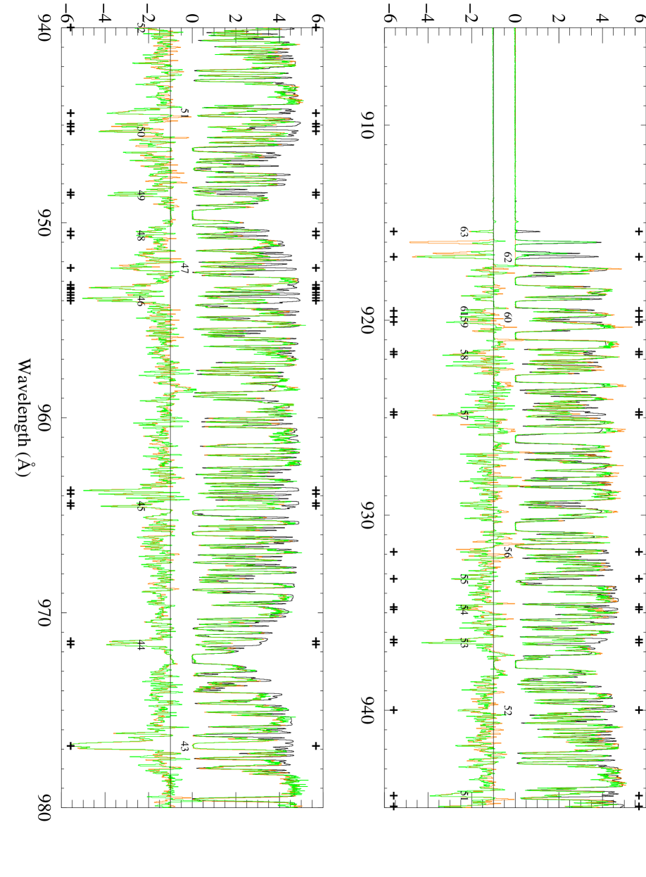
Figure 2a.— Hydrogen absorbed continuum model 905 – 980 Å. Identified line blends are numbered and marked with upper and lower + and tabulated in Table  2. Upper portion of each panel is an overplot of the s12 (orange) and s21 (green) FUSE spectra, and the model (black). Lower portion of each panel shows the data after subtraction of the model, offset by 10^-12 ergs cm^-2 s^-1 Å^-1.

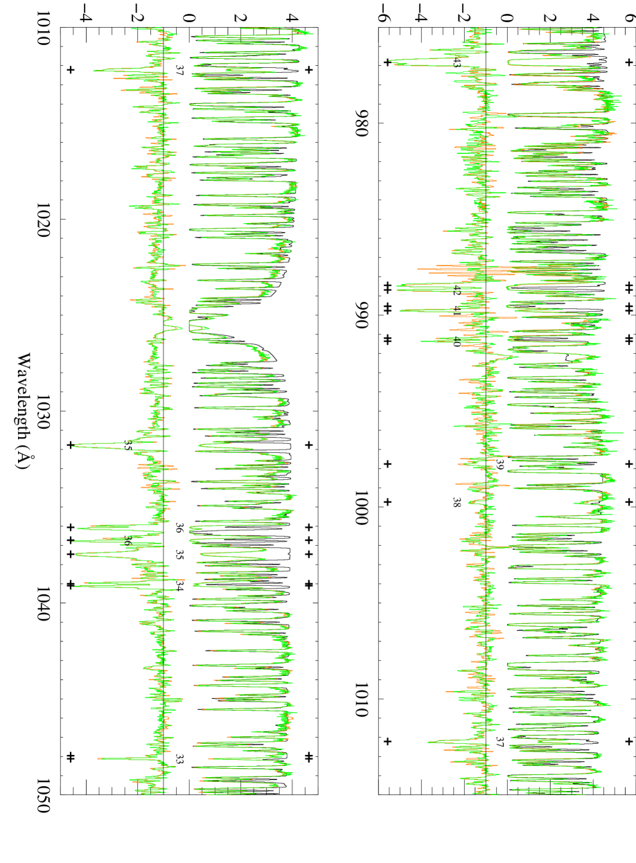
Figure 2b.— Hydrogen absorbed continuum model 975 – 1050 Å. See Figure 2a for a description of the colors and symbols.

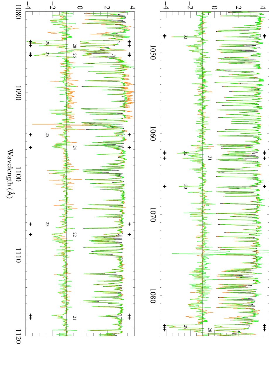
Figure 2c.— Hydrogen absorbed continuum model 1045 – 1120 Å. See Figure 2a for a description of the colors and symbols.

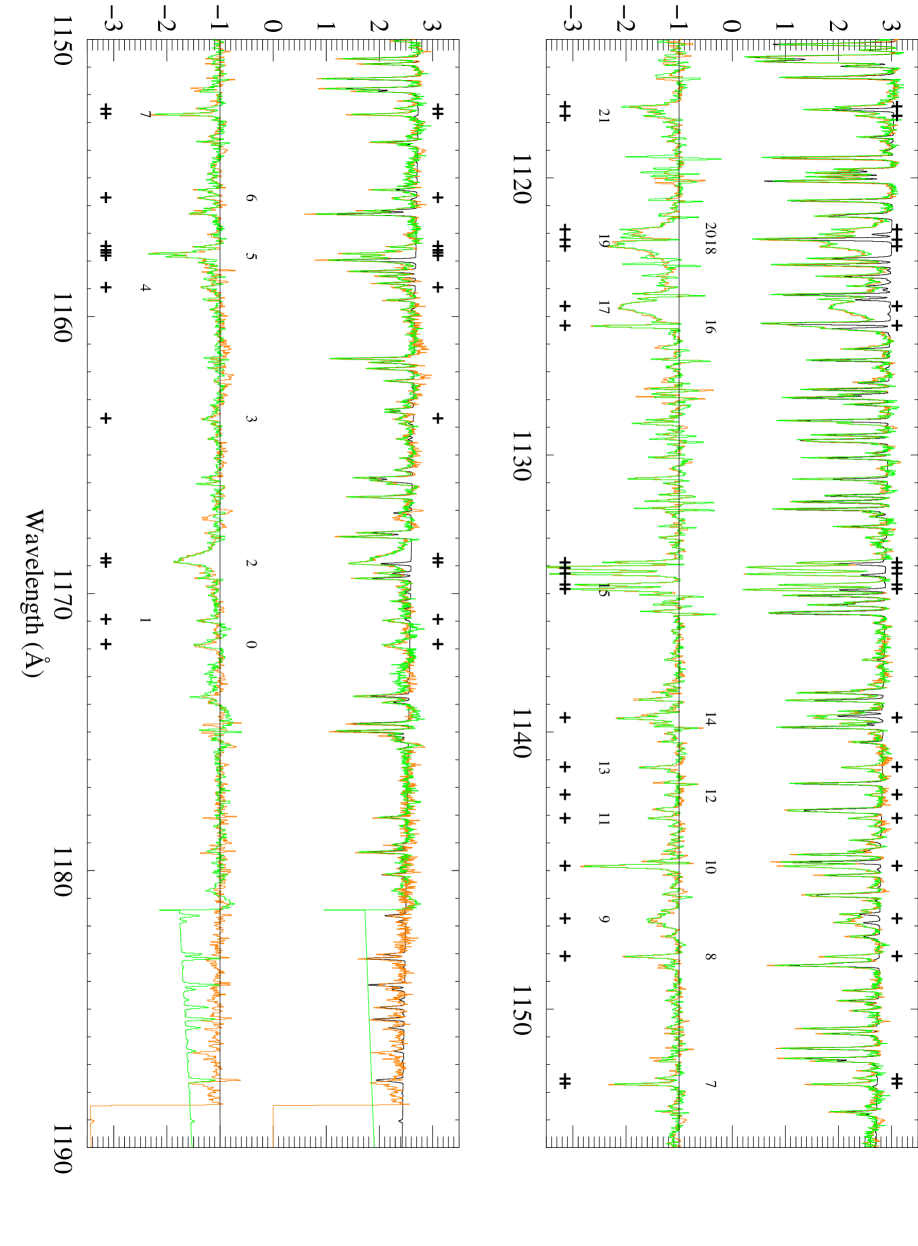
Figure 2d.— Hydrogen absorbed continuum model 1115 – 1190 Å. See Figure 2a for a description of the colors and symbols.

3. Model of Continuum Absorption by Hydrogen and Line Identifications

A model of the CS SED, including the atomic and molecular hydrogen absorptions has been developed by McCandliss et al. (2007) to aid identification of photospheric, nebular or non-nebular velocity components in the FUSE and STIS metal line profiles. We used synthetic stellar flux interpolated from the grid of Rauch (2003) with $\log{g}$ = 6.5, T = 120,000 K, and ratio of H/He = 10/3 by mass. This model includes no metals and is consistent with, although slightly hotter than, the quantitative spectroscopy of Napiwotzki (1999). The adopted temperature and gravity has slightly less pressure broadening and is a better match to the observed Lyman lines towards the series limit. We also adopt a stellar mass of 0.56 $M_{\sun}$ as suggested by post asymptotic giant branch evolutionary tracks. Use of this mass along with the above gravity required a distance of 466 pc to match the absolute flux, which is at the upper limit given by Benedict et al. (2003). Beyond our immediate need to match the absolute flux for the given gravity and mass there is no particular reason to prefer this distance over that derived by Benedict et al. Questions regarding the acceptable uncertainty in distance, absolute flux and derived stellar parameters are best left for a stellar model specifically tailored to include the effects of metals, gravity and evolutionary state. The data supplied here is intended to enable such an effort.

Table 2Stellar, Nebular and Non-Nebular Line ID’s

Feature	$\lambda_{obs}$	Atomic ID, $\lambda_{rest}$	Component
	Å	Å
0	1171.85	O VI 1172.439?	Ph?
1	1170.95	O VI 1171.561?	Ph?
2	1168.90	C IV 1168.993	Ph
…	1168.75	C IV 1168.849	Ph
3	1163.70	?	?
4	1158.97	P II** 1159.087	NN
5	1157.83	C I UV15.01+16	Nb,NN
…	1157.72	C I UV15.01+16	Nb,NN
…	1157.63	C I UV15.01+16	Nb,NN
…	1157.48	C I UV15.01+16	Nb,NN
6	1155.73	C I UV19	Nb,NN
7	1152.71	P II 1152.818	NN
…	1152.53	P II 1152.818	Nb
8	1148.11	?	?
9	1146.75	O VI 1147.072 + 1146.791	Ph
10	1144.85	Fe II 1144.938	NN
11	1143.13	Fe II 1143.226	NN
12	1142.28	Fe II 1142.366	NN
13	1141.28	?	?
14	1139.50	C I 1139.793 (UV22)	Nb
15	1134.86	N I 1134.980	NN
…	1134.70	N I 1134.980	Nb
…	1134.30	N I 1134.415	NN
…	1134.10	N I 1134.415 + 1134.1653	Nb+NN
…	1133.90	N I 1134.165	Nb
16	1125.35	Fe II 1125.448	NN
17	1124.65	O VI 1124.809 +1124.716	Ph
18	1122.49	O VI 1122.618 + C I UV27	Ph,Nb
19	1122.25	O VI 1122.348	Ph,Nb
20	1121.88	Fe II 1121.975	NN
21	1117.78	C I UV29	Nb,NN
…	1117.44	C I UV29	Nb,NN
22	1107.48	C IV 1107.593	Ph
23	1106.21	C I 1106.316	NN
24	1096.78	Fe II 1096.877	NN
25	1095.20	?	?
26	1085.42	N II** 1085.710	Nb
27	1085.25	N II** 1085.551 + 1085.533	Nb
28	1084.23	N II* 1084.584 + 1084.566	Nb
29	1083.90	N II 1083.994	NN
…	1083.70	N II 1083.994	Nb
30	1066.57	Ar I 1066.660	NN
31	1063.09	Fe II 1063.176	NN
32	1062.47	S IV 1062.664	Ph,Nb
…	1062.35	S IV 1062.664	Nb
33	1048.14	Ar I 1048.220	NN
…	1047.98	Ar I 1048.220	Nb
34	1039.12	O I 1039.230	NN
…	1039.02	O I 1039.230	Nb
35	1037.48	O VI 1037.617	Ph
36	1036.75	C II* 1037.018	Nb
36	1036.08	C II 1036.337	Nb
35	1031.79	O VI 1031.926	Ph
37	1012.24	S III 1012.495	Nb
38	999.76	?	?
39	997.78	P III 998.000	Nb
40	991.38	N III 991.577 + 991.511	Nb
…	991.22	N III 991.577 + 991.511	Nb?
41	989.79	Si II 989.873	NN
…	989.56	N III 989.799	Nb
42	988.71	O I 988.773	NN
…	988.47	O I 988.773 + 988.6549	Nb,NN
43	976.85	C III 977.020	Ph,Nb,NN
44	971.65	O I 977.738	NN
…	971.48	O I 977.738	Nb
45	964.54	N I 964.626	NN
…	964.40	N I 964.626	Nb
…	963.93	N I 963.990	NN
…	963.74	N I 963.990 +P II 963.801	Nb
46	954.02	N I 954.104	NN
…	953.88	N I 954.104 + 953.970	Nb,NN
…	953.73	N I 953.970	Nb
…	953.60	N I 953.655	NN
…	953.43	N I 953.655	Nb
…	953.35	N I 953.415	NN
…	953.21	N I 953.415	Nb
47	952.34	N I 952.415	NN
48	950.67	O I 950.885	Nb
…	950.47	P IV 950.657	Nb+(Ph?)
49	948.60	O I 948.686	NN
…	948.47	O I 948.686	Nb
50	945.33	C I 945.579	Nb
…	945.09	C I 945.338	Nb
…	944.95	C I 945.191	Nb
51	944.40	S VI 944.523	Nb+Ph
52	940.01	?	?
53	936.55	O I 936.623	NN
…	936.40	O I 936.623	Nb
54	934.85	?	?
…	934.73	?	?
55	933.28	S VI 933.378?	?
56	931.90	Ar II* 932.054	Nb
57	924.87	O I 924.950	NN
…	924.73	O I 924.950	Nb
58	921.77	O I 921.857	NN
…	921.64	O I 921.857	Nb
59	920.11	?	?
60	919.85	?	?
61	919.54	Ar II 919.781?,O I 919.658?	?
62	916.77	O I 916.960+916.815	Nb,NN
63	915.47	N II 915.61	Nb,NN

The model atomic and molecular absorption spectrum was created by adding to a master optical depth template, covering 900 – 1400 Å, all the contributions from the atomic and molecular hydrogen lines for all the velocity components. There are two distinct components with heliocentric velocities of –75 and –28 $\pm$ 2 km s^-1 for molecular hydrogen. The first is associated with the nebular expansion and the second is associated with non-nebular ISM. For the atomic Lyman series we used transitions up to $n$ = 49, with the velocity offsets, column densities and doppler parameters listed in McCandliss et al. (2007). For hot molecular hydrogen we used the H₂ools rovibrational templates of McCandliss (2003) with b = 7 km s^-1, offset by –75 km s^-1and scaled to the column densities listed in McCandliss et al. (2007). We extended the calculation up to $J\arcsec$= 15 and $v\arcsec$= 3 by assuming the upper level ro-vibration populations were thermal with a temperature of 2040 K as given by the best fit single temperature model. We also used the H₂ools templates to model the cold molecular component at –28 km s^-1 with a pure thermal distribution of 200 K. The transmission function, defined as the negative exponential of the master optical depth template, is multiplied to the stellar continuum model, which has been blueshifted to the systemic radial velocity of the nebula, –42 km s^-1, to produce the model of continuum absorption by hydrogen. This model is also made available on the H₂ools website.

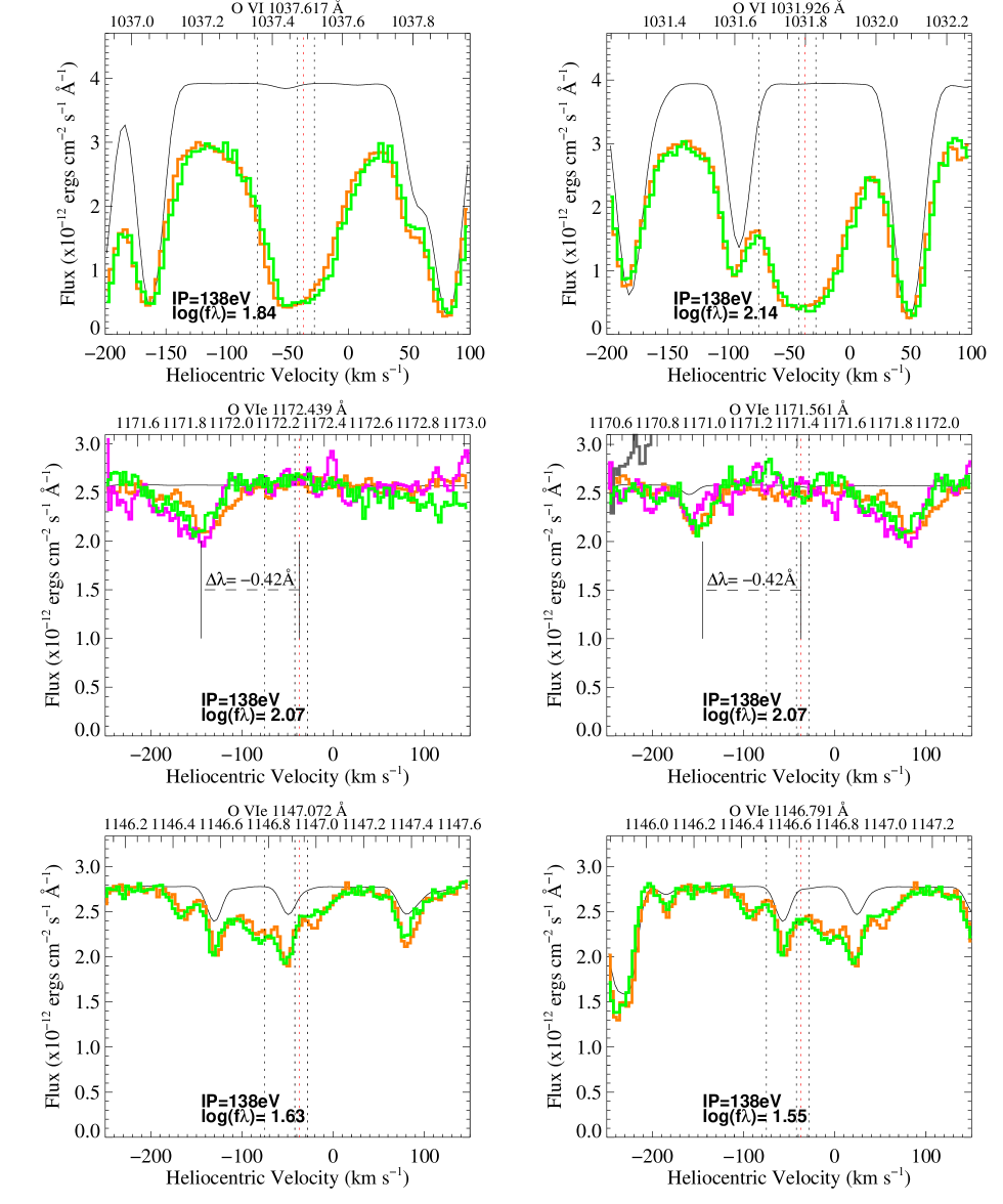
Figure 3.— Stellar photospheric O VI and O VIe lines. FUSE spectra s12 (orange), s21 (green) and the model (black) are plotted along with overlapping STIS orders (purple and grey), if available. Vertical dashed lines mark the transition, $V_{sys}$, $V_{gr}$ and non-nebular velocities at –75, –42, –37 and –28 km s^-1 respectively. O VIe $\lambda\lambda$1172.439, 1171.561 lines were used to assess the offset between the FUSE and STIS spectra. Published rest wavelengths for these lines are discrepant.

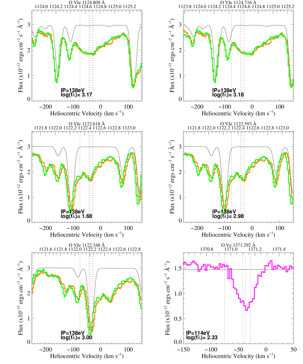
Figure 4.— Stellar photospheric O VIe and O Ve $\lambda$1371.292 lines. Stellar photospheric O VIe and O Ve $\lambda$1371.292 lines. The O Ve $\lambda$1371.292 line was used to established the gravitational redshift of the system. See Figure 3 for a description of the colors.

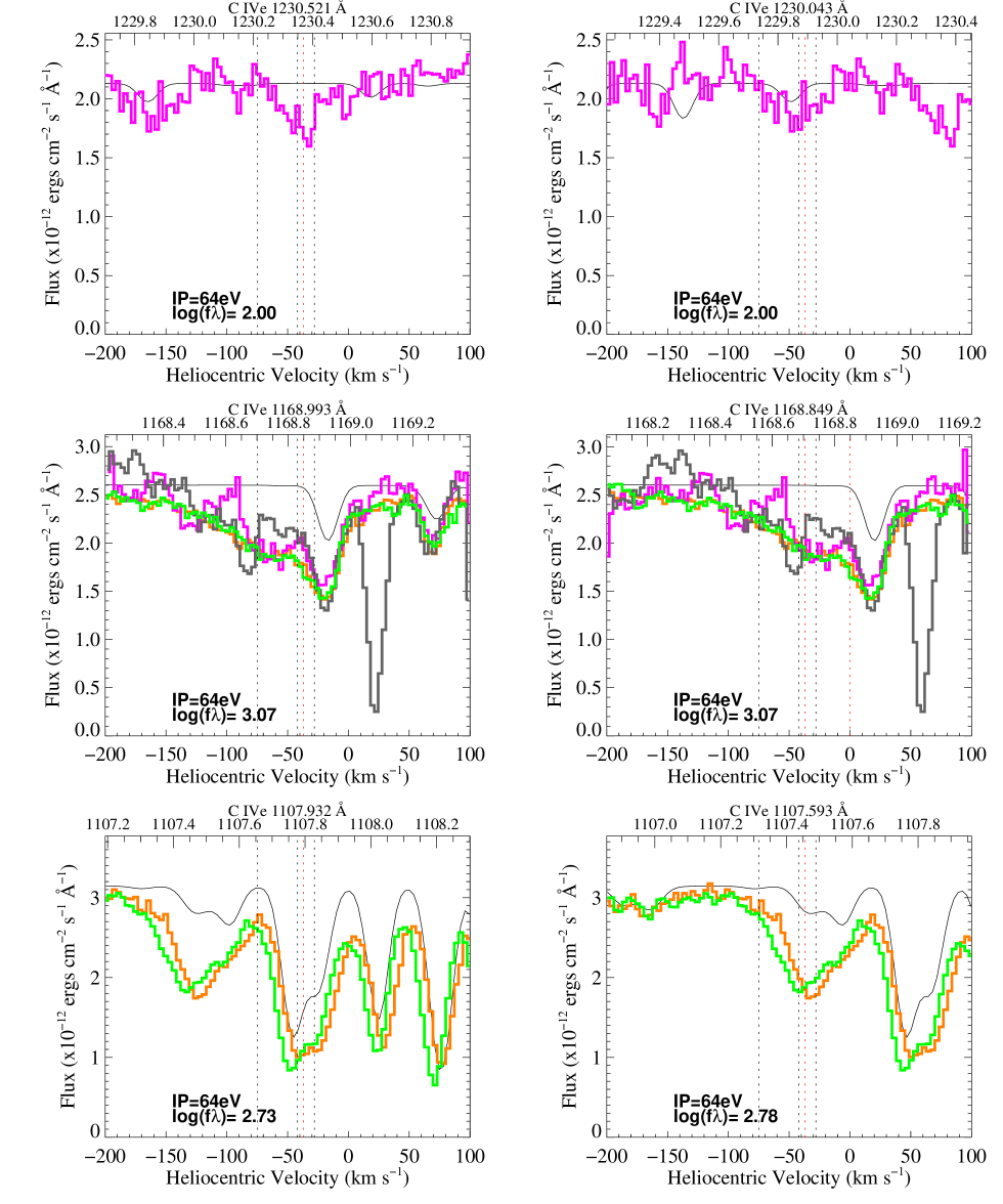
Figure 5.— The photospheric lines of excited C IVe. C IVe $\lambda\lambda$1168.849, 1168.993 were used to reconcile the relative offset between the FUSE and STIS wavelength scales. See Figure 3 for a description of the colors.

Figure 2a shows the resulting continuum absorption model. The top spectral sequence in each panel is an overplot of the s12 (orange) and s21 (green) spectral extractions with the absorbed continuum model (black). The lower sequence in each panel is the residual formed by substracting the model from s12 (orange) and s21 (green). An offset of 10^-12 ergs cm^-2 s^-1 Å^-1 and a two pixel smoothing has been applied to the residuals. The solid horizonal black line marks the zero level for the residuals. The high frequency spikes that go rapidly from positive to negative in the residual are created by local wavelength misalignment of the spectral extractions with respect to the molecular model. The strongest stellar photospheric, nebular and non-nebular absorptions by species other than H₂, H I or photospheric He II are clearly revealed in the residuals. Emission lines of He II $\lambda$1084, $\lambda$992 and $\lambda$958 are also evident. The absorption systems are numbered in the figure in reference to an entry in Table 2 where the line specifications are detailed. The identifications are not exhaustive; small unidentified lines may yet lurk in the noise.

The residual spectrum allows us to assess the success of the absorbed continuum model in reproducing the features in the spectral extractions. Strictly speaking, the subtraction of features should take place in the optical depth space $\tau(\lambda)$ as opposed to the transmission space $\exp(-\tau(\lambda))$. Abundance determinations whether by profile fitting or equivalent width determination must account for the optical depth blending correctly. However, as our purpose here is merely line identification, the simple subtraction process is adequate.

Figure 6.— Absorption as a function of velocity for C IV $\lambda\lambda$1548.204, 1550.781, and N V $\lambda\lambda$1238.821, 1242.804, showing signs of nebular absorption blueward of –37 km s^-1 and photospheric absorption redward. See Figure 3 for a description of the colors.

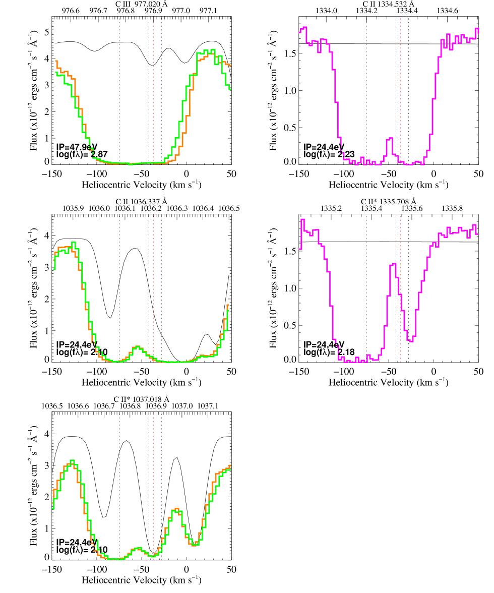
Figure 7.— Absorption as a function of velocity for the C III and C II lines. Like the C IV lines, these lines are heavily saturated throughout the nebular flow region blueward of –42 km s^-1. See Figure 3 for a description of the colors.

Figure 8.— Absorption as a function of velocity for the N III $\lambda\lambda$989.799 – 991.577 multiplet. The N III is blended with molecular hydrogen. The N III* lines are also blended with each other. See Figure 3 for a description of the colors.

Figure 9.— Absorption as a function of velocity for the N II $\lambda\lambda$1083.994 – 1085.710 multiplet. The N II* and N II** lines are blended with each other and molecular hydrogen. The N II line is relatively clean. See Figure 3 for a description of the colors.

Figure 10a.— Absorption as a function of velocity for the N I lines show unsaturated absorption at –75 km s^-1. See Figure 3 for a description of the colors.

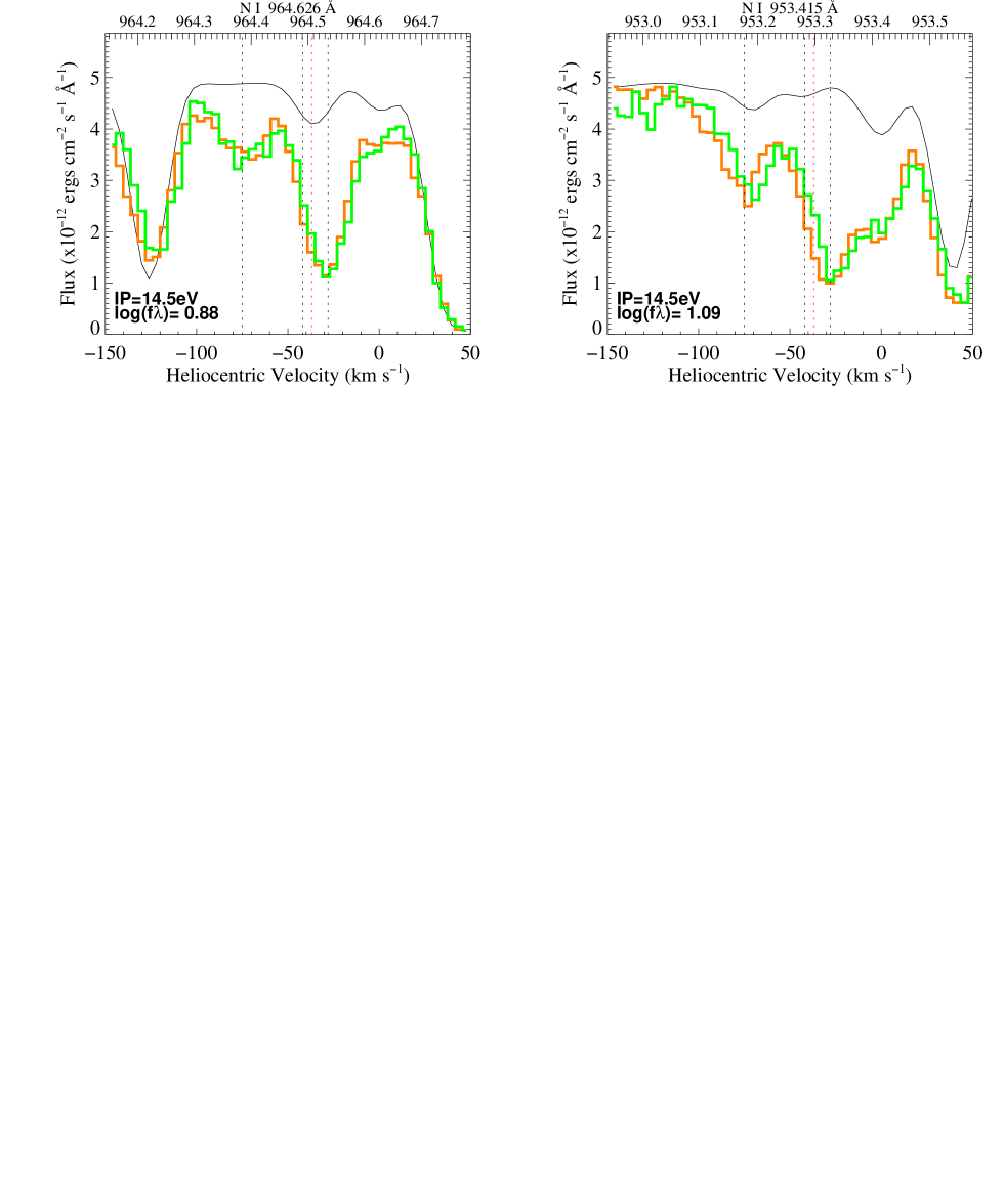
Figure 10b.— More N I lines. See Figure 3 for a description of the colors.

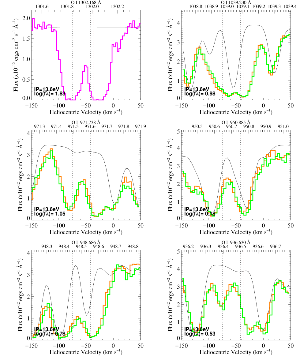
Figure 11.— Absorption as a function of velocity for the O I ground state lines. See Figure 3 for a description of the colors.

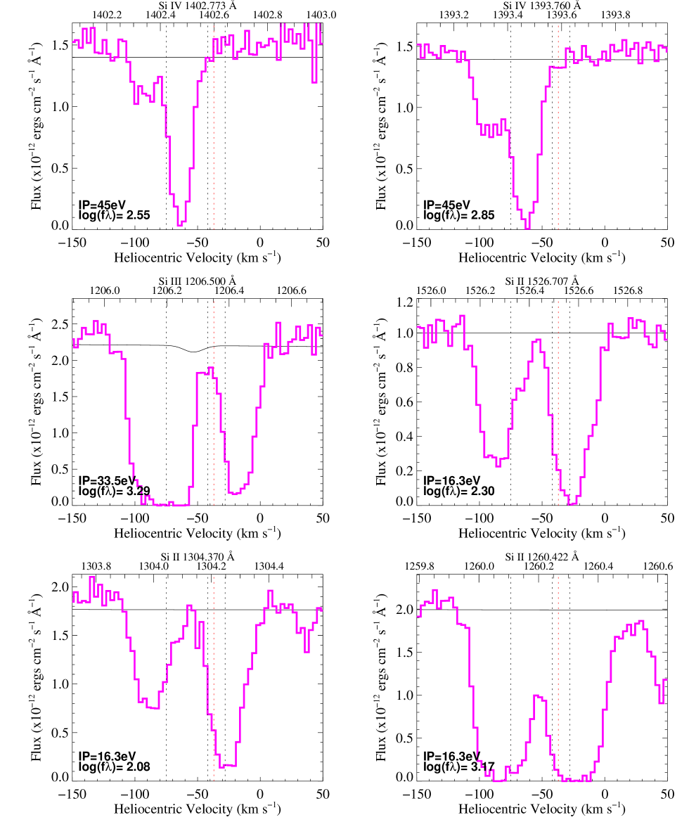
Figure 12a.— Comparision of the Si IV, Si III and Si II. Si II dominates Si IV in the zone between –75 and –110 km s^-1 while Si IV dominates the lower ionization species near –60 km s^-1. See Figure 3 for a description of the colors.

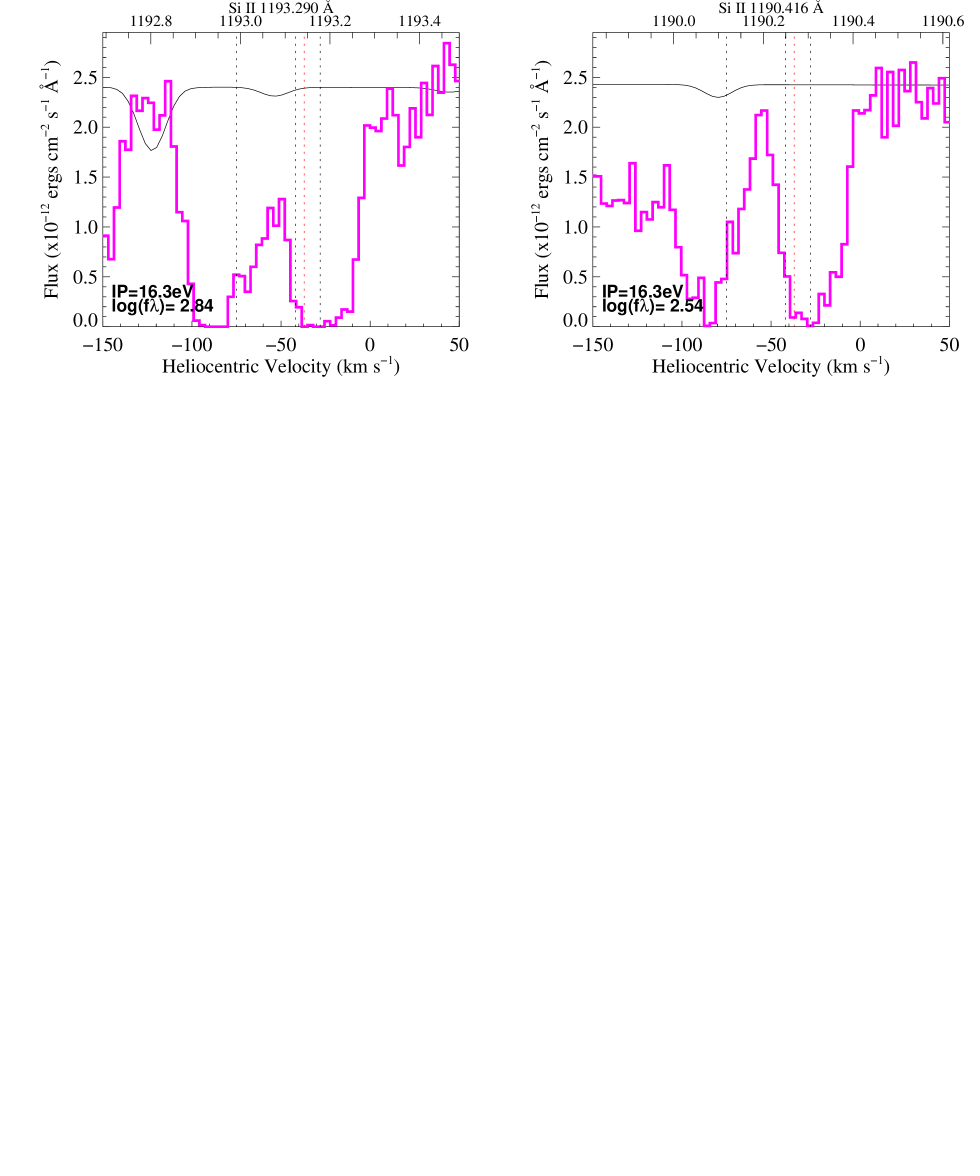
Figure 12b.— More Si II lines. See Figure 3 for a description of the colors.

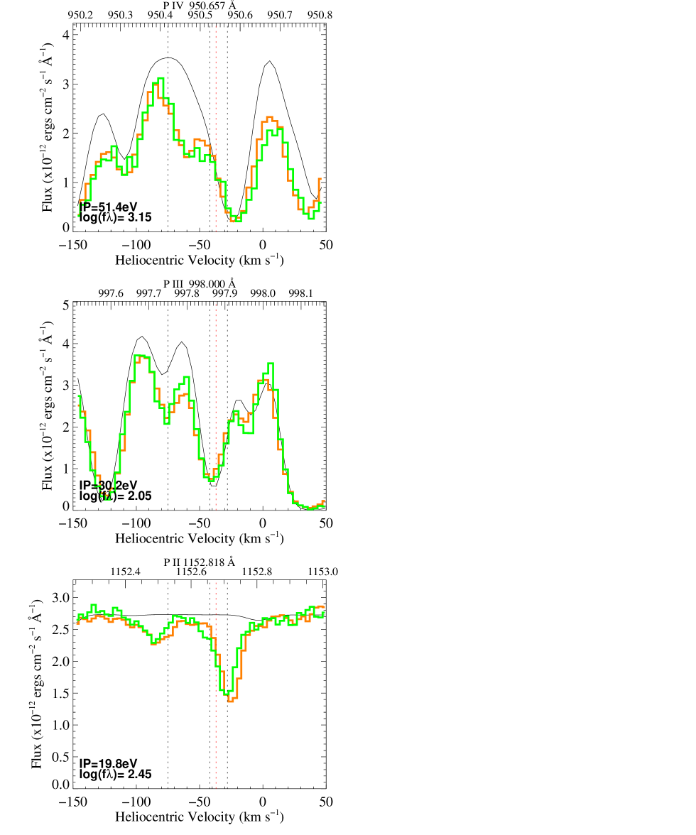
Figure 13.— P IV $\lambda$950.657, P III $\lambda$998.000, and P II $\lambda$1152.818 lines are weak. Although the P IV and P III are surrounded by molecular hydrogen they show behavior similar to Si. See Figure 3 for a description of the colors.

Figure 14.— S IV – S II lines show behavior similar to Si. See Figure 3 for a description of the colors.

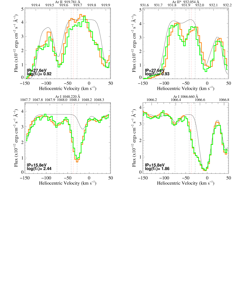
Figure 15.— Ar II lines appear at a velocity of $\approx$ –55 km s^-1, while the Ar I appear at $\approx$ –75 km s^-1. See Figure 3 for a description of the colors.

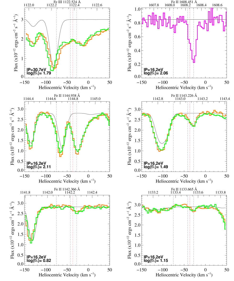
Figure 16.— The detection of Fe III cannot be claimed. Fe II is underabundant relative to S II. See Figure 3 for a description of the colors.

4. STIS and FUSE Absorption Profiles as a Function of Velocity

We separate the display of individual absorption profiles in Figures 3 – 15 into four categories, stellar, nebular plus stellar, nebular CNO and nebular metals. The wider stellar lines we plot over a velocity bandpass of –250 to +150 km s^-1or –200 to +100 km s^-1. Otherwise we use a bandpass of –150 to +50 km s^-1. We omit the broad H I and He II photospheric features. The black dashed vertical lines mark the location of the hot molecular hydrogen component at –75 km s^-1  the systemic velocity at –42 km s^-1, and the cold molecular hydrogen component at –30 km s^-1. The red dashed vertical lines mark the gravitational redshift of the systemic velocity.

The s12 and s21 spectra are shown in orange and green respectively. The continuum model, including the hydrogen lines, is plotted as a thin black line. Regions where the agreement is poor between the wavelength scales for the s12, s21, and model spectra become readily apparent as do regions where the continuum flux is too high, especially near the O VI lines. For lines in the STIS region the spectra are plotted in green.

4.1. Stellar Photospheric Features and the Absolute Wavelength Scale

Comparison of the FUSE and STIS wavelength scales revealed a systematic offset. The reconciliation of this offset is essential for investigating the kinematics of the nebular outflow, where we seek to determine the velocity of the various molecular and atomic features with respect to the systemic velocity of the nebula. In principle, lines that arise from the photosphere should match the systemic velocity of the system less the gravitational redshift offset. In practice this has been difficult to realize except for the narrowest of photospheric features.

We have examined the overlap of the spectra in the common wavelength regions below 1190 Å, where high excitation photospheric C IV and O VI lines are located. We have also checked the registration of the excited molecular hydrogen lines that appear in the STIS bandpass above 1190 Å with the continuum plus hydrogen model. The disagreements revealed from these examinations have been reconciled as described below.

An absolute reference to the heliocentric velocity was established by close examination of the O V $\lambda$1371.296 feature. This narrow line is a transition between two highly excited states in O V and is expected to be an excellent indicator of the photospheric restframe (Pierre Chayer private communication). For a compact object of the mass and radius found by Napiwotzki (1999) we expect the photospheric lines to experience a gravitation redshift, $V_{gr}=c((1-\frac{2GM_{*}}{R_{*}c^{2}})^{-\text@frac{1}{2}}-1$) = 5.1 km s^-1. Applying a shift of –13 km s^-1 to the STIS spectrum placed the centroid of the O V $\lambda$1371.296 at –37 km s^-1, as expected for a $V_{sys}$ of -42 km s^-1 (Wilson, 1953).

In the original analysis of the FUSE M27 spectra by McCandliss (2001) the hot nebular molecular hydrogen component was defined to be at –69 km s^-1. Examining the overlap of common wavelength features in the FUSE and STIS spectra after defining the O V $\lambda$1371.296 to be at –37 km s^-1, we found it necessary to shift the FUSE spectra blueward by –6 km s^-1, such that the hot nebular molecular hydrogen is now at –75 km s^-1. The most useful overlap lines for assessing the alignment were the doublet blend of C IV $\lambda\lambda$1168.849, 1168.993 and the the narrow O VI $\lambda\lambda$1171.56, 1172.44. We note that the wavelengths of the O VI doublet given in the NIST online tables appear to be in error by $\approx$ –0.42 Å. Jahn et al. (2006) have produced an new empirical set of O VI wavelengths, which agree to within 0.04 Å of those found here. We also examined the FUSE N I multiplets at $\lambda\lambda$1134 – 1135 and the STIS N I multiplets at $\lambda\lambda$1200 – 1201 to confirm the wavelength reconciliation.

O VI and O Ve

In Figure 3 and  4 we show the O VI and O V profiles we have identified as being photospheric in origin. Those lines that arise from absorption out of energy levels well above the ground state are designated as either O VIe or O Ve. The O VI $\lambda$1037.62 resonance line shows some very slight signs of blue shifted nebular absorption.

C IVe

In Figure 5 we show the excited C IVe lines. None of these lines is saturated. Overlapping STIS spectra if available are plotted in purple (and grey if two orders are available). These spectra are comparatively noisy, but the alignment with the FUSE spectra agrees as well as the alignment between the s12 and s21 spectra. We note that the error in the systemic velocity is of order the STIS resoution element and is three times the FUSE resolution element. We consider the agreement of line profiles from spectra acquired with two different instruments to be excellent. The STIS order, shown in grey, of the C IVe $\lambda\lambda$1168.849, 1168.993 doublet has a spurious absorption feature that does not appear in the order shown in purple nor in the FUSE spectra and can be ignored.

4.2. Photospheric + Nebular Features

C IV and N V

The high ionization resonance doublets C IV $\lambda\lambda$1548.204, 1550.781, and N V $\lambda\lambda$1238.821, 1242.804 show signs of nebular absorption to the blue of –37 km s^-1 and photospheric absorption to the red as can be seen in Figure 6. The nebular absorption component in the N V lines is strong only between –42 and –75 km s^-1 and is just barely saturated at $\approx$ -60 km s^-1. In contrast, the nebular absorption component in the C IV lines spans –42 to –115 km s^-1 and is completely saturated from –50 to –95 km s^-1.

4.3. Nebular CNO

In general, these lines show absorption from the nebula to the blue, and varying strengths of the intervening (non-nebular) ISM absorption components to the red of the systemic velocity. The nebular features that show absorption only in the nebular expansion (i.e. at velocities blueward of the systemic velocity) are from intermediate or low ionization species. The non-nebular velocity features are most prominent in the lowest ionization and neutral species along the line-of-sight.

C III and C II

We show lines of C III and C II in Figure 7. Like the C IV lines, these lines are heavily saturated throughout the nebular flow region blueward of –42 km s^-1. The saturation makes it difficult to tell, which if any, ion is dominant in the different nebular velocity regimes.

N III, N II and N I

The N III lines in Figure 8 are strongly blended with overlapping molecular hydrogen. The blended profile indicates the absorption is saturated between –60 and –100 km s^-1. The N II* and N II** lines in Figure 9 are similarily messy. However, N II $\lambda$1083.994 is relatively clean. It shows absorption throughout the flow, being less saturated at low velocities and becoming completely saturated at –75 km s^-1. This line also shows stonger nebular absorption than non-nebular absorption emphasizing its dominance over N I, which shows the opposite behavior. The N I multiplets at $\lambda\lambda$1134.165 – 1134.980 and $\lambda\lambda$1199.550 – 1200.710, in Figure 10a, simply show unsaturated absorption centered at –75 km s^-1.

O I

The O I lines in Figure 11 show a range of saturated to unsaturated profiles centered at –75 km s^-1. It may be possible to determine the column density of this species fairly accurately with a curve of growth, after properly accounting for the continuum placement and molecular hydrogen optical depth subtraction.

4.3.1 Nebular Metals

The transition zone between high ionization and low ionization occurs at the velocity of –75 km s^-1, where H I, C I, N I, O I and molecular hydrogen show up most strongly in the nebula.

Si IV, Si III and Si II

The high ionization low velocity, low ionization high velocity dichotomy is most clearly seen in the Si IV $\lambda$1393.760 and Si II $\lambda$1193.290 lines as shown in Figure 12a. Since these lines have nearly equal $\log(f\lambda)$ they are reliable indicators of the relative ionization as a function of velocity. Si II is stronger than Si IV in the zone between –75 and –110 km s^-1, while Si IV is stronger than Si II in the zone between –42 and –75 km s^-1. The Si III $\lambda$1206.500 line is saturated throughout most of the flow. It is a very strong line with a $\log(f\lambda)$ = 3.29, which makes it difficult to determine if this species is the dominant ion throughout the flow.

P IV, P III and P II

We detect weak P IV $\lambda$950.657, P III $\lambda$998.000, and P II $\lambda$1152.818 at progressively high velocities of $\approx$ –65, –70, –80 km s^-1 respectively as shown in Figure 13. The P V $\lambda$1117.977 line (not shown) of the P V doublet is very weak, while $\lambda$1128.008 is blended with H₂.

S IV, S III and S II

The S IV – S II ions show similar behavior to Si and P in Figure 14. The S III $\lambda$1190.203 line appears to have a feature near –42 km s^-1. However, this is just the nebular component of the nearby Si II $\lambda$1190.416 line. The nebular portion of this feature is clean and agrees well with the shape of the S III $\lambda$1012.495 profile, with the absorption stongest near –70 km s^-1and weakening slowly to the blue and relatively quickly to the red.

Ar II and Ar I

Figure 15 shows Ar II $\lambda$919.781, Ar II* 932.054, and Ar I 1048.220 are detected, with Ar II appearing at $\approx$ –55 km s^-1 and Ar I appearing at $\approx$ –75 km s^-1. Ar I 1066.660 is blended with an overlapping H₂ line. Ar II 919.781 is blended with a nearby molecular hydrogen line but the nebular Ar II* $\lambda$932.054 is clearly visible without model subtraction. The thermal production of Ar II* requires a temperature $\sim$ 10,000 K, and is a confirmation that the gas at low velocities is much hotter than that indicated by the molecular hydrogen. The absorption of the Ar II lines is stronger than the Ar I lines even though they have transition strengths a factor of 10 lower. This suggests the Ar II is the dominant over Ar Iin the nebula.

Fe III and Fe II

Fe III $\lambda$1122.524 may be blended with a molecular hydrogen line aon the blue side of the photospheric O VIe $\lambda\lambda$1122.593 – 1122.618 doublet as shown in Figure 16. However, without a good idea of what the photospheric line shape is in this region, we cannot claim a detection. The strongest transitions of Fe II $\lambda$1608.451 and $\lambda$1144.938 appear weakly at –75 km s^-1. These lines have transition strengths ($\log{(f\lambda)}$ = 2.06, 2.11) that are nearly identical to that of Si II $\lambda$1304.370 ($\log{(f\lambda)}$ = 2.08), yet the Si II feature is much stronger. The ionization potential of Si II (16.3 eV) is also nearly identical to that of Fe II (16.2 eV) and they also have similar condensation temperatures (Morton, 2003). We conclude that Fe II relative to Si II is underabundant in the nebula.

Arguing in a similar vein, we see that the transition at Fe II $\lambda$1133.665 is not detected in the nebula at all. It has nearly the same transition strength ($\log{(f\lambda)}$ = 1.15) as the S II $\lambda$1253.811 line ($\log{(f\lambda)}$ = 1.14), which is weak but easily seen. We conclude that Fe II relative to S II is also underabundant. The solar abundance of Si and Fe are nearly identical (7.56, 7.50 respectively) and are slightly higher than S (7.2). It is not unusual to have the Si abundance greater than the Fe in the typical ISM because it is depleted onto dust (Savage & Sembach, 1996). However, here we have no Fe in the gas phase and appearently very little dust in the diffuse nebular medium. This is a puzzle.

5. Suggestions for Future Investigations

M27 is a excellent laboratory for testing theories regarding the abundance kinematics in PNe because the stellar temperature, mass, gravity, and the nebular mass, distance, abundances, extinction and excitation states, are well quantified. The reduced spectra provided by this study and the associated atomic and molecular hydrogen model for the nebular and non-nebular absorptions, should enable a photospheric analysis of the metal abundances, similar to the effort undertaken by Jahn et al. (2006) for PG 1159 - 035. Establishing a reliable stellar continuum is the first step towards determining accurate nebular absorption line abundances for comparision with those derived from the emission line analyses of Barker (1984) and Hawley & Miller (1978).

The finding in Paper I, of little extinction by dust in the nebula raises a number of interesting questions concerning the depletion of metals in the diffuse and clumpy media, which go beyond the scope of this investigation. A major limitation to this effort is the requirement for a good stellar model that can reliably reproduce the observed photospheric features and continuum, especially in the vicinity of the blend of nebular Fe III $\lambda$1122.52 with photospheric O VI $\lambda$1122.62. If such a stellar model can be produced, the total S, Si, P and Fe abundances should be derivable by profile modeling after accounting for the atomic and molecular hydrogen absorption provided here. The question of whether the abundances of these metals change across the neutral transition zone could provide information on whether photo-evaporation of the globules is an important process for the enrichment of metals in the high velocity zone. A model of the nebular ionization as a function of velocity would be useful for this purpose. Such a model might be produced by melding the detailed time dependent approach to the calculations of the atomic and molecular emissions followed by Natta & Hollenbach (1998), with the radiative hydrodynamical rigor of Villaver et al. (2002). The problem may also be approached by using the Sobolev plus exact integration (SEI) method of Lamers et al. (1987), from which a empirical parameterization of the wind velocity ‘law” could be obtained.

;

References

- Bachiller et al. (2000) Bachiller, R., Cox, P., Josselin, E., Huggins, P. J., Forveille, T., Miville-Deschênes, M. A., & Boulanger, F. 2000, in ESA SP-456: ISO Beyond the Peaks: The 2nd ISO Workshop on Analytical Spectroscopy, 171
- Barker (1984) Barker, T. 1984, ApJ, 284, 589
- Benedict et al. (2003) Benedict, G. F., et al. 2003, AJ, 126, 2549
- Hawley & Miller (1978) Hawley, S. A., & Miller, J. S. 1978, PASP, 90, 39
- Jahn et al. (2006) Jahn, D., Rauch, T., E., R., Werner, K., Kruk, J. W., & Herwig, F. 2006, Accepted å
- Kwok et al. (1978) Kwok, S., Purton, C. R., & Fitzgerald, P. M. 1978, ApJ, 219, L125
- Lamers et al. (1987) Lamers, H. J. G. L. M., Cerruti-Sola, M., & Perinotto, M. 1987, ApJ, 314, 726
- Lupu et al. (2006) Lupu, R., France, K., & McCandliss, S. R. 2006, ApJ
- McCandliss (2001) McCandliss, S. R. 2001, in ASP Conf. Ser. 247: Spectroscopic Challenges of Photoionized Plasmas, 523
- McCandliss (2003) McCandliss, S. R. 2003, PASP, 115, 651
- McCandliss et al. (2007) McCandliss, S. R., France, K., Lupu, R., Burgh, B. B., Sembach, K., Kruk, J., Andersson, B.-G., & D., F. P. 2007, to be submitted to ApJ
- Meaburn & Lopez (1993) Meaburn, J., & Lopez, J. A. 1993, MNRAS, 263, 890
- Meaburn (2005) Meaburn, J. 2005, ArXiv Astrophysics e-prints, arXiv:astro-ph/0512099
- Meaburn et al. (2005a) Meaburn, J., Boumis, P., Christopoulou, P. E., Goudis, C. D., Bryce, M., & López, J. A. 2005, Revista Mexicana de Astronomia y Astrofisica, 41, 109
- Meaburn et al. (2005b) Meaburn, J., Boumis, P., López, J. A., Harman, D. J., Bryce, M., Redman, M. P., & Mavromatakis, F. 2005, MNRAS, 360, 963
- Moos et al. (2000) Moos, H. W., et al. 2000, ApJ, 538, L1
- Morton (2003) Morton, D. C. 2003, ApJS, 149, 205
- Napiwotzki (1999) Napiwotzki, R. 1999, A&A, 350, 101
- Natta & Hollenbach (1998) Natta, A., & Hollenbach, D. 1998, A&A, 337, 517
- O’Dell et al. (2002) O’Dell, C. R., Balick, B., Hajian, A. R., Henney, W. J., & Burkert, A. 2002, AJ, 123, 3329
- Quijano (2003) Quijano, e. a., J. K. 2003, STIS Instrument Handbook, Version 7.0 (STIS Instrument Handbook, by Spectrographs Group, (Baltimore: STScI))
- Rauch (2003) Rauch, T. 2003, A&A, 403, 709
- Sahnow et al. (2000) Sahnow, D. J., et al. 2000, ApJ, 538, L7
- Savage & Sembach (1996) Savage, B. D., & Sembach, K. R. 1996, ARA&A, 34, 279
- Villaver et al. (2002) Villaver, E., Manchado, A., & García-Segura, G. 2002, ApJ, 581, 1204
- Wilson (1953) Wilson, R. E. 1953, in Carnegie Institute Washington D.C. Publication, 0
;