The XMM-Newton wide-field survey in the COSMOS field: V. Angular Clustering of the X-ray Point Sources

Abstract

We present the first results of the measurements of angular auto-correlation functions (ACFs) of X-ray point sources detected in the XMM-Newton observations of the $\sim$ 2 deg² COSMOS field (XMM-COSMOS). A significant positive signals have been detected in the 0.5-2 (SFT) band, in the angle range of 0.5-24 arcminutes, while the positive signals were at the $\sim$2 and $\sim 3\sigma$ levels in the 2-4.5 (MED) and 4.5-10 (UHD) keV bands respectively. Correctly taking integral constraints into account is a major limitation in interpreting our results. With power-law fits to the ACFs without the integral constraint term, we find correlation lengths of $\theta_{\rm c}=1\farcs 9\pm 0\farcs 3$, $0\farcs 8^{+0\farcs 5}_{-0\farcs 4}$ and $6\arcsec\pm 2\arcsec$ for the SFT, MED, and UHD bands respectively for $\gamma=1.8$. The inferred comoving correlation lengths, also taking into account the bias by the source merging due to XMM-Newton PSF, are $r_{\rm c}\approx 9.8\pm 0.7$, $5.8^{+1.4}_{-1.7}$ and $12\pm 2$ $h^{-1}$ Mpc at the effective redshifts of $\bar{z}_{\rm eff}\approx$ 1.1, 0.9, and 0.6 for the SFT, MED, and UHD bands respectively. If we include the integral constraint term in the fitting process, assuming that the power-law extends to the scale length of the entire XMM-COSMOS field, the correlation lengths become larger by $\sim 20$%–90%. Comparing the inferred rms fluctuations of the spatial distribution of AGNs $\sigma_{\rm 8,AGN}$ with those of the underlying mass, the bias parameters of the X-ray source clustering at these effective redshifts are in the range $b_{\rm AGN}=1.5-4$.

1 Introduction

Results from recent X-ray surveys have made very significant contributions to understanding formation and evolution of supermassive blackholes (SMBHs) at galaxy centers. In particular, studies of X-ray luminosity function and its evolution have been providing the most reliable current estimates of the accretion history to SMBH. One of the most important findings in recent years is that luminous active galactic nuclei (AGNs) arise earlier in the history of the universe than lower luminosity ones (Ueda et al., 2003; Hasinger et al., 2005; Barger et al., 2005; La Franca et al., 2005). This suggests that more massive SMBHs have been formed earlier in the universe, and reside quiescently at the centers of giant elliptical galaxies in the later epochs, while more numerous, less massive SMBHs have been formed and accreted later in the history of the universe.

Clustering properties of AGNs and their evolution with redshift provide yet additional clues to understanding the accretion processes onto the SMBHs. These give clues to environments of AGN activities. In the framework of the Cold Dark Matter (CDM) structure formation scenario, clustering properties or the bias of AGNs over a sufficiently large scale $b_{\rm AGN}=(\delta\rho/\rho)_{\rm AGN}/(\delta\rho/\rho)_{\rm mass}$ may be related to the typical mass of dark matter halos in which they reside, (Mo & White, 1996; Sheth et al., 2001). At the same time, the mechanisms of triggering the AGN activity, which might be closely related to galaxy interactions and/or merging (Menci et al., 2004; Di Matteo et al., 2005), yield a clustering of AGNs and can therefore be infered from the clustering analysis.

Since strong X-ray emission is a typical feature of an AGN activity, X-ray surveys provide most efficient means of constructing comprehensive complete samples of AGNs without contamination from the light in the stellar population of host galaxies. In particular, surveys in the harder ($E>2$ keV) X-ray band such as available from XMM-Newton are very efficient in finding not only unobscured AGNs, which are relatively easy to select also in the optical bands, but also obscured ones, which are difficult to select with optical selection criteria alone. This is important because most of the accretion ($\sim 80$%; Comastri et al., 1995; Gilli et al., 2001; Ueda et al., 2003) occurs in AGNs obscured by gas (in X-ray bands) and dust (in the optical bands). While one approach in investigating the environment of AGNs is to measure AGN overdensities around known clusters of galaxies (Cappi et al., 2001; D’Elia et al., 2004; Cappelluti et al., 2005), a more common and direct measure can be obtained by calculating auto-correlation functions (ACFs) of well-defined samples of X-ray selected AGNs.

While small number statistics limits the accuracy of the clustering measurements of X-ray selected AGNs, there are a number of reports on the detection of the correlation signals. Samples based on the ROSAT All-Sky survey have mainly constrained the clustering properties of type 1 local AGNs at $z\lesssim 0.3$. The correlation lengths resulting from the angular (Akylas et al., 2000) and 3D (Mullis et al., 2004) analyses of these samples are 6-7 $h^{-1}$ Mpc . Due to the wide redshift distribution, it is more difficult to obtain clustering signal in deeper X-ray surveys before redshifts for a complete set of X-ray sources are obtained. Nevertheless, Basilakos et al. (2004, 2005) measured strong angular correlation signals in their XMM-Newton/2dF survey, which covers a total area of 2 deg² over two fields. They obtained a correlation length of $\sim 7.5\,h^{-1}$ Mpc in physical units for both soft and hard X-ray selected sources, suggesting a clustering evolution which is fixed in the proper coordinate between z$\sim 0$ and $z\gtrsim 1$. At much fainter X-ray fluxes, Gilli et al. (2005) analyzed the projected-distance correlation function $w(r_{\rm p})$ for the X-ray sources with spectroscopic redshifts in the Chandra Deep Fields North (CDF-N) and South (CDF-S). They found significantly different clustering properties in these two fields, suggesting a cosmic variance effect. Recently, Yang et al. (2006) made detailed analysis on their 0.4 deg² Chandra Large Area Synoptic X-ray Survey (CLASXS) supplemented by CDF-N. With spectroscopic redshifts for a good portion of the sources, they explored the clustering properties in different redshift and luminosity bins as well as intrinsic absorption bins. They found the evolution of bias with redshift but they did not find significant dependence in the clustering properties of X-ray selected AGNs based on either luminosity or intrinsic absorption.

One of the main aims of the COSMOS (Scoville et al., 2007) project is to trace the evolution of the large-scale structure of the universe with an unprecedented accuracy and redshift baseline. The XMM-Newton Survey, covering the entire COSMOS field (XMM-COSMOS; Hasinger et al., 2007), is one of the most extensive XMM-Newton Survey programs conducted so far. In the first-year XMM-Newton observations, about 1400 X-ray point sources have been detected and cataloged (Cappelluti et al., 2007) (hereafter C07), which are dominated by AGNs at redshifts $0.7<z<2$ (Brusa et al., 2007; Trump et al., 2007).

In this paper, we report the first results of our investigations on the large scale structure through an angular auto-correlation (ACF) function analysis of the X-ray point sources detected in XMM-COSMOS, as a preview of more detailed studies in the near future. Our future studies include the derivation of the direct three-dimensional correlation function using redshift information already available for a large portion of the X-ray sources and the analysis of the cross-correlation of the X-ray sources with galaxies in the multiwavelength COSMOS catalog.

The outline of the paper is as follows. In Sect. 2, we explain the selection of our samples of X-ray sources to be used in the correlation function analysis, which are subsets of those described in C07. Details of the calculations, including the ACF estimator, the random sample, and power-law fits are presented in Sect. 3. The de-projection to the three-dimensional correlation function is presented in Sect. 4. The results are discussed in Sect. 5. We summarize our conclusions in Sect 6

2 Sample Selection

Our samples consist of the X-ray sources detected in the first-year XMM-Newton observations of the COSMOS field. The source detection, construction of the sensitivity maps, and source counts are described in C06. The X-ray source catalogs in three energy bands, corresponding to energy channels of 0.5-2 (SFT), 2-4.5 (MED) and 4.5-10 (UHD) keV are used.

For the angular ACF studies, we have applied further selection criteria to the C06 sources to minimize the effects of possible systematic errors in the sensitivity maps. The applied criteria for this kind of analysis should be stricter than those adopted for the derivation of the $\log N-\log S$ function, because localized systematic errors may cause spurious clustering of X-ray sources. In order to do this, we have scaled up the original sensitivity map to:

$$CR_{\rm lim,acf}=\max(a\;CR_{\rm lim,C06}-b,\;CR_{\rm lim,min}),$$ (1)

where $CR_{\rm lim,C06}$ is the limiting count rate ( in cts s^-1) in the original C06 sensitivity map and $CR_{\rm lim,acf}$ is the sensitivity map used for the ACF analysis. After a number of trials, the scaling coefficients $(a,b)$ have been set to (1.33,$1\times 10^{-4}$), (1.40, 0.) and (1.44, $4\times 10^{-4}$) for the SFT, MED and UHD bands respectively. We have excluded the area where $CR_{\rm lim,acf}$ exceeds $CR_{\rm lim,max}$ (low exposure areas close to the field borders). Those X-ray sources with $CR$’s below $CR_{\rm lim,acf}$ at the source position have been excluded from the ACF analysis. After these screenings, the numbers of sources for the ACF analysis are 1037, 545, and 151 for the SFT, MED, and UHD bands respectively. While the sensitivity in the soft band is the best among the three bands, some X-ray sources are hard enough that they are detected in only MED and/or UHD bands. These are mainly highly obscured AGNs. Out of the 545 (151) MED (UHD) band sources after the screening process, 59 (13) have not been detected in the SFT band, and only one UHD sources have escaped the detection in the MED band (before the screening process). The numbers of the X-ray sources, values of $CR_{\rm lim,min}$,$CR_{\rm lim,max}$ and the total areas used for the ACF analysis are summarized in Table 1.

3 Angular Correlation Function Calculation

3.1 The ACF calculation

In calculating the binned ACF, we have used the standard estimator by Landy & Szalay (1993):

$$w_{\rm est}(\theta_{i})=(DD-2DR+RR)/RR,$$ (2)

where DD, DR, and RR are the normalized numbers of pairs in the $i$-th angular bin for the data-data, data-random, and random-random samples respectively. Also we use the symbols $D$ and $R$ to represent the data and random samples respectively. Expressing the actual numbers of pairs in these three combinations as $n_{\rm pair,DD}(\theta_{i})$, $n_{\rm pair,DR}(\theta_{i})$ and $n_{\rm pair,RR}(\theta_{i})$, the normalized pairs are expressed by:

$$DD=n_{\rm pair,DD}(\theta_{i})/[N_{\rm D}(N_{\rm D}-1)]$$

$$DR=n_{\rm pair,DR}(\theta_{i})/(N_{\rm D}N_{\rm R})$$

$$RR=n_{\rm pair,RR}(\theta_{i})/[N_{\rm R}(N_{\rm R}-1)]$$ (3)

where $N_{\rm D}$, and $N_{\rm R}$ are the numbers of sources in the data and random samples respectively. The number of objects in the random sample has been set to 20 times of that in the data sample. This makes the variance of the second and third terms of Eq. 2 negligible in the error budget of $w_{\rm est}$.

Our XMM-Newton observations have varying sensitivity over the field. In order to create a random sample, which takes the inhomogeneity of the sensitivity over the field into account, we have taken the following steps.

1. Make a random sample composed of $N_{\rm R}$ objects, where $N_{\rm R}$ is an integer times $N_{\rm D}$.

2. For each random object, assign a count rate from a source from the data sample. The assignments are made in sequence so that the CR distributions of the random and the data sample objects are exactly the same.

3. For each random object, assign a random position in the field. If the sensitivity-map value at this position ($CR_{\rm lim,acf}$ from Eq. 1, in units of counts s^-1) is larger than the assigned CR, find a different position. Repeat this until the position is sensitive enough to detect a point-source with the assigned CR.

As a check on this procedure, we have also calculated ACFs using two other methods of generating random samples. The second method is to assign the count rates to the random sources drawn from a $\log N$ – $\log S$ relation (e.g. Moretti et al., 2003), instead of copying the count rates of the data sample. Then the source is placed at a random position in the field. If the sensitivity limit at this position is higher than the assigned CR, this random source is rejected. Another, but more sophisticated and computationally demanding method is to generate random sources based on the $\log N$ – $\log S$ relation, down to a flux level much lower than the sensitivity limit of our observations. These sources are then fed into a simulator, taking into account XMM-Newton instrumental effects, including position-dependent PSF, exposure maps, and particle background. The entire first-year XMM-COSMOS image has been simulated and the same source detection procedure as that applied to the actual data has been applied on the simulated data. A random sample $R$ is generated from 10 simulated XMM-COSMOS fields. Using the above two methods for random sample generations did not alter the results significantly. In the following analysis, we show the results obtained by the first method.

3.2 Error Estimation and Covariance Matrix

We have estimated the errors using the variance of the calculated ACF by replacing $D$ in Eq. 2 by random samples. A random sample with the same number of objects and the same set of count rates as $D$ has been drawn independently from $R$ in Eq. 2. We denote the random sample as a replacement of $D$ during the error search by $R^{\prime}$ to distinguish from $R$. For each angular bin, a 1 $\sigma$ error has been calculated as a standard deviation from resulting ACFs calculated from $N_{\rm run}=$80 different $R^{\prime}$ samples, which is then multiplied by a scaling factor $[1+w(\theta_{i})]^{1/2}$ (hereafter referred to as “the scaled random errors”). This scaling factor corrects for the difference between the errors in the null-hypothesis case, obtained from $R^{\prime}$s, and those in the presence of the correlation signal. This is in line with the observation that the error in each bin of the ACF calculated using the Landy & Szalay (1993) estimator is approximately a Poisson fluctuation of the number of data-data pairs in the bin, i.e., $\sigma\sim[1+w(\theta)]/\sqrt{n_{\rm pair,DD}}$. The standard deviation of the null-hypothesis ACF, obtained by replacing $D$ by an $R^{\prime}$, is $\sigma_{\rm ran}\sim 1/\sqrt{n_{{\rm pair},R^{\prime}R^{\prime}}}$. The scaling factor can be obtained by using the relation, $n_{\rm pair,DD}\approx[1+w(\theta)]n_{\rm pair,R^{\prime}R^{\prime}}$.

In correlation functions, the errors in different angular bins are not independent from one another and correlations among the errors have to be taken into account when we make function fits. Thus we have also estimated full covariance matrix in order to represent the correlations among errors by

$$M_{{\rm cov},ij} =\sum_{k}(w_{{\rm R},k}(\theta_{i})-\langle w_{\rm R}(\theta_{i})\rangle)$$ (4)

$$\times(w_{{\rm R},k}(\theta_{j})-\langle w_{\rm R}(\theta_{j})\rangle)/N_{\rm run}$$

$$\times(1+w_{\rm est}(\theta_{i}))^{1/2}(1+w_{\rm est}(\theta_{j}))^{1/2}$$

where $w_{{\rm R},k}(\theta_{i})$ is the ACF value for the $k$-th random run ($k$ runs through 1 to $N_{\rm run}=80$), $\langle w_{\rm R}(\theta_{i})\rangle$ is their mean value, evaluated at the center of the $i$-th angular bin $\theta_{i}$ and $w_{\rm est}(\theta_{i})$ is from Eq. 2. The square roots of the diagonal elements of Eq. 4 are the scaled random errors discussed above. The covariance matrix calculated in Eq. 4 is used later in Sect. 3.4. Strictly speaking, Eq. 4 only takes into account the correlations of errors for the random cases, but not the correlation of errors due to clustering. One way of explaining this is that removing/adding one source (by a Poisson chance) affects multiple angular bins and this is represented by non-diagonal elements of Eq. 4. On the other hand, correlation of errors due to large scale structure or the cosmic variance is not represented by this. If we observe another part of the sky, we sample different sets of large scale structures such as filaments and voids. Since the existence or non-existence of one such structure affects multiple angular bins, there should be additional contribution to the non-diagonal elements of the correlations among errors in different angular bins. Eq. 4, based on many random samples, thus includes the former type of the correlation of errors but not the latter. One way to include also the latter effect is to use the Jackknife re-sampling technique, as was done by e.g. Zehavi et al. (2004). However, the Jackknife re-sampling requires to divide the sample into many statistically independent regions, which is not practically possible in our case.

3.3 The binned ACF results

The ACFs have been calculated for the three bands in logarithmically equally spaced bins with $\Delta\log\theta=1/6$. The results are shown in Fig 1, where the upper panels, composed of two layers of logarithmic plots with positive and negative parts ($\log|w(\theta)|>-2.8$ respectively), are attached together. The lower panels show fit residuals for the best-fit functions described in Sect. 3.4. Changing the bin size did not change the clustering amplitude significantly.

The ACFs are presented with the scaled random errors. Positive signals have been detected down to $\theta\sim 0.5\arcmin$ in the 0.5-2 keV band and $\theta\sim 1\arcmin$ in the other bands. At the smallest scales, correlation signal is negative, probably due to confusion effects, where two sources separated by a distance comparable to or closer than the point spread function (PSF) cannot be detected separately in the source detection procedure and may well be classified as one extended source. In our current sample, the sources that have been classified as extended have been removed from the sample. The effect of this is discussed in detail in Sect. 3.5. In the 0.5-2 and 2-4.5 keV bands, positive signals extend out to $\sim 20\arcmin$. Negative signals are seen at the largest angular scales, probably due to the integral constraint as discussed below.

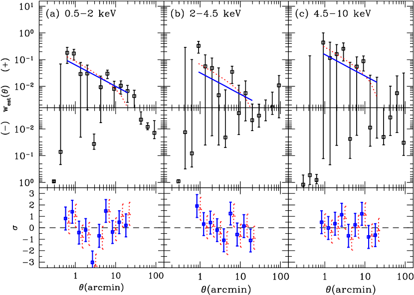
Figure 1: The binned estimated angular correlation functions $w_{\rm est}(\theta)$ are plotted for the X-ray sources detected in the first-year XMM-Newton data in three standard energy bands as labeled. The vertical scale is logarithmic, where the positive and negative parts ($\log|w_{\rm est}(\theta)|>-2.8$ respectively) are attached together. The 1$\sigma$ errors are the diagonal components of Eq. 4, i.e., the scaled random errors. The blue-solid and red-dotted lines (colors in the electronic version only) show the best-fit power-law models for $\gamma-1=0.8$ without and with an integral constraint respectively. The models are plotted in the range where the fits are made. Fit residuals in terms of $\sigma$ has been also plotted in the lower panels for the two models (slightly offset for visibility) in the same line styles (colors) as the models.

3.4 Power-law Fits

In order to make a simple characterization of our ACF results, we have fitted the ACF with a power-law model of the form:

$$w_{\rm mdl}(\theta)=A\;\theta^{1-\gamma}$$

where $\gamma$ is the slope index of the corresponding three-dimensional correlation function. We use the normalization $A$ as a fitting parameter rather than the angular correlation length $\theta_{\rm c}=A^{1/(\gamma-1)}$, since this gives much better convergence of the fit.

The fits are made by minimizing $\chi_{\rm c}^{2}$. The subscript ${\rm c}$ denotes that the correlations between errors have been taken into account through the inverse of the covariance matrix:

$$\chi_{\rm c}^{2}={\bf\Delta}^{\rm T}\,{\bf M}_{\rm cov}^{-1}{\bf\Delta},$$ (5)

where ${\rm\Delta}$ is a vector composed of $w_{\rm est}(\theta_{i})-w_{\rm mdl}(\theta_{i})+C$, $M_{\rm cov}$ is the covariance matrix calculated in Eq. 4 with $N_{\rm run}=80$, and $C$ is a constant to compensate for the integral constraint as discussed below.

Due to the finite area and the construction of $w_{\rm est}$ in Eq. 2, the estimated angular correlation function satisfies the integral constraint (e.g Basilakos et al., 2005; Roche & Eales, 1999):

$$\int\int w_{\rm est}d^{2}\Omega=0.$$ (6)

This constraint usually results in $w_{\rm est}$ underestimating the true underlying angular correlation function by the constant $C$. Under an assumption that the true underlying $w(\theta)$ is a power-law and is extended to the scale of the survey area, one can include $C$ in the fitting process, where $C$ can be uniquely determined by $\theta_{\rm c}$ and $\gamma$ by imposing the integral constraint (Roche & Eales, 1999),

$$C=\sum_{i}A\theta_{i}^{1-\gamma}\,RR(\theta_{i})/\sum_{i}RR(\theta_{i}),$$ (7)

where the sums are over angular bins and $RR(\theta_{i})$ is the number of random-random pairs in the $i$-th angular bin. The above assumption is not necessarily true. If residual systematic errors in the sensitivity maps are the main cause of the negative values at large angular separations, the determination of $C$ shown above is not valid. However, this gives an approximate estimate of the degree of the underestimation by the integral constraint. This sets an limitation to the our angular ACF analysis, where the estimated $C$ values are not negligible compared with the amplitude of the ACF signal. We have made fits with or without including the integral constraint.

Because of the limited signal-to-noise ratio, we were not able to constrain $A$ and $\gamma$ simultaneously. Thus we have calculated the best-fit values and 1$\sigma$ confidence errors for the amplitude for two fixed values of $\gamma-1=0.8$ and $0.5$. The former value is for the canonical value for local galaxies (e.g. Peebles, 1980; Zehavi et al., 2004), the latter is approximately the slope found for X-ray sources in the Chandra Deep Fields (Gilli et al., 2005). The angular fit results are summarized in Table 2. In this table, fits with different bands and parameters are identified with a Fit ID. The angle range for the fits are $\theta_{\rm min}<\theta<\theta_{\rm max}$ and the boundaries are also shown in Table 2. For fit ID’s S1-S4, M1-M4, and U1-U4, we have set $\theta_{\rm min}=0.5\arcmin$ (SFT) or $0.7\arcmin$ (MED,UHD), which is the minimum at which ACF is still positive, and below which the ACF goes negative due to the XMM-Newton PSF. Likewise, we set $\theta_{\rm max}=24\arcmin$, which is about the maximum scale where the ACF is still positive. The best-fit models for $\gamma-1=0.8$ are overplotted in Fig. 1 in the bin ranges included in the fits.

As another choice, we have set $\theta_{\rm min}$ and $\theta_{\rm max}$ in such a way that the range approximately corresponds to the projected comoving distance range of 1-16 $h^{-1}$ Mpc (Fit ID S5,S6,M5,M6,U5, and U6) at the effective median redshift of the sample ($\bar{z}_{\rm eff}$ discussed below in Sect. 4. The rationale for the maximum scale is that, in our subsequent analysis, the correlation functions are converted to the root mean square (rms) density fluctuation with a $8h^{-1}$ Mpc-radius sphere (therefore the relevant maximum separation is $16h^{-1}$) in discussing bias parameters. The rationale for the minimum scale is to minimize the effects of non-linearity in discussing the bias parameters and typical halo masses.

3.5 Effects of Source Merging due to PSF

The amplification bias, due to which the estimated ACF from sources detected in a smoothed image (e.g. by a finite PSF) is amplified with respect to the true underlying ACF, has been first noted and discussed by Vikhlinin & Forman (1995) in the context of the clustering of X-ray sources. This is caused by merging of multiple sources which are separated by distances comparable to or closer than the PSF. The effect of this bias depends on the true underlying angular correlation function and the number density of the sources. In principle, full simulations involving PSF smoothing and the source detection process are required to estimate the amount of this bias. Basilakos et al. (2005) took a simplified approach in estimating this effect on their ACF from their XMM-Newton/2dF survey. In order to estimate the size of the effect, they used particles sampled from a cosmological simulation. They simulated the XMM-Newton sources by merging all the particle pairs closer than $6\arcsec$. They then compared the angular ACFs from the particles themselves and the simulated XMM-Newton sources. As a result, they estimated that the measured angular correlation length is overestimated by 3-4% due to the amplification bias.

In our case with XMM-COSMOS, we have explicitly excluded sources that are classified as extended by the source detection procedure (C06). This causes most of the source pairs closer than $\sim 20\arcsec$ to disappear from the sample, since these pairs are classified as single extended sources. Because the exclusion of these sources can suppress the estimated angular correlation function, we use the term “PSF merging bias” rather than the “amplification bias”. Pairs of sources that are closer than $\sim 4$ arcseconds are, however, detected as a single point source. We have applied a similar approach to Basilakos et al. (2005) in estimating the effects of the PSF merging bias. We have sampled particles from the COSMOS-Mock catalog extracted from the Millennium simulation (Kitbichler, M., priv. comm.) over $\sim 2$ deg² of the sky. Redshift, cosmological intrinsic redshift, and magnitudes in various photometric bands are provided for each mock galaxy in the catalog. We use the mock catalog to estimate the effect of the PSF merging bias in the angular correlation function. Thus the selected objects from the mock catalog for our simulation do not have to physically represent to the actual X-ray selected AGNs. For our present purpose, we have chosen the mock galaxies in a redshift interval (roughly in the range $0.4\lesssim z\lesssim 0.8$) and a magnitude range in such a way that the amplitude of the resulting angular ACF and the source number densities roughly match those of the X-ray samples. We have then created a simulated XMM-COSMOS catalog as follows: 1) source pairs with separations smaller than $4$ arcseconds are merged into single sources and 2) pairs that are between 4 to 20 arcseconds from each other are eliminated. We repeated this experiment 19 times and compared the mean angular ACFs from the original particles and that from simulated XMM-COSMOS by making power-law fits to the mean ACFs. As a result we found that the ACF amplitudes measured using the sources in our source detection procedure on the XMM-COSMOS data are underestimated by 15% and 8% for the SFT and MED bands respectively. Corrections for this effect have not been applied for the values in Table 2, but are considered in further discussions. The effects is negligible in the UHD band, due to the relatively low number density of the sources detected in this band, which made the average distance among neighboring sources much larger than the PSF.

4 Implication for 3-D Correlation Function and Bias

4.1 De-Projection to Real Space Correlation Function

The 2-D ACF is a projection of the real-space 3-D ACF of the sources $\xi(r)$ along the line of sight. In the following discussions and thereafter, $r$ is in comoving coordinates. The relation between the 2-D (angular) ACF and the 3-D ACF is expressed by the Limber’s equation (Peebles, 1980, e.g.,). Under the usual assumption that the scale length of the clustering is much smaller than the distance to the object, this reduces to:

$$w(\theta)N^{2}=\int\left(\frac{dN}{dz}\right)^{2}\times$$

$$\int\xi(\sqrt{[d_{\rm A}(z)\theta]^{2}+l^{2}}\;(1+z)) \left(\frac{dl}{dz}\right)^{-1}dl\;dz,$$ (8)

where $d_{\rm A}(z)$ is the angular distance, $N$ is the total number of sources and $dN/dz$ is the redshift distribution (per $z$) of the sources. The redshift evolution of the 3-D correlation function is customarily expressed by

$$\xi(r,z)=(r/r_{\rm c,0})^{-\gamma}(1+z)^{-3-\epsilon+\gamma},$$ (9)

where $\epsilon=-3$ and $\epsilon=\gamma-3$ correspond to the case where the correlation length is constant in physical and comoving coordinates respectively. In these notations, the zero-redshift 3-D correlation length $r_{\rm c,0}$ can be related to the angular correlation length $\theta_{\rm c}$ by:

$$r_{\rm c,0}^{\gamma}=(N^{2}/S)\,\theta_{\rm c}^{\gamma-1},$$

$$S=H_{\gamma}\int\left(\frac{dN}{dz}\right)^{2}\left(\frac{c\,d\tau(z)}{dz}\right)^{-1}d_{\rm A}^{1-\gamma}(1+z)^{-3-\epsilon}dz$$

$$H_{\gamma}=\frac{\Gamma[(\gamma-1)/2]\Gamma(1/2)}{\Gamma(\gamma/2)},$$ (10)

where $\tau(z)$ is the look back time. Note that all dependence on cosmological parameters are included in $d_{\rm A}(z)$ and $\tau(z)$. We also define the comoving correlation length:

$$r_{\rm c}(\bar{z}_{\rm eff})=r_{{\rm c},0}(1+\bar{z}_{\rm eff})^{(-3-\epsilon+\gamma)/\gamma}$$ (11)

at the effective redshift $\bar{z}_{\rm eff}$, which is the median redshift of the contribution to the angular correlation (the integrand of the second of Eq. 10).

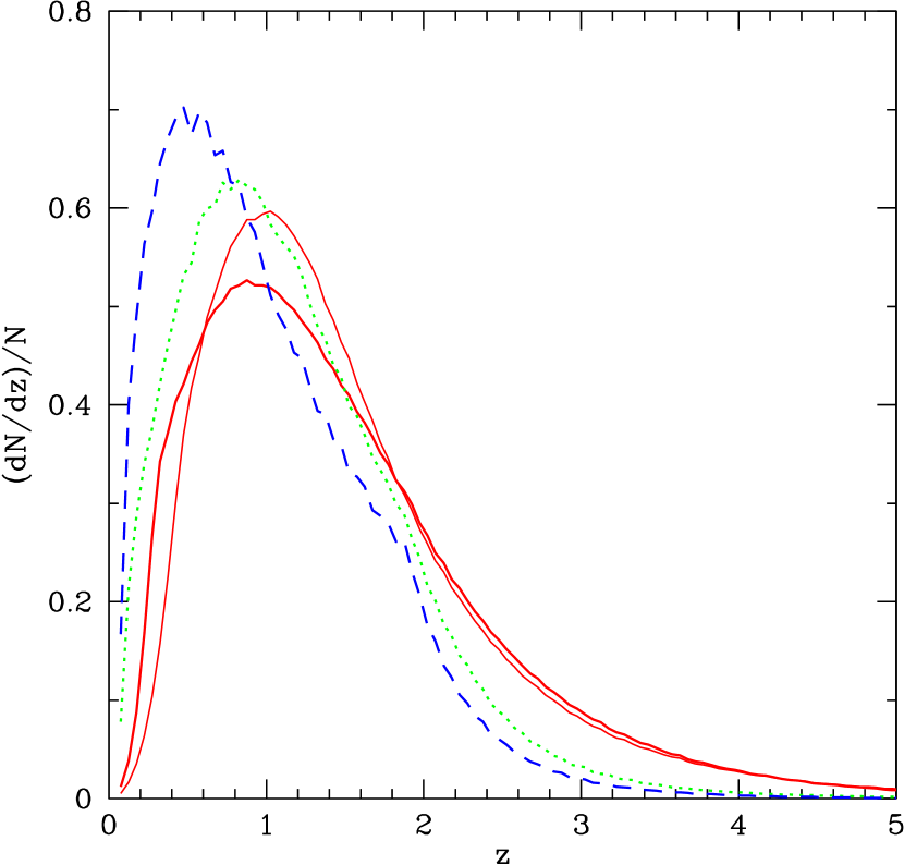
Figure 2: The model redshift distributions of the COSMOS-XMM sources in the 0.5-2 keV (solid lines), 2-4.5 keV (dotted line), and 4.5-10 keV (dashed line) respectively. The thicker and thinner solid lines correspond to the 0.5-2 keV band redshift distributions based on Ueda et al. (2003) model and Hasinger et al. (2005) soft X-ray luminosity function respectively.

An essential ingredient of the de-projection process is the redshift distribution of the sources. At this stage, we do not yet have individual redshifts of a comprehensive set of the XMM-Newton complete sample. Thus we use expected distributions from the X-ray luminosity functions and AGN population synthesis models. We use the model by Ueda et al. (2003) (Luminosity-dependent density evolution or LDDE) for all bands. In calculating the redshift distribution, we have used the sensitivity map in units of CR and the actual XMM-Newton response function in each band. We also use Hasinger et al. (2005) type 1 AGN soft X-ray luminosity function (SXLF) for the 0.5-2 keV for comparison. The redshift distributions of the X-ray sources predicted by these models are plotted in Fig. 4.1. Both Ueda et al. (2003) and Hasinger et al. (2005) used samples with a very high identification completeness with redshifts measurements ($>$ 90%), at least down to the flux limits sampled by the XMM-COSMOS survey. Thus the effect on the expected redshift distribution due to the identification incompleteness is negligible. . In calculating the three dimensional correlation functions, we use the fits with and without integral constraints. The angular correlation amplitude $A$ has been multiplied by a correction factor due to PSF merging as discussed in Sect. 3.5. Also we use the fits with $\gamma=1.8$. The calculated $r_{\rm c,0}$ and the comoving correlation length at the effective median redshift $r_{\rm c}(\bar{z}_{\rm eff})$ are listed in Table 3 for selected results. The errors on $r_{\rm c,0}$ and $r_{\rm c}(\bar{z}_{\rm eff})$ have been calculated for fixed $\gamma$ and $\epsilon$.

4.2 Bias and Comparison with Other Works

In order to estimate the bias parameter of the X-ray sources with respect to the underlying mass distribution, we calculate the rms fluctuation of the distribution of the X-ray sources in the sphere with a comoving radius of $r_{\rm max}=8h^{-1}$ for the power-law model (e.g. §59 of Peebles, 1980),

$$\sigma_{\rm 8,AGN}^{2} =\int\int\xi(|{\bf r_{1}-r_{2}}|)dV_{1}dV_{2}/V^{2}$$ (12)

$$=(r_{\rm max}/r_{\rm c})^{-\gamma}\;J_{2}$$

$$J_{2} =72/[(3-\gamma)(4-\gamma)(6-\gamma)2^{\gamma}].$$ (13)

As discussed above, we have used the results from Fit ID’s S5, S6, M5, M6, U5,and U6, where the fits are made to the angle range corresponding to $\approx$ 1-16 $h^{-1}$ Mpc at $\bar{z}_{\rm eff}$. The corresponding quantity of the underlying mass distribution at $z=0$, $\sigma_{8}$ is one of the commonly used parameters in cosmology (Spergel et al., 2003). In order to compare our results with other similar works on a common ground, we calculated $\sigma_{\rm 8,AGN}$ from power-law representations from literature and plotted them versus the effective redshift of each sample.

For this comparison, we have used the best fit correlation lengths and slopes ($r_{\rm c},\gamma$) from literature to estimate $\sigma_{\rm 8,AGN}$ values and their 1$\sigma$ errors. Since each reference has a different method of presenting results, we take the following strategy in calculating $\sigma_{\rm 8,AGN}$ and its 1$\sigma$ error.

1. If the referenced article gives confidence contours in the ($r_{\rm c},\gamma$) space, we calculate $\sigma_{\rm 8,AGN}$ values for the nominal case as well as at each point in the $L=L_{\rm min}+1$ contour, where $L$ (with the best-fit value $L_{\rm min}$) is either $\chi^{2}$ or a statistical estimator that varies as $\chi^{2}$, e.g. Cash C-estimator for Yang et al. (2006). The error range on $\sigma_{\rm 8,AGN}$ is determined by the minimum and maximum values calculated from the points along the contour.

2. If no confidence contour in the ($r_{\rm c},\gamma$) space is given and there is a fit result with a fixed $\gamma$, we use this fit to calculate $\sigma_{\rm 8,AGN}$. The 1$\sigma$ error in $r_{\rm c}$ is propagated from that of $r_{\rm c}$.

3. If the article gives only best-fit ($r_{\rm c},\gamma$) values, and 1$\sigma$ errors on both parameters, the error of $\sigma_{\rm 8,AGN}$ has been propagated from those of $r_{\rm c}$ and $\gamma$, neglecting possible correlation of errors between these two parameters. In this case, we may well have over/under estimated the errors on $\sigma_{\rm 8,AGN}$.

If the ($r_{\rm c},\gamma$) values are given in multiple evolution models, we use the one where the correlation length is fixed in the comoving coordinates (i.e. $\epsilon=-3-\gamma$). At about the effective median redshift of the sample, however, the correlation lengths calculated assuming different values of $\epsilon$ do not differ significantly. In the case of our present work, we see this by comparing the $r_{\rm c}(\bar{z}_{\rm eff})$ values for $\epsilon=-1.2$ and $\epsilon=-3$ cases in Table 3. Also the value of $\sigma_{\rm 8,AGN}$ is insensitive to the assumed value of $\gamma$. The change of $\sigma_{\rm 8,AGN}$ is less than 0.1 between the assumed $\gamma$ of 1.8 and 1.5 for our results in all the three bands. The results from literature we use for this comparison and the details of the conversion to $\sigma_{\rm 8,AGN}$ are described below, roughly in order of redshift.

Grazian et al. (2004) calculated the correlation function of 392 optically-selected QSOs from the Asiago-ESO/RASS QSO Survey (AERQS) with $\bar{z}_{\rm eff}=0.062$. They found the nominal values of $r_{\rm c}=8.6\pm 2.0\,h^{-1}$ with $\gamma=1.56$. Also in the low-redshift end, Akylas et al. (2000) calculated the correlation function of X-ray selected AGNs from the ROSAT All-Sky Survey (RASS) with a median redshift of $\bar{z}=0.15$. Their correlation length for $\gamma=1.8$ of $r_{\rm c}=6.5\pm 1.0\,h^{-1}$ Mpc for the Einstein de-Sitter Universe is increased by 5% to convert it to our adopted cosmology. Mullis et al. (2004) found $r_{\rm c}=7.4^{+1.8}_{-1.9}\,h^{-1}$ Mpc for $\gamma=1.8$ in their ROSAT North Ecliptic Pole Survey (NEPS) AGNs with median redshift for the contribution to the clustering signal of $\bar{z}_{\rm eff}=0.22$. Basilakos et al. (2004, 2005) in their 2 deg² XMM-Newton survey, with shallower flux limits than XMM-COSMOS, found $r_{\rm c}=16.4\pm 1.3\,h^{-1}$ at $\bar{z}=1.2$ and $r_{\rm c}=19\pm 3\,h^{-1}$ at $\bar{z}=0.75$ for the 0.5-2 and 2-8 keV respectively. A recent work by Puccetti et al. (2006) on the central $\sim 0.6$ deg² region of the ELAIS-S1 field , covered by four mosaiced XMM-Newton exposures with $\sim 50-60$ ks each, also measured angular ACFs of X-ray point sources. For fixed $\gamma=1.8$, they found $r_{\rm c}=12.8\pm 4.2\,h^{-1}$ at $\bar{z}=1.0$ and $r_{\rm c}=17.9\pm 4.8\,h^{-1}$ at $\bar{z}=0.85$ for the 0.5-2 and 2-10 keV bands respectively.

The correlation functions on the deepest X-ray surveys on the Chandra Deep Fields- South (CDF-S; $\bar{z}=0.84$) and North (CDF-N; $\bar{z}=0.96$) by Gilli et al. (2005) gave, for fixed $\gamma=1.4$, $r_{\rm c}=10.4\pm 0.8\,h^{-1}$ and $5.1^{+0.4}_{-0.5}\,h^{-1}$ Mpc respectively. We use the results from their AGN samples. For all of the above samples, the errors on the $\sigma_{\rm 8,AGN}$ have been calculated using method (b).

An extensive redshift-space correlation function was made by Yang et al. (2006), who made use of the data from a combination of the CLASXS and CDF-N surveys, with a significant portion of the X-ray sources having measured spectroscopic redshifts. We have used their ($s_{0},\gamma$) confidence contours, where $s_{0}$ is the redshift-space comoving correlation length, in the four redshift bins with median redshifts of $\bar{z}=$ 0.45, 0.92, 1.26, and 2.07 to estimate $\sigma_{\rm 8,AGN}$ using method (a). In this conversion, we have corrected for the redshift distortion by dividing the redshift-space $\sigma_{\rm 8,AGN}$ value by $\sqrt{1.3}$ (Marinoni et al., 2005; Yang et al., 2006). Extensive clustering studies of QSOs from the 2dF QSO redshift survey (2QZ) have been made using both the projected-distance correlation function approach (Porciani et al., 2004) and the redshift-space three-dimensional correlation function approach (Croom et al., 2005). We have converted the nominal $r_{\rm 0}$–$\gamma$ values and confidence contours in three redshift bins at $\bar{z}_{\rm eff}$=1.06, 1.51 and 1.89 by Porciani et al. (2004) to $\sigma_{\rm 8,AGN}$ using method (a). In converting the Croom et al. (2005)’s ($s_{0},\gamma$) results in 10 redshift bins ranging from $z=0.5$ to 2.5, we have used method c) and the redshift distortion correction has been made in the same way as we have done to the Yang et al. (2006) results.

Figure 3(a) shows the $\sigma_{\rm 8,AGN}$ values as a function of the look back time $\tau(z)$ for our default cosmology from our analysis results both without and with integral constraints. We also overplot $\sigma_{\rm 8,AGN}$ values calculated from the results found in literature as detailed above. In order to compare them with those of the underlying mass distribution, we have also plotted the $\sigma_{\rm 8}\,D(z)$ values from the linear theory (e.g. Carroll et al., 1992; Hamilton, 2001), normalized to 0.75 at z=0 (Spergel et al., 2003) . This curve has been shown to accurately represent the distribution of dark matter particles in the $\Lambda$CDM Hubble Volume Simulation (Marinoni et al., 2005). Figure 3(b) shows the inferred bias parameters $b_{\rm AGN}=\sigma_{\rm 8,AGN}(z)/[\sigma_{8}\,D(z)]$. The values of $\sigma_{\rm 8,AGN}$ and $b_{\rm AGN}$ from this work are shown in Table 4.

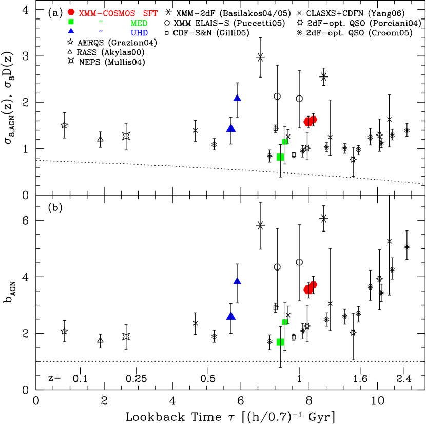
Figure 3: (a) The $\sigma_{\rm 8,AGN}$ of the X-ray sources/AGNs inferred by the power-law fits to the correlation functions from this work and literature are plotted against the look back time corresponding to the effective median redshift of the samples. All error bars indicate 1$\sigma$ errors. The results from this work for the fits without integral constraints are plotted with large solid symbols as labeled (with colors in the electronic version). Those with integral constraints are also plotted with smaller symbols and at positions slightly shifted rightward for visibility. The $\sigma_{\rm 8,AGN}$ values calculated from various results in literature (see text) are also shown as labeled (abbreviated as the first author followed by the last two digits of the publication year). The dotted line shows $\sigma_{8}\,D(z)$ for the mass in the linear theory normalized to 0.9 at z=0. (b) The bias parameter $b_{\rm AGN}=\sigma_{\rm 8,AGN}(z)/[\sigma_{8}\,D(z)]$ are plotted as a function of the effective redshift. The meaning of the symbols are the same as panel (a). We also show redshift ticks at the bottom part of the figure.

5 Discussion and Prospects

In this work, we used all the point sources above the scaled sensitivity threshold without further classification of the sources. We analyzed our results assuming that all the X-ray sources are AGNs. This, in practice, is a good approximation. Our preliminary identifications of the sources indicate that out of the 1037, 545, and 151 sources selected for the ACF analysis for the SFT, MED and UHD bands, 20, 5, and 1 are apparent Galactic stars respectively. Removing these sources from the analysis changed the results very little. Also our results are not likely to be heavily affected by the contamination of clusters/groups, since these sources are extended by $\gtrsim 20\arcsec$ (e.g. Finoguenov et al., 2007) and are likely to be classified as extended by the source detection procedure, hence removed from our sample.

As seen in Fig. 3, with an exception of the MED band, our analysis without integral constraints gives somewhat larger $\sigma_{\rm 8,AGN}$ values than those obtained from results using 2dF optically selected QSOs by Porciani et al. (2004) and Croom et al. (2005), but in general agreement with the values from Chandra CLASXS+CDF-N by Yang et al. (2006), CDF-S by Gilli et al. (2005), and XMM-Newton results from Puccetti et al. (2006). Most likely due to the cosmic variance over a small FOV, Gilli et al. (2005)’s result on CDF-N gave a significantly smaller correlation amplitude than their own CDF-S values as well as our results. The angular ACFs from a shallower XMM-Newton survey by Basilakos et al. (2004, 2005) gave significantly larger $\sigma_{\rm 8,AGN}$ values than other works in both 0.5-2 keV and 2-8 keV bands. The reason for their distinctively large value is unclear.

One of the interesting questions in investigating clustering properties of X-ray selected AGNs is to investigate whether there is any difference in the environments of obscured and unobscured AGNs. Applying the population synthesis model of Ueda et al. (2003) to our sensitivity maps, only $\sim 17$% of the sources detected in the SFT band at $z\sim 1$ are obscured AGNs with $N_{\rm H}>10^{22}$ cm^-2. The fraction increases to $\sim 40$% in the MED and UHD bands. A comparison of bias parameters between SFT band and MED band, which have similar $\bar{z}_{\rm eff}$ values, seems to show a lager bias parameter for the SFT sample. However, with the combination of statistical uncertainties and uncertainties in modeling the integral constraint in the MED band, we can only conclude that the bias of the obscured AGNs is not stronger than that of unobscured AGNs. In other works, Gilli et al. (2005); Yang et al. (2006) as well as Basilakos et al. (2004, 2005) did not find any statistical difference between the clustering properties of these two. Further studies involving the second-year XMM-COSMOS data, which in effect doubles the XMM-Newton exposure over the COSMOS field, and redshift information of individual objects will probe into this problem further. Also with the accepted C-COSMOS program totaling 1.8 Ms of Chandra exposure, we will be able to probe the correlation functions to a much smaller scale, enabling us to investigate the immediate neighbor environments of these AGNs.

Our measured bias parameters based on the rms fluctuations in the 8$h^{-1}$ Mpc radius sphere are in the range $b_{\rm AGN}=1.5-4$. The clustering properties of dark matter halos (DMH) depend on their mass (Mo & White, 1996; Sheth et al., 2001) and we can estimate the typical mass of the DMHs in which the population of AGNs represented by our sample reside, under the assumption that the typical mass halo is the main cause of the AGN biasing. Following the approach of Yang et al. (2006) and Croom et al. (2005) who utilized the model by Sheth et al. (2001), we roughly estimate that the typical mass of DMH is $\sim 10^{13}-10^{14}$ $M_{\sun}$ for our SFT and UHD samples (see Table 4). These are an order of magnitude larger than those estimated by Porciani et al. (2004) and Croom et al. (2005), probably reflecting the large bias parameters from our results.

One of the largest uncertainties in our analysis lies in the treatment of the integral constraint, because its effect is not negligible in our case compared with the ACF amplitudes in the range of our interest. Fig. 3 shows that our results based on the fits with integral constraint, under an assumption that the fitted power-law behavior of the underlying $w(\theta)$ extends to the scale of the entire FOV, give a somewhat larger correlation amplitudes. This assumption may not be true. Also the apparent negative $w_{\rm est}(\theta)$ values at $\theta>30^{\arcmin}$ in Fig. 1 may well be caused by remaining systematic errors. Thus the interpretation of the angular correlation functions, where the signals are diluted by the projection along the redshift space, has a major limitation in correctly taking the integral constraint into account.

The situation will improve when redshift information on individual X-ray sources becomes available for a major and comprehensive set of the X-ray sources. This will enable us to calculate three-dimensional correlation functions or projected-distance correlation functions in a number of redshift bins. With the line-of-sight dilution effect suppressed, we will be able to obtain a larger amplitude in the correlation signal, making the analysis much less subject to the uncertainties in the integral constraint. With optical followup programs underway on the COSMOS field through Magellan and zCOSMOS projects (Trump et al., 2007; Lilly et al., 2006), we are obtaining spectroscopic redshifts from a major fraction of the X-ray sources. At the time of writing this paper, we have been able to define a sample of 378 XMM-COSMOS detected AGNs with measured spectroscopic redshifts ($\sim 30$% of the X-ray point sources), with a median redshift of $z\sim 1$. Our preliminary analysis of these sources based on the projected-distance correlation function $w(r_{\rm p})$ gives a comoving correlation length of $r_{\rm c}\approx 8h^{-1}$ Mpc and $\gamma=1.6$, which is fully consistent with our results without the integral constraints. The results of a full analysis utilizing the redshift information will be presented in a future paper (Gilli et al. in preparation).

Extensive multi-wavelength coverage and the availability of a galaxy catalog also enables us to investigate the cross-correlation function between X-ray selected AGNs and galaxies. By cross-correlating the X-ray selected AGNs with three orders of magnitude larger number of galaxies, we will be able to investigate the environments of the AGN activity in various redshifts with much better statistics.

6 Conclusions

We have presented the first results on the angular correlation functions (ACFs) of the X-ray selected AGNs from the XMM-COSMOS survey and reached the following conclusions.

1. A significant positive angular clustering signals has been detected in the 0.5-2 (SFT) bands in the angle range of $0\farcm 5$-20$\arcmin$, while in the 2-4.5 (MED) and 4.5-10 keV (UHD) bands, the positive signals are 2 and 3$\sigma$ respectively. The robustness of the estimated correlation functions has been verified using different methods of generating random samples.

2. Power-law fits to the angular correlation function have been made, taking into account the correlation of errors. Correctly taking the integral constraint into account is a major limitation on interpreting the angular correlation function. For fits with fixed $\gamma-1=0.8$ and without (with) the integral constraint term, we found correlation lengths of $\theta_{\rm c}=1\farcs 9\pm 0\farcs 3$, $0\farcs 8^{+0\farcs 5}_{-0\farcs 4}$ and $6\arcsec\pm 2\arcsec$ ($3\farcs 1\pm 0\farcs 5$, $2\farcs 2\pm 1\farcs 0$, and $14\arcsec\pm 5\arcsec$) for the SFT, MED, and UHD bands respectively.

3. Due to XMM-Newton PSF, most of the source pairs closer than $\sim 20\arcsec$ are classified as single extended sources, and therefore excluded from the sample. This causes a bias in angular correlation function measurements. We have estimated this effect (the PSF merging bias) by simulations and found that the estimated ACF underestimates the amplitude of the true underlying ACF by $\sim 15$% and $\sim 8$% for the SFT and MED bands respectively

4. Using Limber’s equation and the expected redshift distributions of the sources, we have found comoving correlation lengths of $r_{\rm c}\approx 9.8\pm 0.7$, $5.8^{+1.4}_{-1.7}$, and $12\pm 2$ $h^{-1}$ Mpc for $\gamma=1.8$ at the effective redshifts of $\bar{z}_{\rm eff}\approx$ 1.1, 0.9, and 0.55 for the SFT, MED, and UHD bands respectively for the fits without integral constraints, while 20%-90% larger correlation lengths have been obtained for the fits with integral constraints.

5. Using the fits in the angles corresponding to a projected distance range of 1-16$h^{-1}$ Mpc at the effective median redshift of the sample, we have calculated the rms fluctuations of the X-ray source distributions. Comparing them with that of the mass distribution from the linear theory, we find that the bias parameters of the X-ray sources are in the range $b_{\rm AGN}=1.5-4$ at $0.5<z<1.2$.

6. If the bias mainly reflects the typical mass of dark matter halos in which these X-ray AGNs reside, their typical masses are $10^{13}-10^{14}$ $M_{\sun}$.

7. Further investigations utilizing redshifts of individual X-ray sources and/or involving cross-correlation function with galaxies taking advantage of the wealth of multiwavelength data are being conducted. The approved Chandra observations (C-COSMOS) on this field will enable us to probe into the clustering in much smaller scales and therefore into immediately neighboring environments of AGNs.

Table 1: X-ray sources and Sensitivity limits

Band	Number	$CR_{\rm lim,min}$–$CR_{\rm lim,max}$	$S_{\rm x,lim}$ range	Area
(keV)		(cts s-1)	(erg s-1 cm-2)	(deg-2)
SFT	1037	$7.0\;10^{-4}$–$2.2\;10^{-2}$	$6.7\;10^{-16}$–$2.1\;10^{-14}$	1.43
MED	545	$7.0\;10^{-4}$–$2.5\;10^{-2}$	$4.6\;10^{-15}$–$1.6\;10^{-13}$	1.56
UHD	151	$9.0\;10^{-4}$–$2.2\;10^{-2}$	$8.7\;10^{-15}$–$1.8\;10^{-13}$	1.25

Table 2: Results of the Power-law fits

Fit ID	Band	$A$	$\gamma-1$	$\theta_{\rm c}$	$C$	$\theta_{\rm min}$	$\theta_{\rm max}$
	(keV)	(arcmin1/(γ-1))		(″)		(′)	(′)
S1	SFT	$0.063\pm.008$	$0.8$	$1.9\pm 0.3$	0	0.5	24
S2	SFT	$0.093\pm.012$	$0.8$	$3.1\pm 0.5$	$8\;10^{-3}$	0.5	24
S3	SFT	$0.034\pm.004$	$0.5$	$0.07\pm.02$	0	0.5	24
S4	SFT	$0.078\pm.010$	$0.5$	$0.37\pm.09$	1.5$\;10^{-2}$	0.5	24
S5	SFT	$0.059\pm.009$	$0.8$	$1.7\pm 0.3$	0	1.6	24
S6	SFT	$0.089\pm.015$	$0.8$	$2.9\pm 0.6$	$7\;10^{-3}$	1.6	24
M1	MED	$0.032\pm.015$	$0.8$	$0.8^{+0.5}_{-0.4}$	0	0.7	24
M2	MED	$0.071\pm.027$	$0.8$	$2.2\pm 1.0$	5$\;10^{-3}$	0.7	24
M3	MED	$0.013\pm.008$	$0.5$	$.010^{+.016}_{-.009}$	0	0.7	24
M4	MED	$0.048\pm.020$	$0.5$	$.14^{+.14}_{-.09}$	9$\;10^{-3}$	0.7	24
M5	MED	$0.021\pm.016$	$0.8$	$.47^{+.49}_{-.40}$	0	1.6	24
M6	MED	$0.044\pm.029$	$0.8$	$1.2^{+1.1}_{-0.9}$	3$\;10^{-3}$	1.6	24
U1	UHD	$0.15\pm.05$	$0.8$	$5.6\pm 2.3$	0	0.5	24
U2	UHD	$0.32\pm.09$	$0.8$	$14\pm$ 5	3$\;10^{-2}$	0.7	24
U3	UHD	$0.075\pm.024$	$0.5$	$0.34^{+0.25}_{-0.18}$	0	0.7	24
U4	UHD	$0.23\pm.07$	$0.5$	$3.2^{+2.2}_{-1.6}$	5$\;10^{-2}$	0.7	24
U5	UHD	$0.080\pm.032$	$0.8$	$2.5^{+1.3}_{-1.2}$	0	2.4	35
U6	UHD	$0.17\pm.06$	$0.8$	$6.5^{+3.0}_{-2.7}$	3$\;10^{-2}$	2.4	35

Table 3: Three Dimensional Correlation Lengths

Fit ID	$\gamma$	$\epsilon$	$\bar{z}_{\rm eff}$	$r_{\rm c,0}$	$r_{\rm c}(\bar{z}_{\rm eff})$	Model
				[$h^{-1}$ Mpc]
S1	1.8	-1.2	1.07	9.8$\pm 0.7$	9.8$\pm 0.7$	U03
S1	1.8	-1.2	1.11	9.4$\pm 0.7$	9.4$\pm 0.7$	H05
S1	1.8	-3.0	1.42	4.3$\pm 0.3$	10.4$\pm 0.7$	U03
S2	1.8	-1.2	1.07	12.1$\pm 0.9$	12.1$\pm 0.9$	U03
S5	1.8	-1.2	1.07	9.4$\pm 0.8$	9.4$\pm 0.8$	U03
S6	1.8	-1.2	1.07	11.8$\pm$1.1	11.8$\pm$1.1	U03
M1	1.8	-1.2	0.87	5.8${}^{+1.4}_{-1.7}$	5.8${}^{+1.4}_{-1.7}$	U03
M1	1.8	-3.0	1.13	2.9${}^{+0.7}_{-0.8}$	6.1${}^{+1.5}_{-1.8}$	U03
M2	1.8	-1.2	0.87	9.0${}^{+1.8}_{-2.1}$	9.0${}^{+1.8}_{-2.1}$	U03
M5	1.8	-1.2	0.87	4.6${}^{+1.7}_{-2.5}$	4.6${}^{+1.7}_{-2.5}$	U03
M6	1.8	-1.2	0.87	6.9${}^{+2.2}_{-3.1}$	6.9${}^{+2.2}_{-3.1}$	U03
U1	1.8	-1.2	0.60	11.9${}^{+2.1}_{-2.4}$	11.9${}^{+2.1}_{-2.4}$	U03
U1	1.8	-3.0	0.88	6.6${}^{+1.1}_{-1.2}$	12.5${}^{+2.2}_{-2.5}$	U03
U2	1.8	-1.2	0.60	19$\pm 3$	19$\pm 3$	U03
U5	1.8	-1.2	1.60	8.4${}^{+1.7}_{-2.0}$	8.4${}^{+1.7}_{-2.0}$	U03
U6	1.8	-1.2	1.60	12.7${}^{+2.3}_{-2.7}$	12.7${}^{+2.3}_{-2.7}$	U03

Table 4: Estimated $\sigma_{\rm 8,AGN}$ and Bias

Fit ID	$\bar{z}_{\rm eff}$	$\sigma_{\rm 8,AGN}$	$b_{\rm AGN}$	$\log M_{\rm halo}$
				$h^{-1}\,M_{\sun}$
Without integral constraint…
S5	1.07	1.58${}^{+.12}_{-.13}$	3.5$\pm$0.3	13.6$\pm 0.1$
M5	0.87	0.82${}^{+.27}_{-.42}$	1.7${}^{+0.6}_{-0.9}$	$<$13.3
U5	0.60	1.42${}^{+.26}_{-.32}$	2.6${}^{+0.5}_{-0.6}$	13.5$\pm 0.2$
With integral constraint…
S6	1.07	1.63${}^{+.13}_{-.14}$	3.7$\pm$0.3	13.6$\pm$0.1
M6	0.87	1.19${}^{+.34}_{-.50}$	2.5${}^{+0.7}_{-1.0}$	13.3${}^{+0.3}_{-0.7}$
U6	0.60	2.08${}^{+.34}_{-.41}$	3.8${}^{+0.6}_{-0.8}$	13.9$\pm 0.2$

References

- Akylas et al. (2000) Akylas, A., Georgantopoulos, I., & Plionis, M. 2000, MNRAS, 318, 1036
- Barger et al. (2005) Barger, A. J., Cowie, L. L., Mushotzky, R. F., Yang, Y., Wang, W.-H., Steffen, A. T., & Capak, P. 2005, AJ, 129, 578
- Basilakos et al. (2004) Basilakos, S., Georgakakis, A., Plionis, M., & Georgantopoulos, I. 2004, ApJ, 607, L79
- Basilakos et al. (2005) Basilakos, S., Plionis, M., Georgakakis, A., & Georgantopoulos, I. 2005, MNRAS, 356, 183
- Brusa et al. (2007) Brusa, M. et al. 2006, ApJS, this volume
- Budavári et al. (2003) Budavári, T., et al. 2003, ApJ, 595, 59
- Cappelluti et al. (2005) Cappelluti, N., Cappi, M., Dadina, M., Malaguti, G., Branchesi, M., D’Elia, V., & Palumbo, G. G. C. 2005, A&A, 430, 39
- Cappelluti et al. (2007) Cappelluti, N. et al. 2006, ApJS, this volume (C07)
- Cappi et al. (2001) Cappi, M., et al. 2001, ApJ, 548, 624
- Carroll et al. (1992) Carroll, S. M., Press, W. H., & Turner, E. L. 1992, ARA&A, 30, 499
- Comastri et al. (1995) Comastri, A., Setti, G., Zamorani, G., & Hasinger, G. 1995, A&A, 296, 1
- Croom et al. (2005) Croom, S. M., et al. 2005, MNRAS, 356, 415
- D’Elia et al. (2004) D’Elia, V., Fiore, F., Elvis, M., Cappi, M., Mathur, S., Mazzotta, P., Falco, E., & Cocchia, F. 2004, A&A, 422, 11
- Di Matteo et al. (2005) Di Matteo, T., Springel, V., & Hernquist, L. 2005, Nature, 433, 604
- Finoguenov et al. (2007) Finoguenov, A. et al. 2006, ApJS, this volume
- Gilli et al. (2001) Gilli, R., Salvati, M., & Hasinger, G. 2001, A&A, 366, 407
- Gilli et al. (2003) Gilli, R., et al. 2003, ApJ, 592, 721
- Gilli et al. (2005) Gilli, R., et al. 2005, A&A, 430, 811
- Grazian et al. (2004) Grazian, A., Negrello, M., Moscardini, L., Cristiani, S., Haehnelt, M. G., Matarrese, S., Omizzolo, A., & Vanzella, E. 2004, AJ, 127, 592
- Hamilton (2001) Hamilton, A. J. S. 2001, MNRAS, 322, 419
- Hasinger et al. (2005) Hasinger, G., Miyaji, T., & Schmidt, M. 2005, A&A, 441, 417
- Hasinger et al. (2007) Hasinger, G. et al. 2006, ApJS, this volume
- La Franca et al. (2005) La Franca, F., et al. 2005, ApJ, 635, 864
- Landy & Szalay (1993) Landy, S. D., & Szalay, A. S. 1993, ApJ, 412, 64
- Lilly et al. (2006) Lilly, S. J. et al. 2006, ApJS, this volume
- Marinoni et al. (2005) Marinoni, C., et al. 2005, A&A, 442, 801
- Menci et al. (2004) Menci, N., Fiore, F., Perola, G. C., & Cavaliere, A. 2004, ApJ, 606, 58
- Miyaji, Hasinger & Schmidt (2000) Miyaji, T., Hasinger, G. & Schmidt, M. 2000, A&A 353, 25
- Mo & White (1996) Mo, H. J., & White, S. D. M. 1996, MNRAS, 282, 347
- Moretti et al. (2003) Moretti, A., Campana, S., Lazzati, D., & Tagliaferri, G. 2003, ApJ, 588, 696
- Mullis et al. (2004) Mullis, C. R., Henry, J. P., Gioia, I. M., Böhringer, H., Briel, U. G., Voges, W., & Huchra, J. P. 2004, ApJ, 617, 192
- Peebles (1980) Peebles, P. J. E., 1980, The Large Scale Structure of the Universe (Princeton:Princeton Univ. Press)
- Porciani et al. (2004) Porciani, C., Magliocchetti, M., & Norberg, P. 2004, MNRAS, 355, 1010
- Puccetti et al. (2006) Puccetti, S., Fiore, F., D’Elia, V. et al., A&A, submitted
- Roche & Eales (1999) Roche, N., & Eales, S. A. 1999, MNRAS, 307, 703
- Scoville et al. (2007) Scoville, N. et al. 2006, ApJS, this volume
- Sheth et al. (2001) Sheth, R. K., Mo, H. J., & Tormen, G. 2001, MNRAS, 323, 1
- Spergel et al. (2003) Spergel, D. N., et al. 2003, ApJS, 148, 175
- Trump et al. (2007) Trump, R.J. et al. 2006, ApJS, this volume
- Ueda et al. (2003) Ueda, Y., Akiyama, M., Ohta, K. & Miyaji, T. 2003, ApJ 598, 886
- Vikhlinin & Forman (1995) Vikhlinin, A., & Forman, W. 1995, ApJ, 455, L109
- Yang et al. (2003) Yang, Y., Mushotzky, R. F., Barger, A. J., Cowie, L. L., Sanders, D. B., & Steffen, A. T. 2003, ApJ, 585, L85
- Yang et al. (2006) Yang, Y., Mushotzky, R. F., Barger, A. J., & Cowie, L. L. 2006, ApJ in press (astro-ph/0601634)
- Zehavi et al. (2004) Zehavi, I., et al. 2004, ApJ, 608, 16