Multiscale Methods

Bernard Jones told you about multiresolution analysis in his wavelet lectures. This is a pretty well formalized and self-contained area of wavelet analysis. Multiscale methods form a wider and less well defined area of tools and approaches; the term is used, e.g., in numerical analysis, but the main range of multiscale methods are based on application of wavelets.

In this this lecture I shall explain how to carry out multiscale morphological analysis of cosmological density fields. For that, we have to use wavelets to decompose the data into different frequency bands, to calculate densities, and to describe morphology.

Let us start with wavelet transforms.

1 Wavelet Transforms

The most popular wavelet transforms are the orthogonal fast transforms, described by Bernard Jones. For morphological analysis, we need different transforms. The easiest way to understand wavelets is to start with continuous wavelet transforms.

1.1 Continuous Wavelet Transform

The basics of wavelets are most easily understood in the case of one-dimensional signals (time series or data along a line). The most commonly used decomposition of such a signal (f(x)) into contributions from different scales is the Fourier decomposition:

$$\hat{f}(k)=\int_{-\infty}^{\infty}f(x)\exp(-{\rm i}\,kx)\,dx\;.$$

The Fourier amplitudes $f(k)$ describe the frequency content of a signal. They are not very intuitive, however, as they depend on the behaviour of a signal as a whole; e.g., if the signal is a density distribution along a line, then all the regions of the universe where this line passes through, contribute to it. Fourier modes are homeless.

For analyzing the texture of images and fields, both scales and positions are important. The right tools for that are continuous wavelets. A wavelet transform of our signal $f(x)$ is

$$W(a,b)=\frac{1}{\sqrt{a}}\int_{-\infty}^{\infty}f(x)\psi\left(\frac{x-b}{a}\right)\,dx\;,$$

where $\psi(x;a,b)$ is a wavelet profile. Here the argument $b$ ties the wavelet to a particular location, and $a$ is the scale factor.

In order to be interesting (and different from the Fourier modes), typical wavelet profiles have a compact support. Two popular wavelets are shown in Fig. 1 – the Morlet wavelet, and the Mexican hat wavelet (see the formulae in Bernard Jones lecture). The Morlet wavelet is a complex wavelet.

Figure 1: Left – Morlet wavelet (solid line shows its real part, dashed line – the imaginary part), right – (a real-valued ) Mexican hat wavelet

Continuous wavelets are good for finding sharp edges and singularities of functions. An example of that is given in Fig. 2. The brightness-coded wavelet amplitudes (mexican-hat wavelet) for the upper-panel skyline show features at all scales.

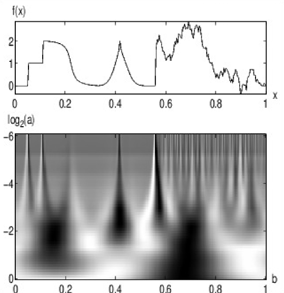
Figure 2: Example (continuous mexican hat wavelet)

This example shows us also the information explosion inherent to continuous wavelets – a function $f(x)$ gives rise to a two-argument wavelet amplitude $W(a,b)$; the collection of continuous wavelet amplitudes is heavily redundant. If the wavelet is well-behaved (2), the wavelet amplitudes can be used to restore the original function:

$$f(x)=\frac{1}{C_{\psi}}\int_{0}^{\infty}\int_{-\infty}^{\infty}\frac{1}{\sqrt{a}}W(a,b)\psi^{\star}\left(\frac{x-b}{a}\right)\frac{da\,db}{a^{2}}\;,$$ (1)

where

$$C_{\psi}=\int_{0}^{\infty}\frac{\hat{\psi}^{\star}(\nu)\hat{\psi}(\nu)}{\nu}d\nu\;$$

($\psi^{\star}$ is a complex conjugate of $\psi$, and $\hat{\psi}$ is the Fourier transform of $\psi$). This constant exists ($C_{\psi}<\infty$), when

$$\hat{\psi}(0)=0\Rightarrow\int_{-\infty}^{\infty}\psi(x)\,dx=0\;.$$ (2)

This is the only requirement that a continuous-transform wavelet has to satisfy. Equation (1) shows that we need to know the wavelet amplitudes of all scales to reconstruct the original function. We also see that large-scale wavelet amplitudes are heavily downweighted in this reconstruction.

1.2 Dyadic Wavelet Transform

It is clear that the information explosion inherent in application of continuous wavelets has to be restrained. The obvious way to proceed is to consider computational restrictions.

First, computations need to be carried out on a discrete coordinate grid $b_{i}$. Second, if we look at Fig. 2 we see that the wavelet amplitudes change, in general, smoothly with scale. This suggests that a discrete grid of scales could suffice to analyze the data. While the obvious choice for the coordinate grid is uniform, the scale grid is usually chosen logarithmic, in hope to better catch the scale-dependent behaviour. This discretisation generates much less data than the continuous transform did, only $N\times J$, where $N$ is the size of the original data (the number of grid points), and $J$ is the number of different scales. The most popular choice of the scale grid is where neighbouring scales differ by a factor of two. Other choices are possible, of course, but this choice is useful in several respects, as we shall see below.

Such a wavelet transform is called dyadic. As we saw above, any compact function with the zero mean could be used as an analyzing wavelet. In the case of a discrete wavelet transform, we, however, have a problem – can we restore the original signal, given all the wavelet amplitudes obtained? It is not clear at first sight, as the restoration integral for a continuous wavelet (1) contains contributions of all wavelet scales.

The answer to that is yes, given that the frequency axis is completely covered by the wavelets of dyadic scales (the wavelets form a so-called frame). This requirement is referred to as the perfect reconstruction condition; I shall show a specific example below.

Let us rewrite now the wavelet transform, for finite grids. As we have heard about the multiresolution analysis already, we shall try to introduce both the smooth and the detail part of the transform. Let the initial data be $a_{0}(m)$ (the index $0$ shows the transform order, and the argument $m$ – the grid point). The smoothing operation and the wavelet transform proper are convolutions, so they can be written

$$a_{j+1}(m)=\sum_{k}h_{j}(k)a_{j}(m+k)\;,\qquad d_{j+1}(m)=\sum_{k}g_{j}(k)a_{j}(m+k)\;,$$ (3)

where the filters $h_{j}(k)$ and $g_{j}(k)$ are different from zero for a few values of $k$ around $0$ only (the wavelet transform is local). Applying recursively this rule, we can find wavelet transforms of all orders, starting from the data ($a_{0}(\cdot)$).

Now, we should like to be able to restore the signal, knowing the $a_{j}(\cdot)$ and $d_{j}(\cdot)$. As the previous filters were linear, restoration should also be linear, and we demand:

$$a_{j}(m)=\sum_{k}\tilde{h}_{j}(k)a_{j+1}(m+k)+\sum_{k}\tilde{g}_{j}(k)d_{j+1}(m+k)\;.$$ (4)

It can be proved that these rules will work for any dyadic wavelet that satisfies the so-called unit gain condition, if the filters are upsampled (see next section).

If you recall (or look up) Bernard Jones’ lecture, you will notice that the rules (3,4) look the same as the rules for bi-orthogonal wavelets. The only difference is that for bi-orthogonal wavelets the filters have to satisfy an extra, so-called aliasing cancellation condition, arising because of the downsampling of the grid.

1.3 À Trous Transform

This downsampling leads us to the next problem. The change of the frequency (scale) between wavelet orders when bi-orthogonal or orthogonal wavelet transforms are used, is achieved by downsampling – choosing every other data point. Applying the same wavelet filter on the downsampled data set is equivalent to using the twice as wide filter on the original data. Now, in our case the grid is not diluted, and all points participate for all wavelet orders. The obvious solution here is to upsample the filter – to introduce zeros between the filter points. This doubles the filter width, and it is also useful for the computational point of view, as the operations count for the convolutions does not depend now on the wavelet order. Because of these zeros (holes), such a dyadic transform is called “à trous” (’with holes’ in French; the transform was introduced by French mathematicians, Holschneider et al. (ESholtz )).

In Fourier language, such an upsampling halves the frequency:

$$\hat{h}_{1}(\omega)=\hat{h}_{0}(2\omega)\;,\qquad\hat{h}_{j}(\omega)=\hat{h}(2^{j}\omega)\;,$$

where $\omega$ stands for the frequency, and $h(k)\equiv h_{0}(k),\hat{h}(\omega)\equiv\hat{h}_{0}(\omega).$ Although we describe localized transforms, it is useful to use Fourier transforms, occasionally – convolutions are frequent in wavelet transforms, and convolutions are converted to simple multiplications in Fourier space. Now, in coordinate space, the explicit expression for the upsampled filter $h(\cdot)$ is:

$$h_{j}(k^{\prime})=h(k)\delta(k^{\prime}-k\cdot 2^{j})\;,$$

saying simply that the only non-zero components of the smoothing filter for the order $j$ are those that have the index $k\cdot 2^{j}$, and they are determined by the original filter values $h(k)\equiv h_{0}(k)$. Let us write now the smoothing sum again:

$$a_{j+1}(m)=\sum_{k^{\prime}}h_{j}(k^{\prime})a_{j}(m+k^{\prime})=\sum_{k}h(k)a_{j}(m+2^{j}k)\;,$$ (5)

where we retained only the non-zero terms in the last sum. The last equality is of the form usually used in à trous transforms; the holes are returned to the data space again. However, the procedure is different from the bi-orthogonal transform, as we find the scaling and wavelet amplitudes for every grid point $m$, not for the downsampled sets only. The wavelet rule with holes reads

$$d_{j+1}(m)=\sum_{k}g(k)a_{j}(m+2^{j}k)\;,$$ (6)

where, obviously, $g(k)\equiv g_{0}(k)$.

Let us now construct a particular à trous transform, starting backwards, from the reconstruction rule (4). In multiresolution language, this rule tells us that the approximation (sub)space $V_{j}$ where the “smooth functions” live, is a direct sum of two orthogonal subspaces of the next order (the formula is for projections, but it follows from this fact). Let us take it in a much simpler way, literally, and demand:

$$a_{j}(m)=a_{j+1}(m)+d_{j+1}(m)\;,$$ (7)

or $\tilde{h}(k)=\tilde{g}(k)=\delta_{0k}\;$. This is a very good choice, as applying it recursively we get

$$a_{0}(m)=a_{J}(m)+\sum_{j=J}^{j=1}d_{j}(m)\;,$$ (8)

meaning that the data is decomposed into a simple sum of contributions of different details (wavelet orders) and the most smooth picture. As there are no extra weights, these detail spaces have a direct physical meaning, representing the life in the full data space at a given resolution.

The condition (7) gives us at once the formula for the wavelet transform

$$d_{j+1}(m)=a_{j}(m)-a_{j+1}(m)=\sum_{k}\left[\delta_{0k}-h(k)\right]a_{j}(m+k)\;,$$ (9)

or $g(k)=\delta_{0k}-h(k)\;$.

So far, so good. Now we have only to choose the filter $h(k)$ to specify the transform. As the filter is defined by the scaling function $\phi(x)$ via the two-scale equation

$$\phi(x/2)=2\sum_{k}h(k)\phi(x-k)\;,$$ (10)

meaning simply that the scaling function of the next order (note that $f(x/2)$ is only half as fast as $f(x)$) has to obey the smoothing rule in (5) exactly (the space where it lives is a subspace of the lower order space). Different normalizations are used; the coefficient 2 appears here if we omit extra coefficients for the convolution (10) in the Fourier space:

$$\hat{\phi}(2\omega)=\hat{h}(\omega)\hat{\phi}(\omega)$$

(recall that the coordinate space counterpart of $\hat{f}(2\omega)$ is $f(x/2)/2$). Obviously, not all functions satisfy the two-scale equation (10), but a useful class of functions that do are box splines.

1.4 Box Splines

Box splines are easy to obtain – an $n$-th degree box spline $B_{n}(x)$ is the result of $n+1$ convolutions of the box profile $B_{0}(x)=1,\quad x\in[0,1]$ with itself. Some authors like to shift it, some not; we adopt the condition that the convolution result is centred at 0 when $n$ is odd, and at $x=1/2$ when $n$ is even. This convention gives a simple expression for the Fourier transform of the spline:

$$\hat{B_{n}}(\omega)=\left(\frac{\sin(\omega/2)}{\omega/2}\right)\exp\left(-{\rm i}\,\varepsilon\omega/2\right)\;,$$ (11)

where $\varepsilon=1$, if $n$ is even, and 0 otherwise. You can easily derive the formula yourselves, recalling that the Fourier transform of a $[-1,1]$ box is the sinc($\cdot$) function, and using the rule for the argument shifts.

Box splines have, just to start, several very useful properties. First, they are compact; in fact, they are the most compact polynomials for a given degree ($B_{n}(x)$ is a polynomial of degree $n$). Second, they are interpolating,

$$\sum_{k}B_{j}(x-k)=1\;,$$ (12)

a necessary condition for a scaling function. And box splines satisfy the two-scale equation (10), with

$$h(k)=2^{-(n+1)}{n\choose k}\;,$$ (13)

where $n$ is the degree of the spline (see de Boor (ESdeboor ). This formula is written for unshifted box splines, and here the index $k$ ranges from 0 to $n$. It is easy to modify (13) for centred splines; e.g., for centred box-splines of an odd degree $n$ the index $k$ ranges from $-(n+1)/2$ to $(n+1)/2$, and we have to replace $k$ at the right-hand side of (13) by $k+(n+1)2$.

I do not intend to be original, and shall choose the $B_{3}$ box spline for the scaling function. This is the most beloved box spline in astronomical community; see, e.g., the monograph by Jean-Luc Starck and Fion Murtagh (ESstarck06 ) for many examples. As any spline, this can be given by different polynomials in different coordinate intervals; fortunately, a compact expression exists:

$$\phi(x)=B_{3}(x)=\frac{1}{12}\left(|x-2|^{3}-4|x-1|^{3}+6|x|^{3}-4|x+1|^{3}+|x+2|^{3}\right)\;.$$ (14)

This function is identically zero outside the interval $[-2,2]$. Formula (13) gives us the filter $h(k)$:

$$h(k)=(1/16,1/4,3/8,1/4,1/16)\;,\qquad k\in[-2,2]\;.$$ (15)

In order to obtain the associated wavelet $\psi(\cdot)$, we have to return to our recipe for calculating the wavelet coefficients (9). These coefficients are, in principle, convolutions (multiplications in Fourier space):

$$\hat{d}_{i+1}(\omega)=\hat{\psi}(\omega)\hat{a}_{i}(\omega)\;,$$ (16)

So, (9) gives us

$$\hat{\psi}(\omega)\hat{a}_{i}(\omega)=\hat{\phi}(\omega/2)\hat{a}_{i}(\omega)-\hat{\phi}(\omega)\hat{a}_{i}(\omega)\;,$$

or,

$$\hat{\psi}(\omega)=\hat{\phi}(\omega/2)-\hat{\phi}(\omega)\;.$$ (17)

For coordinate space, the above expression transforms to

$$\psi(x)=2\phi(2x)-\phi(x)\;.$$ (18)

Figure 3: The $B_{3}$ scaling function ($\phi$) and its associated wavelet ($\psi$)

Both the $B_{3}$ box spline (the scaling function $\phi(x$) and its associated wavelet $\phi(x)$ are shown in Fig. 3.

I cannot refrain from noting that the last exercise was, strictly speaking, unnecessary. We could have proceeded with our wavelet transform after obtaining the filter $h(k)$ (15). But is nice to know the wavelet by face and to get a feeling what our algorithms really do.

Now I can also show you the Fourier transform of the wavelet (17), to reassure you that such a wavelet can be built and that it does not leave gaps in the frequency axis. We see, first, that the filter peaks at $\omega\approx\pi$, giving for its characteristic wavelength $\lambda=2\pi/\omega=2$ (grid units). Second, we see that neighbouring wavelet orders overlap in frequency. The reason for that is that our wavelets are not orthogonal. So we loose a bit in frequency separation, but gain in spatial resolution.

Figure 4: The Fourier transforms of the three subsequent orders of the $B_{3}(\cdot)$-associated wavelet. The transforms fully cover the frequency axis, but the overlap between different orders is substantial

Two points more: first, about normalization. Although our scaling function $\phi(x)$ is normalized in the right way (its integral is 1), the coefficient in the two-scale equation (10 is different from the conventional one, and, as a result, the filter coefficients $h_{k}$ sum to 1, not to $\sqrt{2}$. The integral over the wavelet profile is zero (this ensures that $\psi(x)$ is really a wavelet), but its norm $\int\psi^{2}(x)\,dx\approx 0.2345$; normally it is chosen to be 1. What matters, really, is that it is not zero and does not diverge; welcome to the wavelet world of free normalization.

Second, about initial data. We can recursively apply the transformation rules (5, 6) only if we assume that the data $a_{0}(m)$ belongs to the class of smooth functions (those obtained by convolution with the scaling function). So, if the raw data comes in ticking at grid points (regular times), we should smooth it once before starting our transform chain. If the raw data is given at points $x$ that do not coincide with the grid, the right solution is to distribute it to the grid $m$ with the scaling weights $\phi(x-m)$. This procedure was christened ’extirpolation’ (inverse interpolation) by Press et al. (ESpress ); a strange fact is that N-body people extirpolate all the time in their codes, but nobody wants to use the term.

So, we have specified all the recipes needed to perform the à trous transform. Before we do that, we have to answer the question – why? Bernard Jones demonstrated us how well orthogonal wavelet transforms work. An orthogonal wavelet transform changes a signal (picture) of $N$ pixels into exactly $N$ wavelet amplitudes, while an à trous transform expands it into $N\times J$ pictures; why bother?

The reason is called ’translational invariance’. As many of the wavelet amplitudes of an orthogonal transform do not have an exact home, then, when shifting the data, these amplitudes change in strange ways. Sure, we can always use them to reconstruct the shifted picture, but it makes no sense to compare the wavelet amplitudes of the original and shifted pictures. All the à trous transforms, in the contrary, keep their amplitudes, these move together with the grid. This is ’translational invariance’, and it is important in texture studies, where we want to see different scales of a picture at exactly the same grid point. And cosmic texture is the main subject of this lecture.

A point to note – Fourier transforms are not translation invariant, too.

1.5 Multi-Dimensional À Trous

All the above discussion was devoted to one-dimensional wavelets. This is customary in wavelet literature, as the step into multi-dimensions is simple – we form direct products of independent one-dimensional wavelets, one for every coordinate. This has been the main approach up to now, although it does not work well everywhere. An important example is a sphere, where special spherical wavelets have to be constructed (I suppose that these will be explained in the CMB-lectures).

So, two-dimensional wavelets are introduced by defining the 2-D scaling function

$$\phi(x,y)=\phi(x)\phi(y)\;,$$ (19)

and three-dimensional wavelets – by the 3-D scaling function

$$\phi(x,y,z)=\phi(x)\phi(y)\phi(z)\;.$$ (20)

A little bit extra care has to be taken to define wavelets; we have to step into Fourier space for a while for that. Recalling (17), we have to write for two dimensions

$$\hat{\psi}(\omega_{1},\omega_{2})=\hat{\phi}(\omega_{1}/2)\hat{\phi}(\omega_{2}/2)-\hat{\phi}(\omega_{1})\hat{\phi}(\omega_{2})$$

(the direct products (19, 20) look exactly the same in the Fourier space). For coordinate space, it gives

$$\psi(x,y)=4\phi(2x)\phi(2y)-\phi(x)\phi(y)\;,$$

and for three dimensions, respectively

$$\psi(x,y,x)=8\phi(2x)\phi(2y)\phi(2z)-\phi(x)\phi(y)\phi(z)\;,$$

Figure 5: Two-dimensional $B_{3}$-associated wavelet

I show the $B_{3}$-associated wavelets in Figs. 5 and 6. Because of their definition, the wavelet profiles are symmetric, but not isotropic, right? A big surprise is that both the $B_{3}$ scaling functions and the wavelets are practically isotropic, as the figures hint at. Let us define the isotropic part of the 2-D wavelet as

$$\overline{\psi}(r)=\frac{1}{2\pi}\int_{0}^{2\pi}\psi(r\cos\alpha,r\sin\alpha)\,d\alpha\;,$$

and estimate the deviation from isotropy by

$$\epsilon=\int_{-2}^{2}\int_{-2}^{2}|\psi(x,y)-\overline{\psi}(\sqrt{x^{2}+y^{2}})|\,dx\,dy\;.$$

Comparing $\epsilon$ with the integral over the absolute value of our wavelet itself (about 4/9), we find that the difference is about 2%. For three dimensions, the difference is a bit larger, up to 5%.

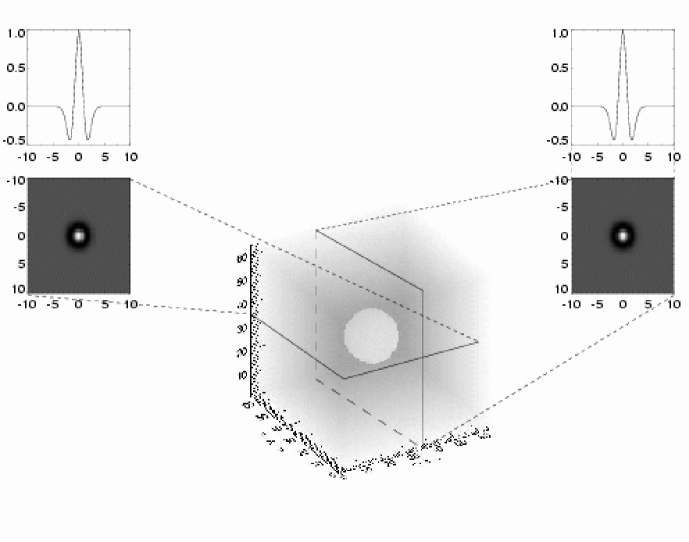
Figure 6: Three-dimensional $B_{3}$-associated wavelet

This isotropy is important for practical applications; it means that our choice of specific coordinate directions does not influence the results we get.

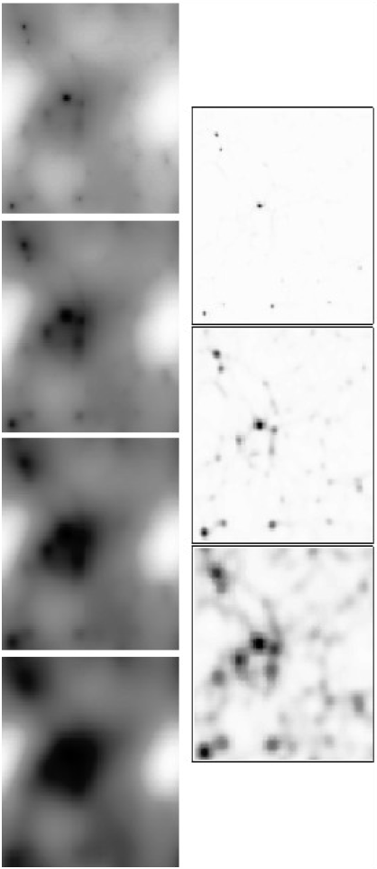
Figure 7: Á trous potential (slices) for a N-body model (linear scale)

And, as an example, I show a sequence of transforms in Fig. 7. Those are slices of a 3-D $B_{3}$-associated à trous transform sequence for the gravitational potential image of a N-body simulation. The data slice is at the upper left; the left column shows the scaling solutions, higher orders up. The right column shows the wavelet amplitudes; the data can be restored by taking the lower left image, and by adding to it all the wavelet images from the right column. Simple, is it?

2 Cosmological Densities

In cosmology, the matter density distribution is a very important quantity that, first, determines the future dynamics of structure, and, second, may carry traces of the very early universe (initial conditions). We, however, cannot observe it. The data we get, after enormous effort, gives us galaxy positions in (redshift) space; even if we learn to associate a proper piece of dark matter with a particular galaxy, we have a point process, not a continuous density field.

There are several ways to deal with that. First, we have to introduce a coordinate grid; an extra discrete entity, but necessary when using continuous fields in practical computations.

2.1 N-Body Densities

A similar density estimation problem arises in N-body calculations. The fundamental building blocks there are mass points; these points are moved around every timestep, and in order to get the accelerations for the next timestep, the positions of the points have to be translated to the mass density on the underlying grid.

The simplest density assignment scheme is called NGP (nearest grid point), where the grid coordinate $i$ is found by rounding the point coordinate $x$ (to keep formulae simple, consider one-dimensional case and grid step one; generalization is trivial). Thus, the NGP assignment law is $i=\mathrm{floor}(x+0.5)$. This scheme is pretty rough, but I have seen people using an even worse scheme, $i=\mathrm{floor}(x)$.

A bit more complex scheme is CIC (cloud in cell) where the mass point is dressed in a cubic cloud of the size of the grid cell, and vertices’s are dressed in a similar region of influence. The part of the cloud that intersects this region of influence is assigned to the vertex. Sounds complicated, but as the mass weights are obtained by integration over the constant-density cloud, it is, in fact, only linear extirpolation (in 3-D, three linear).

The most complex single-cloud scheme used is TSC (triangular shaped cloud), where the density of the cloud changes linearly from a maximum in the centre, to zero at the borders. The mass integration needed ensures that this scheme is quadratic extirpolation.

Note that the last two mass assignment schemes are, if fact, centred $B$-spline assignments – the vertex region is $B_{0}$, the CIC density is $B_{0}$, too, and the TSC cloud is $B_{1}$. The weights are obtained by convolution of those density profiles with the vertex profile, so, finally, NGP is a $B_{0}$ extirpolation scheme (no density law to be convolved with), CIC becomes a $B_{1}$ extirpolation scheme and TSC – a $B_{2}$ scheme.

Today’s mass assignment schemes are mostly adaptive variations of those listed above, where more dense grids are built in regions of higher density. But the N-body mass assignment schemes share one property – mass conservation. No matter what scheme is used, the total mass assigned to all vertexes of the grid is equal to the total mass of the mass points. No surprise in that – box splines are interpolating (12).

2.2 Statistical Densities

This class of density assignments (estimators) does not care about mass conservation. The underlying assumption is that we observe a sample of events that are governed by an underlying probability density, and have to estimate this density. In cosmology, there really is no difference between the two densities, spatial mass density and probability density.

The basic model of galaxy distribution adopted by cosmological statistics is that of the Cox point process. It says that, first, the universe is defined by a realization of a random process that ascribes a probability density $\lambda(\mathbf{x})$ in space. Then, a Poisson point process gets to work, populating the universe with galaxies, where the probability to have a galaxy at $\mathbf{x}$ is given by the Poisson law with the parameter $\lambda(\mathbf{x})$ fixed by the initial random-field realization. Neat, right? And as we are dealing with random processes, no conservation is required.

Statisticians have worked seriously on probability density estimation problem (see Silverman ESsilverman for a review). The most popular density estimators are the kernel estimators:

$$\varrho_{i}=\sum_{n}K(x_{n}-i)$$ (21)

(recall that $i$ are the grid coordinates and $x_{n}$ are the galaxy coordinates). The kernel $K$ is a symmetric distribution:

$$\int K(x)dx=1\;,\qquad\int xK(x)=0\;.$$

Much work has been done on the choice of kernels, with the result that the exact shape of the kernel does not matter much, but its width does. The best kernel is said to be the Epanechikov kernel:

$$K_{E}(\mathbf{x})=A(1-\mathbf{x}^{2}/R^{2})\;,\quad\mathbf{x}^{2}\leq R^{2},\;\quad 0\quad\mathrm{otherwise}\;.$$ (22)

(I wrote it for multidimensional case to stress that this is not a direct-product, but an isotropic kernel; $A$ is, of course, a normalization constant). The Gaussian kernel comes close behind:

$$K_{G}(x)=\frac{1}{\sqrt{2\pi}\sigma}\exp\left(-x^{2}/2\sigma^{2}\right)\;.$$ (23)

This is the only kernel where the direct product is isotropic, too. The ranking of kernels is done by deciding how close the estimated probability density $\tilde{f}(x)$ is to the true density $f(x)$, by measuring the MSE (mean standard error):

$$\mathrm{MSE}=E\left[\tilde{f}(x)-f(x)\right]^{2}=\mathrm{Var}\left(\tilde{f}(x)\right)+\left[\mathrm{Bias}\left(\tilde{f}(x)\right)\right]^{2}\;.$$ (24)

Note that statisticians minimize the MSE, not only the variance, as cosmologists frequently tend to do. As usual in statistics, the results are asymptotic, true for a very big number of galaxies $N$. As I have tested, in the usual cosmological case where there are about 10 galaxies inside the Epanechikov kernel, the total mass over all vertexes is only a half of the galaxy number $N$; Epanechikov cheats. It starts working properly for about 100 points inside the kernel. In this respect, the $B_{3}$ kernel we used above, is is a very good candidate for a density estimation kernel. It is smooth (meaning its Fourier transform decays fast), and it is compact, no wide wings as the Gaussian kernel has. And it is interpolating, guaranteeing that not a single galaxy is lost.

Kernel density estimators allow a natural generalization for the case of extremely different density amplitudes and scales, as seen in cosmology. Constant-width kernels tend to over-smooth the sharp peaks of the density, if these exist. The solution is using adaptive kernels, by varying the kernel width $h(\cdot)$ from place to place. There are, basically, two different ways to do that. The balloon or scatter estimators say:

$$\varrho_{i}=\sum_{n}K\left(\frac{x_{n}-i}{h(i)}\right)\;;$$ (25)

here the kernels sit on the grid points $i$. The second type of estimators is called sample point, sandbox, or gather estimators:

$$\varrho_{i}=\sum_{n}K\left(\frac{x_{n}-i}{h(x_{n})}\right)\;.$$ (26)

Here the kernel width depends on the sample point. The most difficult problem for adaptive kernels is how to choose the right kernel widths. The usual way is to estimate the density with a constant kernel first, and to select the adaptive kernel widths proportional to some fractional power of the local density obtained in the first pass ($-1/5$ is a recommended choice).

Both estimators are used in cosmology (the terms scatter and gather come from the SPH cosmological hydrodynamics codes). The lore says that the balloon estimators (25) work best in low-probability regions (voids in cosmology), and the sandbox estimators – where densities are high.

2.3 Equal-Mass Densities

A popular density estimator is based on k-d trees. These trees are formed by recursive division of the sample space into two equal-probability halves (having the same number of galaxies). It is a spatial version of adaptive histograms (an equal number of events per bin). Of course, k-d trees give more than just density estimates, they also imprint a tree structure on (or reveal the structure of the geometry of) the density field. An application of k-d trees for estimating densities appeared in astro-ph during the school, and has already been published by the time of writeup of the lecture (Ascasibar & Binney ESascasibar ).

Another popular equal-mass density estimators are kNN ($k$ nearest neighbours) kernels. The name speaks for itself – the local kernel size is chosen to include $k$ particles in the kernel volume. This estimator uses isotropic kernels.

The SPH gather algorithm uses, in fact, the kNN ideology. There is a separate free density estimation tool based on that algorithm (’smooth’), written by Joachim Stadel and available from the Washington University N-body shop. Try it; the only problems are that you have to present the input data in the ’tipsy’ format, and that you get the densities at particle positions, not on a grid. Should be easy to modify, if necessary.

2.4 Wavelet Denoising

Wavelet denoising is a popular image processing methodology. The basic assumption is that noise in an image is present at all scales. Once we accept that assumption, the way to proceed is clear: decompose the image into separate scales (wavelet orders; orthogonal wavelet transforms are the best here), estimate the noise at each wavelet order, eliminate it somehow, and reconstruct the image.

This course of actions includes two difficult points – first, estimating the noise. The properties of the basically unknown noise are, ahem, unknown, and we have to make assumptions about them. Gaussian and Poisson noise are the most popular assumptions; this leaves us with the problem of relative noise amplitudes (variances) between different wavelet orders. A popular method is to model the noise. Modelling is started by assuming that all the first-order wavelet data is noise (interesting, is it?) and processing that for the noise variance. After that, noise of that variance is modelled, wavelet transformed, and its properties found for every wavelet order. After that, we face a a common decision theory problem, at which $p$-value have to set the noise limit? If we cut the noise at too low amplitude, we leave much of it in the final image, and if we take the cut too high, we eliminate part of the real signal, too. Once we have selected that level, we can quantify it in the terms of the limiting wavelet amplitude $k\sigma_{j}$, where $\sigma^{2}_{j}$ is the modelled noise variance for the level $j$.

The second problem is how to suppress the noisy amplitudes. The first approach is called ’hard thresholding’ and it is simple: the processed wavelet amplitudes $\tilde{w}_{j}$ are

$$\tilde{w}_{j}=w_{j}\;,\quad\mbox{if}\quad{|w_{j}|>k\sigma_{j}}\;,\quad 0\quad\mbox{otherwise}\;.$$ (27)

This thresholding leaves an empty trench around 0 in the wavelet amplitude distribution.

Another approach is ’soft thresholding’:

$$\tilde{w}_{j}=w_{j}-\mbox{sgn}(w_{j})\,k\sigma_{j}\;,\quad if\quad{|w_{j}|>k\sigma_{j}}\;,\quad 0\quad\mbox{otherwise}\;.$$ (28)

This thresholding takes out the same trench, first, but fills it up then, diminishing all the remaining amplitudes.

David Donoho, who was the first to introduce soft thresholding, has also proposed an universal formula for the threshold level:

$$k\sigma_{j}=\sqrt{2\log(n)}\,\sigma_{j}\;,$$

where $n$ is the number of pixels in the image. This level corresponds to $3\sigma$ for $n=90$, and to $4\sigma$ for $n=3000$. Of course, astronomers complain – 3000 pixels is a very small size for an astronomical image, but $4\sigma$ is a very high cut-off level; we can cut off much of the information in the image. Astronomical information is hard to obtain, and we do not want to waste even a bit. So we better keep our pictures noisy? Fortunately, more approaches to thresholding have appeared in recent years; consult the new edition of the Starck and Murtagh book (ESstarck06 ).

Anyway, wavelet denoising has met with resounding success in image processing, no doubts about it. And image processing is an industry these days, so the algorithms that are used are being tested in practise every day. Now, image processing is 2-D business; wavelet denoising of a 3-D (spatial) density is a completely different story. The difference is that the density contrasts are much bigger in 3-D than in 2-D – there simple is more space for the signal to crowd in. And as wavelets follow the details, they might easily over-amplify the contrasts. I know, we have spent the last year trying to develop a decent wavelet denoising algorithm for the galaxy distributions (well, ’we’ means mainly Jean-Luc Starck). Fig. 8 shows how the denoising might go awry (right panel), but shows at the same time that good recipes are also possible (left panel). The denoising procedure for the right panel has over-amplified the contrasts, and has generated deep black (zero density) holes close to white high density peaks. So, in order to do a decent denoising job, one has to be careful.

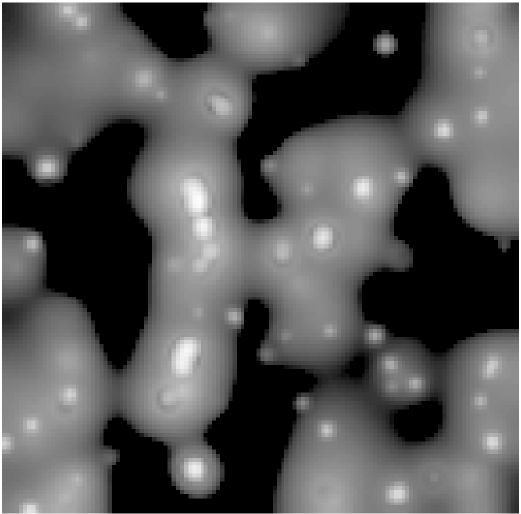
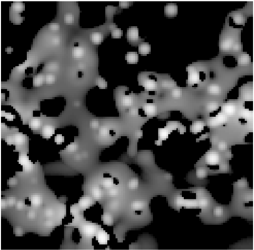
Figure 8: Wavelet denoising of a (model) galaxy distribution (left – a successful attempt, right – over-denoising)

The details of the algorithm we used are too tedious to describe in full, they can be found in Starck and Murtagh (ESstarck06 ).. The main points are:

1. We used the à trous algorithm, not an orthogonal one. The reason for that is that we needed to discriminate between the positions of significant wavelet amplitudes (the multiresolution support) and non-significant amplitudes at the last stage, and when speaking of positions, orthogonal wavelet transforms cannot be used.

2. We hard thresholded the solution and iterated it, reconstructing and transforming again, to obtain a situation where the final significant wavelet coefficients would cover exactly the original multiresolution support.

3. Finally, we smooth the solution by imposing a smoothness constraint, requiring that the sum of the absolute values of wavelet amplitudes of a given order would be minimal, while keeping the corrected amplitudes themselves within a given tolerance ($\sigma_{j}/2$) of the original noisy ones. We consider here only the amplitudes in the multiresolution support; this point required using a translation invariant wavelet transform.

Fig. 9 compares the results of our 3-D wavelet denoising. We started with a 3-D galaxy distribution, applied our algorithm to it, and, for comparison, built two Gaussian-smoothed density distributions. It is clearly seen that the typical details, in the case of Gaussian smoothing, are of uniform size, while the wavelet-denoised density distribution is adaptive, showing details of different scales.

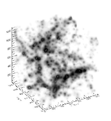
Figure 9: Density fields for a model galaxy distribution. Left – Gaussian $\sigma=1$ Mpc/$h$ smoothing, middle – wavelet denoising, right – Gaussian $\sigma=3$ Mpc/$h$ smoothing

2.5 Multiscale Densities

We have made an implicit assumption during all this section, namely, that a true density field exists. Is that so certain? Our everyday experience tells us that it is. But look at the numbers that stand behind this experience: even one cubic centimetre of air has $6\times 10^{23}/22.4\times 10^{3}\approx 3\times 10^{19}$ particles. In our surveys, one gigantic cosmological ’cubic centimetre’ of 10 Mpc size contains about 10 galaxies. Can we speak about their true spatial density?

One answer is that we can, but there are regions where the density estimates are extremely uncertain; statistics can tell us what the expected variances are. Another answer is that even if there is a true density, it is not always a useful physical quantity, especially for the largest scales we study. One of the reasons we measure the cosmological density field is to find its state of evolution and traces of initial conditions in it. The theory of the dynamics of perturbations in an expanding universe predicts that structure evolves at different rates, slowly at large scales and much more rapidly at galactic scales. Observations show that cosmological fields are multiscale objects; the recently determined power spectra span scales from about 600 Mpc/$h$ ($k=0.01\,h/\mathrm{Mpc}$ to 10 Mpc/$h$ ($k=0.6\,h/\mathrm{Mpc}$. Thus, should not these fields be studied in multiscale fashion, scale by scale? A true adaptive density mixes effects from different scales and scale separation could give us a cleaner look at the dynamics of large-scale structure.

In case of our everyday densities, this separation of scales can be done safely later, analyzing the true density. For galaxy distributions, it is wiser to prescribe a scale (range) and to obtain that density directly from the observed galaxy positions. One advantage is in accuracy, another in that there are places (voids), where, e.g., small-scale densities simply do not exist.

And this is the point where the first part of the lecture (wavelets) connects with the second part (density fields). The representation of the observed density fields by a sum of the densities of different characteristic scales (7) is just what we are looking for. True, there is a pretty large frequency overlap between the neighbouring bands (Fig. 10 shows you their power spectra), but that is possibly the best we can do, while keeping translational invariance. The figure shows also the power spectra of Gaussians of the same scales that are sometimes used to select different scales. As we see, Gaussian frequency bands are heavily correlated, the overlap of the smaller frequency band with that of the higher one is total, and that is natural – smoothing destroys signals of high frequency, but it does not separate frequency bands. So Gaussians should not be used in this business, but, alas, they frequently are.

Figure 10: Power spectra for two neighbouring scales, the $B_{3}$-associated à trous bands (solid lines), and for Gaussian smoothing of the same scales /(dotted lines). Only the positive half on the frequency axis is shown

Figs. 11 and 12 show the à trous density slices for a Gaussian cube. This is a $256^{3}$ realization of a Gaussian random field with a power spectrum approximating that of our universe. In real universe, the size of the cube would be 256 Mpc/$h$. The slices are taken from the same height; The images are in gray coding, black shows the densest regions. As in Fig. 7, the scaling solutions form the left column and the wavelets – the right column; transform orders grow downwards. In height, the wavelet orders are placed between the scaling order that produced them. The scaling solution of order three is repeated in Fig. 12 to keep the scaling–wavelet alignment. Enjoy.

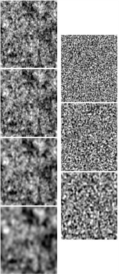
Figure 11: Á trous density (slices) of a Gaussian density field. (linear scale). The first orders (0–3 for the scaling solutions, 1–3 for the wavelets)

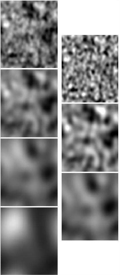
Figure 12: Á trous density (slices) of a Gaussian density field. (linear scale). The large-scale orders (3–6 for the scaling solutions, 4–6 for the wavelets)

3 Minkowski Functionals

Peter Coles explains in his lecture why it is useful to study morphology of cosmological fields. In short, it is useful because it is sort of a perpendicular approach to the usual moment methods. Our present cosmological paradigm says that the initial perturbation field was a realization of a Gaussian random field. The most direct test of that would be to measure all $n$-point joint amplitude distributions, starting from the 1-point distribution. Well, we know that even this is not Gaussian, but we know why (gravitational dynamics of a positive density field inevitably skews this distribution), and we can model it. As cosmological densities are pretty uncertain, the more uncertain are their many-point joint distributions. So this direct check does not work, at least presently.

Another possibility to check for Gaussianity is to estimate higher order correlation functions and spectra. For Gaussian realizations, odd-order correlations and power spectra should be zero, and even-order moments should be directly expressible via the second-order moments, the usual two-point correlation function and the power spectrum. Their dynamical distortions can also be modelled, and this is an active area of research.

Morphological studies provide an independent check of Gaussianity. Morphology of (density) fields depends on all correlation functions at once, is scale-dependent, but local, and can also be predicted and its change caused by dynamical evolution can be modelled. This lecture is, finally, about measuring morphology of cosmological fields.

An elegant description of morphological characteristics of density fields is given by Minkowski functionals ESmecke94 . These functionals provide a complete family of morphological measures – all additive, motion invariant and conditionally continuous functionals defined for any hypersurface are linear combinations of its Minkowski functionals.

The Minkowski functionals (MF for short) describe the morphology of iso-density surfaces, and depend thus on the specific density level. Of course, when the original data are galaxy positions, the procedure chosen to calculate densities (smoothing) will also determine the result. The usual procedure used in this business is to calculate kernel densities with wide Gaussian kernels; the recipes say that the width of the kernel (standard deviation) should be either the mean distance between galaxies or their correlation length, whichever is larger. Although this produces nice smooth densities, the recipe is bad, it destroys the texture of the density distribution; I shall show it later.

We shall use wavelets to produce densities, and shall look first at the texture of a true (wavelet-denoised) density, and then at the scale-dependent multiscale texture of the galaxy density distribution. We could also start directly from galaxies themselves, as Minkowski functionals can be defined for a point process, decorating the points with spheres of the same radius, and studying the morphology of the resulting surface. This approach does not refer to a density and we do not use it here. Although it is beautiful, too, the basic model that it describes is a (constant-density) Poisson process; a theory for that case exists, and analytical expressions for Minkowski functionals are known. Alas, as the galaxy distribution is strongly correlated, this reference model does not help us much. The continuous density case has a reference model, too, and that is a Gaussian random field, so this is more useful.

For a $d$-dimensional space, one can find $d+1$ different Minkowski functionals. We shall concentrate on usual 3-D space; for that, the Minkowski functionals are defined as follows. Consider an excursion set $F_{\phi_{0}}$ of a field $\phi(\mathbf{x})$ in 3-D (the set of all points where density is larger than a given limit, $\phi(\mathbf{x}\geq\phi_{0}$)). Then, the first Minkowski functional (the volume functional) is the volume of this region (the excursion set):

$$V_{0}(\phi_{0})=\int_{F_{\phi_{0}}}d^{3}x\;.$$ (29)

The second MF is proportional to the surface area of the boundary $\delta F_{\phi}$ of the excursion set:

$$V_{1}(\phi_{0})=\frac{1}{6}\int_{\delta F_{\phi_{0}}}dS(\mathbf{x})\;,$$ (30)

(but not the area itself, notice the constant). The third MF is proportional to the integrated mean curvature of the boundary:

$$V_{2}(\phi_{0})=\frac{1}{6\pi}\int_{\delta F_{\phi_{0}}}\left(\frac{1}{R_{1}(\mathbf{x})}+\frac{1}{R_{2}(\mathbf{x})}\right)dS(\mathbf{x})\;,$$ (31)

where $R_{1}(\mathbf{x})$ and $R_{2}(\mathbf{x})$ are the principal curvatures of the boundary. The fourth Minkowski functional is proportional to the integrated Gaussian curvature (the Euler characteristic) of the boundary:

$$V_{3}(\phi_{0})=\frac{1}{4\pi}\int_{\delta F_{\phi_{0}}}\frac{1}{R_{1}(\mathbf{x})R_{2}(\mathbf{x})}dS(\mathbf{x})\;.$$ (32)

The last MF is simply related to the genus that was the first morphological measure used in cosmology; all these papers bear titles containing the word ’topology’. Well, the topological Euler characteristic $\chi$ for a surface in 3D can be written as

$$\chi=\frac{1}{2\pi}\int_{S}\kappa\,dS\;,$$ (33)

where $\kappa$ is the Gaussian curvature, so

$$V_{3}=\frac{1}{2}\chi\;.$$ (34)

Bear in mind, though, that the Euler characteristic (33) describes the topology of a given iso-density surface, not of the full 3-D density distribution; the topology of the latter is, hopefully, trivial.

The first topology papers concentrated on the genus $G$ that is similar to $V_{3}$:

$$\chi=2(1-G)\;,\qquad V_{3}=1-G\;.$$ (35)

The functional $V_{3}$ is a bit more comfortable to use – it is additive, while $G$ is not, and in the case our surface breaks up into several isolated balls, $V_{3}$ is equal to the number of balls. If the excursion set contains only a few isolated empty regions (bubbles), $V_{3}$ gives their number. In a general case

$$V_{3}=\#\mbox{-of-balls}+\#\mbox{-of-bubbles}-\#\mbox{-of-tunnels}\;,$$

where only these tunnels that are open at both ends, count.

I have to warn you about a possible confusion with the genus relations (33–35) – the coefficient 2 (or 1/2) occupies frequently a wrong position. The confusion is due to a fact that two topological characteristics can be defined for an excursion set – one for its surface, another for the set itself. The relation between these depends on the dimensionality of the space; for 3-D the topological characteristic for the excursion set is half of that for the surface, and if we mix them up, our formulae become wrong. I know, we have published a wrong formula, too (even twice), but the formulae are right in our book ESmartsaar . So, bear in mind that the Minkowski functionals are calculated for surfaces, and use only the relations above (33–35). When in doubt, consult the classical paper by Mecke et al. ESmecke94 , and use the Crofton’s formula below (3.3) for a single cubic cell – it gives you $V_{3}=1\Rightarrow G=0$ .

Fig. 13 shows a Gaussian cube (a realization of a Gaussian random process) for two different smoothing widths (the left pair and the right pair of columns, respectively), and for three volume fractions. You can see that the solid figures inside the isodensity surface are awash with handles, especially at the middle 50% density level. Of course, the larger the smoothing, the less the number of handles. You can also see that Gaussian patterns are symmetric – the filled regions are exact lookalikes of the empty regions, for a symmetric change of volume fractions.

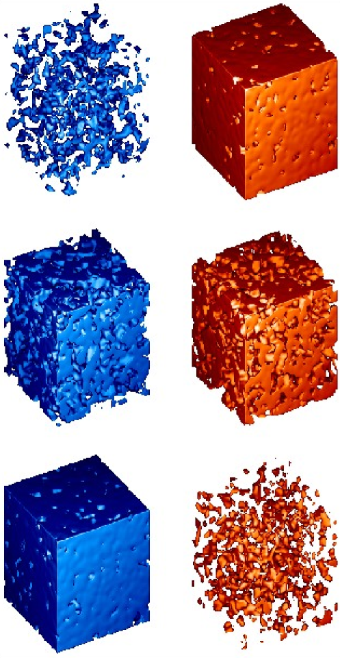
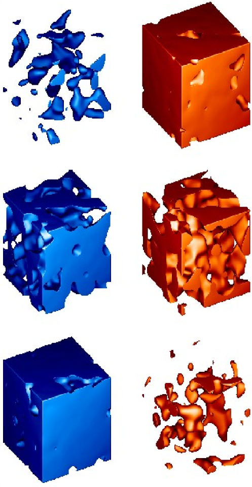
Figure 13: A Gaussian cube of $256^{3}$ pixels for different Gaussian smoothing filters. The left two columns show isodensity surfaces for $\sigma=3$ pixels, the right two columns – for $\sigma=8$ pixels. To better delineate isodensity surfaces, we show two sides of the surface in column pairs, where the left column shows high-density regions, and the right column – low-density regions for the same isodensity surface. The rows are for constant volume fractions (7%, 50%, and 93%), starting from below

Galaxy densities are more asymmetrical, as seen in Fig. 14. This figure shows a model galaxy distribution from a N-body simulation, in a smaller cube. The 50% density volumes differ, showing asymmetry in the density distribution, and the 5% – 95% symmetry, evident for the Gaussian cube, is not so perfect any more.

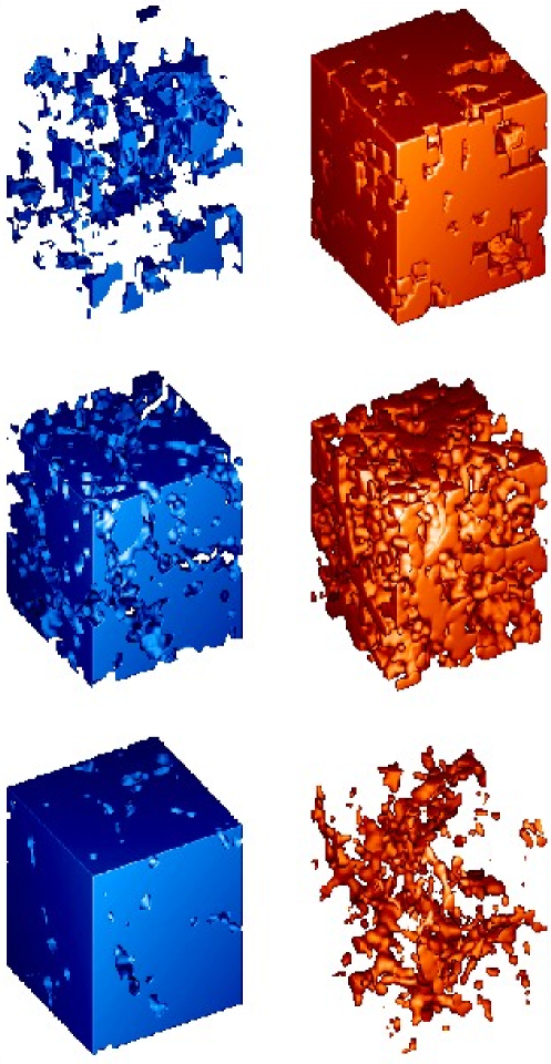
Figure 14: A galaxy sample ($60^{3}$ pixels) for a 3-pixel smoothing scale. The left column shows high-density regions, and the right column – low-density regions for the same isodensity surface. The rows are for constant volume fractions (7%, 50%, and 93%), starting from below

Instead of the functionals, their spatial densities $V_{i}$ are frequently used:

$$v_{i}(f)=V_{i}(f)/V\;,\quad i=0,\dots,3\;,$$

where $V$ is the total sample volume. The densities allow us to compare the morphology of different data samples.

3.1 Labelling the Isodensity Surfaces

The original argument of the functionals, the density level $\varrho_{0}$, can have different amplitudes for different fields, and the functionals are difficult to compare. Because of that, normalized arguments are usually used; the simplest one is the volume fraction $f_{v}$, the ratio of the volume outside of the excursion set to the total volume of the region where the density is defined (the higher the density level, the closer this ratio is to 1). Another, similar argument is the mass fraction $f_{m}$, which is very useful for real, positive density fields, but is cumbersome to apply for realizations of Gaussian fields, where the density may be negative. But when we describe the morphology of single objects (superclusters, say), the mass fraction is the most natural argument. It is also defined to approach 1 for the highest density levels (and for the smallest masses inside the isodensity surface).

The most widely used argument in this business is the Gaussianized volume fraction $\nu$, defined as

$$f_{v}=\frac{1}{\sqrt{2\pi}}\int_{\nu}^{\infty}\exp(-t^{2}/2)\,dt\;.$$ (36)

This argument was introduced already in the first topology paper by Gott ESgott86 , in order to eliminate the first trivial effect of gravitational clustering, the deviation of the 1-point pdf from the (supposedly) Gaussian initial pdf. Notice that using this argument, the first Minkowski functional is trivially Gaussian by definition.

Figure 15: The first two Minkowski functionals for N-body model galaxies. Here $v_{f}$ is the volume fraction, $m_{f}$ – the mass fraction, $\nu_{\sigma}$ – the normalized volume fraction, and $\nu_{G}\equiv\nu$ – the Gaussianized volume fraction from (36). The dotted line in the right panels shows the predicted Minkowski functionals for a Gaussian random field MF

For a Gaussian random field, $\nu$ is the density deviation from the mean, divided by the standard deviation. We can define a similar argument for any field:

$$\nu_{\sigma}=\frac{\varrho-\overline{\varrho}}{\sigma(\varrho)}\;.$$

I show different Minkowski functionals versus different arguments in Figs. 15 and 16. They are calculated for the model galaxy density distribution shown in the previous figure (Fig. 14). Note how much the shape of the same function(al)s depends on the arguments used.

Figure 16: The last two Minkowski functionals for N-body model galaxies. Here $v_{f}$ is the volume fraction, $m_{f}$ – the mass fraction, $\nu_{\sigma}$ – the normalized volume fraction, and $\nu_{G}\equiv\nu$ – the Gaussianized volume fraction from (36). The dotted line in the right panels shows the predicted Minkowski functionals for a Gaussian random field MF

3.2 Gaussian Densities

All the Minkowski functionals have analytic expressions for iso-density slices of realizations of Gaussian random fields. For three-dimensional space they are:

$$v_{0} = \frac{1}{2}-\frac{1}{2}\Phi\left(\frac{\nu}{\sqrt{2}}\right)\;,$$ (37)

$$v_{1} = \frac{2}{3}\frac{\lambda}{\sqrt{2\pi}}\exp\left(-\frac{\nu^{2}}{2}\right)\;,$$ (38)

$$v_{2} = \frac{2}{3}\frac{\lambda^{2}}{\sqrt{2\pi}}\nu\exp\left(-\frac{\nu^{2}}{2}\right)\;,$$ (39)

$$v_{3} = \frac{\lambda^{3}}{\sqrt{2\pi}}(\nu^{2}-1)\exp\left(-\frac{\nu^{2}}{2}\right)\;,$$ (40)

where $\Phi(\cdot)$ is the Gaussian error integral, and $\lambda$ is determined by the correlation function $\xi(r)$ of the field:

$$\lambda^{2}=\frac{1}{2\pi}\frac{\displaystyle\xi^{\prime\prime}(0)}{\displaystyle\xi(0)}\;.$$ (41)

The dimension of $\lambda$ is inverse length.

This expression allows to predict all the Minkowski functionals for a known correlation function (or power spectrum). We can also take a more empirical approach and to determine $\lambda^{2}$ on the basis of the observed density field itself, using the relations $\xi(0)=\langle\varrho^{2}\rangle$ and $\xi^{\prime\prime}(0)=\langle\varrho,_{i}^{2}\rangle$, where $\varrho,_{i}$ is the density derivative in one coordinate direction.

The expected form of these functionals is shown in Fig. 17.

Figure 17: Gaussian predictions for Minkowski functionals $\lambda=1$

In practice, it is easy to obtain good estimates of the Minkowski functionals for periodic fields. The real data, however, is always spatially limited, and the limiting surfaces cut the iso-density surface. An extremely valuable property of Minkowski functionals is that such cuts can be corrected for – the data volume mask is another body, and Minkowski functionals of intersecting bodies can be calculated. Moreover, if we can assume homogeneity and isotropy for the pattern, we can correct for border effects of large surveys. This is too technical for the lecture, so I refer to our forthcoming paper ESmfpaper2 .

3.3 Numerical Algorithms

Several algorithms are used to calculate the Minkowski functionals for a given density field and a given density threshold. We can either try to follow exactly the geometry of the iso-density surface, e.g., using triangulation, or to approximate the excursion set on a simple cubic grid. The first algorithms were designed to calculate the genus only; the algorithm that was proposed by Gott, Dickinson, and Melott ESgott86 uses a decomposition of the field into filled and empty cells, and another class of algorithms (Coles, Davies, and Pearson EScoles96 ) uses a grid-valued density distribution. The grid-based algorithms are simpler and faster, but are believed to be not as accurate as the triangulation codes.

I advocate a simple grid-based algorithm, based on integral geometry (Crofton’s intersection formula), proposed by Schmalzing and Buchert (ESjens ). It is similar to that of EScoles96 , and for $V_{3}$ (genus) coincides with it.

To start with, we find the density thresholds for given filling fractions $f$ by sorting the grid densities. This is a common step for all grid-based algorithms. Vertexes with higher densities than the threshold form the excursion set. This set is characterized by its basic sets of different dimensions – points (vertexes), edges formed by two neighbouring points, squares (faces) formed by four edges, and cubes formed by six faces. The algorithm counts the numbers of elements of all basic sets, and finds the values of the Minkowski functionals as

$$V_{0} = a^{3}N_{3}\;,$$

$$V_{1} = a^{2}\left(\frac{2}{9}N_{2}-\frac{2}{3}N_{3}\right)\;,$$

$$V_{2} = a\left(\frac{2}{9}N_{1}-\frac{4}{9}N_{2}+\frac{2}{3}N_{3}\right)\;,$$

$$V_{3} = N_{0}-N_{1}+N_{2}-N_{3}\;,$$ (42)

where $a$ is the grid step, $N_{0}$ is the number of vertexes, $N_{1}$ is the number of edges, $N_{2}$ is the number of squares (faces), and $N_{3}$ is the number of basic cubes in the excursion set.

This algorithm described above is simple to program, and is very fast, allowing the use of Monte-Carlo simulations for error estimation .

The first, and most used, algorithm was ’CONTOUR’ and its derivations; this algorithm was written by David Weinberg and was probably one of the first cosmological public-domain algorithms EScontour . However, there is a noticeable difference between the results that our grid algorithm produces and those of ’CONTOUR’. indexalgorithm:CONTOUR You can see it yourself, comparing the Minkowski functional figures in this lecture with Fig. 4 in Peter Coles’ chapter. All genus curves ever found by ’CONTOUR’ look like that there, very jaggy. How much I have tried, using Gaussian smoothing and changing smoothing lengths, I have never been able to reproduce these jaggies by our algorithm. At the same time, the calculated genus curves always follow the Gaussian prediction, so there is no bias in either algorithm. As the genus ($V_{3}$) counts objects (balls, holes, handles), it should, in principle, have mainly unit jumps, and only occasionally a larger jump. That is what we see in our genus ($V_{3}$) graphs. The only conclusion that I can derive is that the algorithm we use is more stable, with a much smaller variance.

3.4 Shapefinders

As Minkowski functionals give a complete morphological description of surfaces, it should be possible to use them to numerically describe the shapes of objects, right? For example, to differentiate between fat (spherical) objects and thin (cylindrical objects), banana-like superclusters and spiky superclusters. This hope has never died, and different shape descriptors have been proposed (a selection of them is listed in our book ESmartsaar ). The set of shape descriptors that use Minkowski functionals was proposed by Sahni, Sathyaprakash and Shandarin ESsahni , and is called ’shapefinders’. Now, shapefinder definitions have a habit of changing from paper to paper and it is not easy to follow the changes, so I shall give here a careful derivation of the last version of shapefinders. Shapefinders are defined as ratios of numbers that are similar to Minkowski functionals, but only close. in 3-D, the chain of Minkowski functionals $V_{i}$, from $V_{0}$ to $V_{3}$, has gradually diminishing dimensions, from $L^{3}$ to $L^{0}$. So, the ratios of neighbours in this chain have a dimension of length; these ratios make up the first set of shapefinders. The proportionality coefficients are chosen to normalize all these ratios to $R$ for a sphere of the radius $R$. Take a surface that is delimiting (shaping) a three-dimensional object (e.g., a supercluster). The definitions of the first three Minkowski functionals (29–31) can be rewritten as

$$V = V_{0}=\frac{4\pi}{3}R^{3}\;,$$

$$S = 6V_{1}=4\pi R^{2}\;,$$

$$C = 3\pi V_{2}=R\;,$$

where the second equalities stand for a sphere of a radius $R$, $V$ is the volume, $S$ – the surface, and $C$ – the mean integrated radius of curvature:

$$C=\int_{S}\frac{1}{2}\left(\frac{1}{R_{1}(\mathbf{x})}+\frac{1}{R_{2}(\mathbf{x})}\right)\,dS\;.$$ (43)

Whatever formulae you see in the literature, do not use them before checking with the definition below – these are the true shapefinders:

$$H_{1} = \frac{3V}{S}=\frac{1}{2}\frac{V_{0}}{V_{1}}\;,\quad\mathrm{thickness}\;,$$ (44)

$$H_{2} = \frac{S}{C}=\frac{2}{\pi}\frac{V_{1}}{V_{2}}\;,\quad\mathrm{breadth}\;,$$ (45)

$$H_{3} = \frac{C}{4\pi}=\frac{3}{4}V_{2}\;,\quad\mathrm{length}\;.$$ (46)

Only this normalization gives you $H_{i}=R$ for a sphere; check it. The descriptive names you see were given by the authors. There is a fourth shapefinder – the genus has been given the honour to stand for it, directly. As genus counts “minus” things (minus the number of isolated objects, minus the number of holes), the fourth Minkowski functional $V_{3}$ should be a better candidate.

The first set of shapefinders is accompanied by the ’second order’ shapefinders

$$K_{1} = \frac{H_{2}-H_{1}}{H_{2}+H_{1}}\;,\quad\mathrm{planarity}\;,$$ (48)

$$K_{2} = \frac{H_{2}-H_{1}}{H_{2}+H_{1}}\;,\quad\mathrm{filamentarity}\;.$$ (49)

These five (six, if you count the genus) numbers describe pretty well the shape of smooth (ellipsoidal) surfaces. In this case, the ratios $K_{1}$ and $K_{2}$ vary nicely from 0 to 1, and another frequently used ratio, $K_{1}/K_{2}$, has definite trends with respect to the shape of the object. But things get much more interesting when you start calculating the shapefinders of real superclusters; as shapes get complex, simple meanings disappear. Also, as shapefinders are defined as ratios of observationally estimated numbers (or ratios of quadratic combinations, as $H_{i}$ work out in terms of $V_{i}$), they are extremely noisy. So, in case of serious use, a procedure should be developed to estimate the shapefinders directly, not by the ratio rules (44, 48); such a procedure does not exist yet. But, for the moment, the shapefinders are probably the best shape description tool (for cosmology) we have.

3.5 Morphology of Wavelet-Denoised Density

So much for the preliminaries. Now we have all our tools (wavelets, densities, Minkowski functionals). Let us use them and see what is the morphology of the real galaxy density distribution.

This question has been asked and answered about a hundred times, starting from the first topology paper by Gott et al ESgott86 . The first data set was a cube from the CfA I sample and contained 123 galaxies, if I remember right. (Imagine estimating a spatial density on the basis of a hundred points; this is the moment that Landau’s definition of a cosmologist is appropriate: “Cosmologists are often wrong, but never in doubt”.) The answer was – Gaussian ! ; ten points for courage. The same optimistic answer has been heard about a hundred times since (in all the papers published), with slight corrections in later times, as data is getting better. These corrections have been explained by different observational and dynamical effects, and peace reigns.

But – all these studies have carefully smoothed the galaxy catalogues by nice wide Gaussian kernels to get a proper density. Doubts have been expressed that one Gaussianity could lead to another (by Peter Coles, for example), and the nice Gaussian behaviour we get is exactly that we have built in in the density field. So, let us wavelet-denoise the density field (a complex recipe, but without any Gaussians), and estimate the Minkowski functionals. The next two figures are from our recent work (ESmfpaper1 ).

The data are the 2dFGRS Northern galaxies; we chose a maximum-volume one-magnitude interval volume-limited (constant density) sample and cut a maximum-volume brick from it (interesting, every time I say ’maximum’, the sample gets smaller). Constant density is necessary, otherwise typical density scales will change with distance, and a brick was cut in order to avoid border corrections (these can bring additional difficulties for wavelet denoising). We carefully wavelet-denoised the density; Fig. 18 shows its fourth Minkowski functional.

Figure 18: The Minkowski functional $V_{3}$ for the 2dF brick, for the wavelet denoised data set (thick solid line). The variability range of the wavelet denoised mocks is shown with bars. We show also the 95% confidence limits for 1300 realizations of theoretical Gaussian density fields (dashed lines), and the $V_{3}$ data curve (thin solid line), all obtained for the Gaussian $\sigma=2$ Mpc/$h$ smoothing

First, we see that our wavelet.denoised density is never close to Gaussian. Secondly, the specially built N-body catalogues (mocks) do not have Gaussian morphology, too; although they deviate from the real data, they are closer to it than to the example Gaussian. We see also that the same galaxies, smoothed by a yet very narrow Gaussian kernel ($\sigma=2$ Mpc/$h$), show an almost Gaussian morphology. Thus, the clear message of this figure is that the morphology of a good (we hope the best) adaptive galaxy density is far from Gaussian; and the Gaussianity-confirming results obtained so far are all the consequence of the Gaussianity input by hand – Gaussian smoothing. This figure exhibits a little non-Gaussianity yet; the next one (Fig. 19) almost does not. The filter used there is still narrow ($\sigma=4$ Mpc/$h$); the filter widths used in most papers are around twice that value.

Figure 19: The Minkowski functional $V_{3}$ for the 2dF brick, Gaussian smoothed with $\sigma=4$ Mpc/$h$ (thick solid line). The variability range of the mocks is shown with bars. We show also the 95% confidence limits for 1300 realizations of theoretical Gaussian density fields (dashed lines).

I am pretty sure that Gaussian smoothing is the culprit here. We built completely non-Gaussian density distributions (Voronoi walls and networks), Gaussian smoothed them using popular recipes about the kernel size, and obtained perfectly Gaussian Minkowski functionals.

One reason for that, as Vicent Martínez has proposed, is that the severe smoothing used changes a density field into Poissonian, practically. Try it – smooth a density field with a Gaussian of $\sigma=r_{0}$, where $r_{0}$ is the correlation length, and you get a density field with a very flat low-amplitude correlation function, almost Poissonian. And the Minkowski functionals of Poissonian density fields are Gaussian; we tested that.

Another reason that turns Minkowski functionals Gaussian even for small $\sigma$, must be the extended wings of Gaussian kernels. Although they drop pretty fast, they are big enough to add to a small extra ripple on the main density field. As Minkowski functionals are extremely sensitive to small density variations, then all they see is that ripple. This is especially well seen in initially empty regions. Usually, one uses a FFT-based procedure for Gaussian smoothing, as that is at least a hundred times faster (for present catalogue volumes) that direct convolution in real space. This procedure generates a wildly fluctuating small-amplitude density field in empty regions, and we did not realize for a long time at first where those giant-amplitude ghost MF-s came from. Gaussian smoothing and FFT, that was their address.

3.6 Multiscale Morphology

So, the galaxy density, similar to that we have accustomed to find in our everyday experience, is decidedly non-Gaussian. But is that a problem? Cosmological dynamics tells us that structure evolves at different rate at different scales; a true density mixes these scales all together and is not the best object to search for elusive traces of initial conditions. Good. Multiscale densities to the rescue.

The results that will end this chapter did not exist at the time of the summer school. But we live in the present, and time is short, so I will include them. A detailed account is already accepted for publication (ESmfpaper2 ), I shall show only a collection of Minkowski functionals here.

As our basic data set, we took the 2dFGRS volume-limited samples for the $[-20,-19]$ magnitude interval; they have the highest mean density among similar one-magnitude interval samples. We did not cut bricks this time, but corrected for sample boundaries; we have learnt that by now. We wavelet-decomposed the galaxy density fields and found the Minkowski functionals; as simple as that. Although wavelet decompositions are linear and should not add anything to the morphology of the fields, we checked that on simulated Gaussian density fields. Right, they do not add any extra morphological signal.

The results (for the 2dFGRS North) are shown in Figs. 20–22. As the amplitudes of the (densities of) Minkowski functionals vary in a large interval, we use a sign-aware logarithmic mapping:

$$\mathrm{logn}(x;a)=\mathrm{sgn}(x)\log(1+|x|/a)\;.$$

This mapping accepts arguments of both signs ($\log(x)$ does not), is linear for $|x|<<a$ and logarithmic for $|x|>>a$. As the figures show, for the scales possible to study, the morphology of the galaxy density distribution is decidedly not Gaussian. The deviations are not too large for the second Minkowski functional $v_{2}$ (watch how the maxima shift around), but are clearly seen for the two others. The maximum wavelet order here is 3 for a $\sqrt{2}$ Mpc/$h$ grid, that corresponds to a characteristic scale of $2^{3}\sqrt{2}\approx 11.3$ Mpc/$h$. As the mean thickness of the 2dFGR North slice is about 40–50 Mpc/$h$, we cannot go much further – the higher order wavelet slices would be practically two-dimensional. The 2dFGRS Southern dataset has similar size limitations. So, as 10 Mpc/$h$ is a scale where cosmological dynamics might have slight morphological effects, the question if the original morphology of the cosmological density field was Gaussian, is not answered yet. But we shall find it out soon, when the SDSS will finally fill its full planned volume.

Figure 20: Summary of the densities of the second MF $v_{1}$ for the data and all wavelet orders for the 2dFN19 sample, in the logn mapping. Thick lines show reference Gaussian predictions. Full lines stand for the 1 Mpc/$h$ grid, dotted lines – for the $\sqrt{2}$ Mpc/$h$ grid

Figure 21: Summary of the densities of the third MF $v_{2}$ for the data and all wavelet orders for the 2dFN19 sample, in the logn mapping. Thick lines show reference Gaussian predictions. Full lines stand for the 1 Mpc/$h$ grid, dotted lines – for the $\sqrt{2}$ Mpc/$h$ grid

Figure 22: Summary of the densities of the fourth MF $v_{3}$ for the data and all wavelet orders for the 2dFN19 sample, in the logn mapping. Thick lines show reference Gaussian predictions. Full lines stand for the 1 Mpc/$h$ grid, dotted lines – for the $\sqrt{2}$ Mpc/$h$ grid

These are the results, for the moment. The morphology of the galaxy density field is far from Gaussian, in contrary to practically every earlier result. Have all these results only confirmed that if we take a serious smoothing effort, we are able to smooth any density field to Poissonian? An indecent thought.

But do not be worried, results come and go, this is the nature of research. Methods, on the contrary, stay a little longer, and this school was all about methods.

Recommended Reading

I was surprised that Bernard Jones recommended a wavelet bookshelf that is almost completely different from mine (the only common book is that of I. Daubechies’). So, read those of Bernard’s choice, and add mine:

• five books:

  1. Stephane Mallat, A Wavelet Tour of Signal Processing, 2nd ed., Academic Press, London, 1999,

  2. C. Sidney Burrus, Ramesh A. Gopinath, Haitao Gao, Introduction to Wavelets and Wavelet Transforms, Prentice Hall, NJ, 1997,

  3. Ingrid Daubechies, Ten lectures on wavelets, SIAM, Philadelphia, 2002,

  4. Jean-Luc Starck, Fionn Murtagh, “Astronomical Image and Data Analysis”, 2nd ed., Springer, 2006 (application of wavelets and many other wonderful image processing methods in astronomy),

  5. Bernard W. Silverman, Density Estimation for Statistics and Data Analysis, Chapman & Hall / CRC Press, Boca Raton, 1986 (the classical text on density estimation),

• three articles:

  1. Mark J. Shensa, The Discrete wavelet Transform: Wedding the À Trous and Mallat Algorithms, IEEE Transactions on Signal Processing, 40, 2464–2482, 1992 (the title explains it all),

  2. K.R. Mecke, T. Buchert, H. Wagner, Robust morphological measures for large-scale structure in the Universe, Astron. Astrophys. 288, 697–704, 1994 (introducing Minkowski functionals in cosmology),

  3. Jens Schmalzing, Thomas Buchert, Beyond Genus Statistics: A Unified Approach to the Morphology of Cosmic Structure, Ap. J. Letts 482, L1, 1997, (presentation of two grid algorithms).

• two web pages:

  1. a wavelet tutorial by Jean-Luc Starck at (http://jstarck.free.fr),

  2. the wavelet pages by David Donoho at http://www-stat.stanford.edu/~donoho/ (look at lectures and reports).

References

- (1) Y. Ascasibar, J. Binney, MNRAS 356, 872–882, 2005
- (2) C. de Boor, A Practical Guide to Splines. Springer-Verlag, New York, 1978
- (3) P. Coles, A.G. Davies, R.C. Pearson, MNRAS 281, 1375, 1996
- (4) J.R. Gott, M. Dickinson, A.L. Melott, ApJ. 306, 341 1986
- (5) M. Holtschneider, R. Kronland-Martinet, J. Morlet, P. Tchamitchian. In: Wavelets, Time-Frequency Methods and Phase Space, Springer-Verlag, Berlin, 289–297, 1989
- (6) V.J. Martínez, E. Saar, Statistics of the Galaxy Distribution, Chapman & Hall /CRC Press, Boca Raton, 2002
- (7) V.J. Martínez, J.-L. Starck, E. Saar, D.L. Donoho, S.C. Reynolds, P. de la Cruz, S. Paredes, ApJ. 634, 744
- (8) K.R. Mecke, T. Buchert, H. Wagner, A&A 288, 697–704, 1994
- (9) W.H. Press, B.P. Flannery, S.A. Teukolsky, W.T. Vetterling, Numerical Recipes in C: The Art of Scientific Computing, CUP, Cambridge, 1992
- (10) E. Saar, V.J. Martínez, J.-L. Starck, D. Donoho, MNRAS (accepted), astro-ph/0610958, 2006
- (11) V. Sahni, B.S. Sathyaprakash, S.F. Shandarin, ApJ. Lett. 495, L5–L8, 1998
- (12) J. Schmalzing, T. Buchert, ApJ. Lett. 482, L1, 1997
- (13) B.W. Silverman, Density Estimation for Statistics and Data Analysis, Chapman & Hall / CRC Press, Boca Raton, 1986
- (14) J.-L. Starck, F. Murtagh, Astronomical Image and Data Analysis, 2nd ed., Springer, NY, 2006
- (15) D.H. Weinberg, PASP 100, 1373–1385, 1988