Physical Properties, Baryon Content, and Evolution of the Ly$\alpha$ Forest: New Insights from High Resolution Observations at $z\lesssim 0.4$

Abstract

We present a study of the Ly$\alpha$ forest at $z\lesssim 0.4$ from which we conclude that at least 20% of the total baryons in the universe are located in the highly-ionized gas traced by broad Ly$\alpha$ absorbers. The cool photoionized low-$z$ intergalactic medium (IGM) probed by narrow Ly$\alpha$ absorbers contains about 30% of the baryons. We further find that the ratio of broad to narrow Ly$\alpha$ absorbers is higher at $z\lesssim 0.4$ than at $1.5\lesssim z\lesssim 3.6$, implying that a larger fraction of the low redshift universe is hotter and/or more kinematically disturbed. We base these conclusions on an analysis of 7 QSOs observed with both FUSE and the HST/STIS E140M ultraviolet echelle spectrograph. Our sample has 341 H I absorbers with a total unblocked redshift path of 2.064. The observed absorber population is complete for $\log N_{\rm HI}\gtrsim 13.2$, with a column density distribution $f(N_{\rm HI})\propto N^{-\beta}_{\rm HI}$. For narrow ($b\leq 40$ ${\rm km\,s}^{-1}$) absorbers $\beta=1.76\pm 0.06$. The distribution of the Doppler parameter $b$ at low redshift implies two populations: narrow ($b\leq 40$ ${\rm km\,s}^{-1}$) and broad ($b>40$ ${\rm km\,s}^{-1}$) Ly$\alpha$ absorbers (referred to as NLAs and BLAs, respectively). Both the NLAs and some BLAs probe the cool ($T\sim 10^{4}$ K) photoionized IGM. The BLAs also probe the highly-ionized gas of the warm-hot IGM ($T\simeq 10^{5}$–$10^{6}$ K). The distribution of $b$ has a more prominent high velocity tail at $z\lesssim 0.4$ than at $1.5\lesssim z\lesssim 3.6$, which results in median and mean $b$-values that are 15–30% higher at low $z$ than at high $z$. The ratio of the number density of BLAs to NLAs at $z\lesssim 0.4$ is a factor of $\sim$3 higher than at $1.5\lesssim z\lesssim 3.6$.

1. Introduction

Observations of Ly$\alpha$ absorption lines in the spectra of QSOs provide a sensitive probe of the evolution and the distribution of the gas in the universe from high to low redshift. A forest of H I absorption lines occurs at different redshifts, $z$, along QSO sightlines with $\log N_{\rm HI}<17$. Understanding the evolution of the Ly$\alpha$ forest with redshift is critical to understanding the evolution and formation of structures in the universe. At $z\gtrsim 1.5$, observations of the Ly$\alpha$ forest are obtained from ground-based telescopes at a spectral resolution of 7–8 ${\rm km\,s}^{-1}$ using 8–10 m class telescopes (e.g., Hu et al., 1995; Lu et al., 1996; Kirkman & Tytler, 1997; Kim et al., 1997, 2002a), but at $z\leq 1.5$ they require UV space-based instruments. Space-based UV astronomy has produced remarkable results, including the discovery itself of the Ly$\alpha$ forest at low redshift (Bahcall et al., 1991; Morris et al., 1991). However, most of the UV studies of the IGM at low $z$ have lacked the spectral resolution and wavelength coverage of the higher redshift studies (Weymann et al., 1998; Impey et al., 1999; Penton et al., 2000, 2004), requiring assumptions for the Doppler parameter to derive the column density. The situation at $z\lesssim 0.5$ has dramatically improved in the last few years with high quality observations of several low redshift QSOs obtained with the Hubble Space Telescope (HST) and its Space Telescope Imaging Spectrograph (STIS). In its E140M echelle mode, STIS provides a spectral resolution of $\sim$7 ${\rm km\,s}^{-1}$, comparable to the resolution of the high redshift observations of the Ly$\alpha$ forest. The high spectral resolution has allowed the derivation of accurate Doppler parameters, $b$, and column densities, $N$, using techniques similar to those used at high redshift. The Doppler parameter is important because it is related to the temperature of the gas via $b^{2}=b^{2}_{\rm th}+b^{2}_{\rm nt}$, where $b_{\rm nt}$ is the non-thermal broadening of the absorption line and $b_{\rm th}=\sqrt{2kT/m}=0.129\sqrt{T}$ is the thermal broadening of the H I absorption line; therefore the measured $b$ directly provides an upper limit to the temperature of the observed gas.

In parallel, hydrodynamic cosmological simulations of the local universe have quickly evolved in recent years (Davé et al., 1999; Cen & Ostriker, 1999; Davé et al., 2001; Cen & Fang, 2006; Cen & Ostriker, 2006). These models predict that at low redshift roughly 30–50% of the baryons are in a hot (10⁵–10⁷ K) and highly ionized intergalactic medium (IGM) known as the warm-hot intergalactic medium (WHIM), 30–40% are in a cooler medium ($\lesssim 10^{4}$ K) photoionized by the UV background, and the remaining baryons are in galaxies. Observationally, Penton et al. (2004) found with moderate spectral resolution (FWHM $\sim$20 ${\rm km\,s}^{-1}$) UV observations that the cool phase of the IGM may contain 29% of the baryon budget. The observational detection of the WHIM came first from an intensive search of collisionally-ionized O VI systems and other highly ionized species such as Ne VIII using space-based observatories such as the Far Ultraviolet Spectroscopic Explorer (FUSE) and HST/STIS (e.g., Tripp, Savage, & Jenkins, 2000; Danforth & Shull, 2005; Savage et al., 2005). The baryon content of the O VI absorbers suggests that $\Omega_{\rm b}($O VI$)\gtrsim 0.0022h_{70}^{-1}$ or at least 5% of the total baryon budget (Sembach et al., 2004; Tripp et al., 2006; Danforth & Shull, 2005), but this estimate relies critically on the assumed oxygen abundance and the number of collisionally ionized O VI systems versus photoionized O VI systems (Prochaska et al., 2004; Lehner et al., 2006). The O VI systems probe the lower end of the WHIM temperature range ($T<10^{6}$ K). Higher temperatures can be traced with more highly ionized oxygen ions (O VII, O VIII) that can be observed in principle with X-ray observatories such as Chandra (Nicastro et al., 2005; Fang et al., 2006) and XMM-Newton, but the IGM detections of O VII and O VIII are still controversial (Kaastra et al., 2006; Rasmussen et al., 2006) for $z>0$.

The WHIM can also be detected through broad H I absorption lines. The high temperature of the WHIM will broaden the Ly$\alpha$ absorption line resulting in a large Doppler parameter ($b>40$ ${\rm km\,s}^{-1}$). A very small fraction of H I (typically $<10^{-5}$) is expected to be found in the highly ionized plasma of the WHIM, so that the broader the H I absorption line is, the shallower it should be. Recent observations, both with moderate spectral resolution and with the higher-resolution STIS E140M echelle mode, have revealed the presence of broad H I absorption lines that could be modeled by smooth and broad Gaussian components (Tripp et al., 2001; Bowen et al., 2002; Richter et al., 2004; Sembach et al., 2004; Lehner et al., 2006). H I absorbers with $b<40$ ${\rm km\,s}^{-1}$ imply that the temperature of these absorbers must be $T<10^{5}$ K. Since the nominal lower temperature of the WHIM is $T\sim 10^{5}$ K, it is a priori natural to consider two different physical populations of H I absorbers: the narrow Ly$\alpha$ absorbers (NLAs) as H I systems having $b<40$ ${\rm km\,s}^{-1}$ and the broad Ly$\alpha$ absorbers (BLAs) as H I systems having $b\geq 40$ ${\rm km\,s}^{-1}$. We will see that the separation between the NLAs and BLAs is not so evident observationally, with an important overlap between the two populations, particularly in the range $b=40$–50 ${\rm km\,s}^{-1}$. While it is clear that the NLAs are tracing mostly the cool photoionized IGM, the situation is less clear for the BLAs. There is a fuzziness in the separation of the BLAs from the NLAs because non-thermal broadening can be important and unresolved components can hide the true structure of the H I absorbers. Recent simulations show that non-thermal broadening could be particularly important for the H I absorbers with $40\lesssim b\lesssim 60$ ${\rm km\,s}^{-1}$ (Richter et al., 2006a). Therefore BLAs may probe photoionized gas (that can be either cool ($T\lesssim 10^{4}$ K) or hot ($T\gtrsim 10^{5}$ K) but with a very low density ($\log n_{\rm H}<-5.3$)) and  collisionally ionized, hot ($T\gtrsim 10^{5}$ K) gas. In this paper, we define a BLA as an absorber that can be fitted with a single Gaussian component with $b>40$ ${\rm km\,s}^{-1}$ (a NLA has $b\leq 40$ ${\rm km\,s}^{-1}$ and can have multiple components). BLAs probe the IGM that is either hotter ($b_{\rm th}\gg b_{\rm nt}$) or is more kinematically disturbed ($b_{\rm nt}\gg b_{\rm th}$) than the IGM probed by the NLAs. Studying in detail the NLA and BLA populations is also important for estimating the baryon density because an accurate inventory of the baryon distribution must separate the fraction of the baryons that are located in the cool photoionized IGM versus those that are in the substantially hotter shock-heated WHIM phase. The narrow and broad Ly$\alpha$ lines provide a means to discriminate between the cool and shock-heated gas clouds. Therefore to make a reliable assessment of the baryonic content of the Ly$\alpha$ forest at low z, it is necessary to investigate the frequency and properties of the NLAs and BLAs. The current estimate of the baryon budget residing in the BLAs over a redshift path $\Delta z=0.928$ yields $\Omega_{\rm b}({\rm BLA})\gtrsim 0.0027h_{70}^{-1}$ or at least 6% of the total baryon budget (Richter et al., 2006b), assuming that the observed broadening is mostly thermal and collisional ionization equilibrium applies.

In this paper, we will address these issues using a sample of 7 QSO sightlines that have been observed with both STIS E140M and FUSE and for which the data have been fully analyzed using similar techniques and are in press or to be submitted soon. While the spectral resolution of FUSE is only $\sim$20 ${\rm km\,s}^{-1}$ compared to $\sim$7 ${\rm km\,s}^{-1}$ for STIS E140M, FUSE gives access to several Lyman series and metal lines making the line identification more reliable and providing an unprecedented insight of the physical conditions and metallicity. The fundamental parameters of the Ly$\alpha$ forest lines (redshift $z$, column density $N$, and Doppler parameter $b$) were accurately determined using profile fitting of all the observed Lyman series lines. Because $b$ could be derived, this is the first time with a large sample that the properties of the Ly$\alpha$ forest in the low redshift universe can be studied as a function of $b$. The main aims of this work are 1) to study the distribution and evolution of the Doppler parameter of the Ly$\alpha$ forest, and 2) to determine the baryon density of the Ly$\alpha$ forest in the NLA and BLA populations. The organization of this paper is as follows: §2 describes the sample and its completeness; in §3 we study the distribution of the Doppler parameter $b$ and the Ly$\alpha$ density number as a function of $b$; in §4 we study the evolution of $b$ with redshift by comparing the low-$z$ ($z\lesssim 0.4$) Ly$\alpha$ forest with the mid-$z$ ($0.5\lesssim z\lesssim 1.5$) and high-$z$ ($1.5\lesssim z\lesssim 3.6$) Ly$\alpha$ forest; in §5 we estimate the column density distribution; and finally, in §6 we estimate the baryon content of the cool photoionized IGM probed by the NLAs and the photoionized IGM and the WHIM probed by the BLAs, and discuss the uncertainties in estimating the baryon budget. We summarize our results in §7.

Table 1Line of Sight Properties

Sightline	S/N	$z$	$\Delta z$	$\Delta X$	Refs.
(1)	(2)	(3)	(4)	(5)	(6)
H 1821+643	15–20	0.297	0.238	0.266	(1)
HE 0226–4110	5–11	0.495	0.401	0.481	(2)
HS 0624+6907	8–12	0.370	0.329	0.383	(3)
PG 0953+415	7–11	0.239	0.202	0.222	(4)
PG 1116+215	10–15	0.176	0.126	0.134	(5)
PG 1259+593	9–17	0.478	0.355	0.418	(6)
PKS 0405–123	5–10	0.574	0.413	0.498	(7)

Note. — Column 2: Range of signal-to-noise (S/N) per resolution element in STIS E140M mode. Column 3: QSO redshift. Column 4: Unblocked redshift path for Ly$\alpha$. Column 5: Absorption distance (see §2). Column 6: References: (1) Sembach et al. (2007, in prep.), (2) Lehner et al. (2006), (3) Aracil et al. (2006), (4) T.M. Tripp (2006, priv. comm.), (5) Sembach et al. (2004), (6) Richter et al. (2004), (7) Williger et al. (2006) and appendix of this paper.

2. The Low $z$ Sample

2.1. Description of the Sample and Completeness

Our low-$z$ sample consists of 7 QSO sightlines that were observed with HST/STIS E140M and FUSE: H 1821+643 (Sembach et al. 2007, in preparation; see also Tripp, Savage, & Jenkins 2000 and Oegerle et al. 2000 for the metal-line systems), HE 0226–4110 (Lehner et al., 2006), HS 0624+6907 (Aracil et al., 2006a), PG 0953+415 (T.M. Tripp 2006, private communication; see also Savage et al. 2002 for the metal-line systems), PG 1259+593 (Richter et al., 2004), PG 1116+215 (Sembach et al., 2004), and PKS 0405–123 (Williger et al. 2006; see also Prochaska et al. 2004 for the metal-line systems). Note that for HS 0624+6907, we used the results summarized in the erratum produced by Aracil et al. (2006b). The data handling and analysis are described in detail in the above papers. For PKS 0405–123, we adopt the new measurements and a new line list that we describe in the Appendix. The motivation to revisit Williger et al.’s analysis was first driven by differentiating a real detection from a noise feature for the BLAs since these authors noted that several of their BLAs could be just noise. This re-analysis also provides an overall coherent data sample that was analyzed following the same methodology. Signal-to-noise (S/N) where Ly$\alpha$ can be observed, redshift ($z$), unblocked redshift path ($\Delta z$), and absorption distance ($\Delta X$) are summarized in Table 1 for each sightline. The absorption distance was computed assuming a Friedman cosmology, $\Delta X=0.5[(1+\Delta z)^{2}-1]$ with $q_{0}=0$. For the lines of sight to QSOs with $z_{\rm QSO}<0.42$, we have excluded absorption systems within 5000 ${\rm km\,s}^{-1}$ of the QSO redshift. Some observations of low-redshift QSOs have provided evidence that “intrinsic” absorption lines can arise in clouds that are spatially close to the QSO and yet, due to the cloud kinematics, are substantially offset in redshift from the QSO (e.g., Yuan et al. 2002; Ganguly et al. 2003). To avoid contaminating the sample with these intrinsic absorbers, we do not use systems detected with 5000 ${\rm km\,s}^{-1}$ of the QSO. The Voigt profile fitting method was employed for each line of sight to measure the column densities ($N_{\rm HI}$), Doppler parameters ($b$), and redshifts of the absorbers and we adopt those results for our analysis. Table 2 lists these parameters. For PG 1259+593 we did not include in our sample the systems marked uncertain (UC) in Table 5 of Richter et al. (2004). A colon in Table 2 indicates that there is uncertainty in the determination of the physical parameters, which are not accounted for in the formal errors produced by the profile fitting. These systems are not taken into account when we use an error cutoff (see below). If we had, it would not have changed the results presented in this paper in a statistically significant manner.

The total sample consists of 341 H I systems, with a total unblocked redshift path $\Sigma\Delta z=2.064$ and a total absorption distance $\Sigma\Delta X=2.404$. There are 201 systems at $z\leq 0.2$ and 131 systems at $0.2<z\leq 0.4$. The remaining 9 systems lie at $0.4<z<0.44$. Therefore, our sample mostly probes the universe at $z\leq 0.4$. More absorbers are found at $z<0.2$ because several lines of sight do not extend out to $z=0.3$–0.4 and to a lesser extent because the S/N at $\lambda>1650$ Å decreases rapidly (see below).

Table 2H I measurements

$z$	$\log N_{\rm HI}$	$b$
	(dex)	(${\rm km\,s}^{-1}$)
H 1821+643 (Sembach et al. 2006, in prep.)
0.02438	$14.28\,^{+0.06}_{-0.05}$	$26.9\pm 1.7$
0.02642	$13.26\,^{+0.07}_{-0.08}$	$48.6\pm 6.0$
0.06718	$13.72\,^{+0.01}_{-0.01}$	$20.2\pm 0.6$
0.07166	$13.87\,^{+0.02}_{-0.02}$	$34.0\pm 1.0$
0.08911	$13.01\,^{+0.06}_{-0.07}$	$23.3\pm 2.8$
0.11133	$12.95\,^{+0.10}_{-0.13}$	$88.0\pm 14.0$
0.11166	$12.99\,^{+0.08}_{-0.09}$	$28.6\pm 4.4$
0.11961	$13.15\,^{+0.05}_{-0.06}$	$36.8\pm 3.4$
0.12055	$12.64\,^{+0.13}_{-0.18}$	$22.5\pm 5.9$
0.12112	$13.93\pm 0.37$	$26.0\,^{+13.0}_{-9.0}$
0.12125	$14.04\pm 0.36$	$40.0\,^{+44.0}_{-21.0}$
0.12147	$13.78\pm 0.17$	$85.0\,^{+37.0}_{-26.0}$
0.12221	$13.19\,^{+0.06}_{-0.06}$	$41.7\pm 4.4$
0.14754	$13.51\,^{+0.03}_{-0.03}$	$44.6\pm 2.5$
0.14776	$13.30\,^{+0.04}_{-0.05}$	$19.2\pm 1.6$
0.15731	$13.11\,^{+0.05}_{-0.06}$	$22.9\pm 2.1$
0.16127	$12.74\,^{+0.10}_{-0.12}$	$21.5\pm 4.0$
0.16352	$13.17\,^{+0.06}_{-0.07}$	$52.2\pm 5.9$
0.16966	$13.93\,^{+0.02}_{-0.02}$	$35.7\pm 2.0$
0.17001	$13.65\,^{+0.02}_{-0.02}$	$\cdots$
0.17051	$13.40\,^{+0.04}_{-0.04}$	$21.1\pm 1.4$
0.17926	$12.87\,^{+0.09}_{-0.12}$	$18.4\pm 3.4$
0.18047	$13.14\,^{+0.07}_{-0.08}$	$50.7\pm 6.6$
0.19662	$12.98\,^{+0.07}_{-0.08}$	$21.1\pm 2.7$
0.19904	$12.74\,^{+0.12}_{-0.17}$	$22.1\pm 5.4$
0.20957	$13.10\,^{+0.03}_{-0.04}$	$16.2\pm 0.9$
0.21161	$13.16\,^{+0.06}_{-0.06}$	$22.3\pm 2.3$
0.21668	$12.88\,^{+0.08}_{-0.10}$	$19.7\pm 3.0$
0.21326	$14.41\,^{+0.04}_{-0.04}$	$43.0\pm 2.4$
0.22497	$15.53\,^{+0.05}_{-0.05}$	$25.0\pm 7.0$
0.22616	$13.51\,^{+0.04}_{-0.04}$	$54.7\pm 3.8$
0.22786	$13.26\,^{+0.03}_{-0.04}$	$35.3\pm 2.0$
0.23869	$12.86\,^{+0.10}_{-0.12}$	$20.2\pm 3.8$
0.24142	$13.12\,^{+0.03}_{-0.04}$	$23.4\pm 1.4$
0.24531	$13.06\,^{+0.08}_{-0.10}$	$34.2\pm 5.1$
0.25689	$12.80\,^{+0.11}_{-0.15}$	$22.6\pm 5.1$
0.25814	$13.38\,^{+0.10}_{-0.13}$	$60.3\pm 8.8$
0.25816	$12.98\,^{+0.11}_{-0.15}$	$14.5\pm 3.4$
0.26152	$13.70\,^{+0.02}_{-0.03}$	$37.7\pm 1.5$
0.26659	$13.64\,^{+0.03}_{-0.03}$	$44.5\pm 2.1$
HE 0226–4110 (Lehner et al., 2006)
0.01746	$13.22\pm 0.06$	$17.9\pm 4.3$
0.02679	$13.22\pm 0.08$	$41.6\pm 11.0$
0.04121	$12.82\pm 0.14$	$23.6\pm 18.6$
0.04535	$12.71\pm 0.13$	$16.2\pm 12.8$
0.04609	$13.66\pm 0.03$	$25.0\pm 2.1$
0.06015	$13.19\pm 0.06$	$35.5\pm 7.6$
0.06083	$14.65\pm 0.02$	$44.5\pm 1.0$
0.07023	$13.81\pm 0.11$	$26.0\pm 12.4$
0.08375	$13.67\pm 0.05$	$29.6\pm 4.5$
0.08901	$13.33\pm 0.05$	$23.8\pm 3.7$
0.08938	$12.59\pm 0.22$	$8.2:$
0.08950	$12.72\pm 0.20$	$22.0:$
0.09059	$13.71\pm 0.03$	$28.3\pm 2.0$
0.09220	$12.94\pm 0.11$	$40.2\pm 18.0$
0.10668	$13.09\pm 0.08$	$32.7\pm 9.2$
0.11514	$12.90\pm 0.09$	$10.4\pm 4.1$
0.11680	$13.27\pm 0.05$	$23.7\pm 3.9$
0.11733	$12.64\pm 0.15$	$15.0:$
0.12589	$13.01\pm 0.09$	$29.2\pm 10.1$
0.13832	$13.19\pm 0.06$	$25.9\pm 5.3$
0.15175	$13.42\pm 0.05$	$48.6\pm 6.7$
0.15549	$13.13\pm 0.08$	$34.7\pm 9.8$
0.16237	$13.04\pm 0.08$	$29.7\pm 8.6$
0.16339	$14.36\pm 0.04$	$46.3\pm 1.9$
0.16971	$13.35\pm 0.05$	$25.3\pm 3.9$
0.18619	$13.26\pm 0.08$	$53.9\pm 16.2$
0.18811	$13.47\pm 0.05$	$22.4\pm 3.3$
0.18891	$13.34\pm 0.07$	$22.2\pm 4.0$
0.19374	$13.20\pm 0.06$	$28.7\pm 6.0$
0.19453	$12.89\pm 0.12$	$26.1\pm 14.0$
0.19860	$14.18\pm 0.04$	$37.0\pm 2.0$
0.20055	$13.38\pm 0.05$	$38.9\pm 6.4$
0.20698	$13.31\pm 0.34$	$97.0:$
0.20700	$15.06\pm 0.04$	$17.4\pm 1.4$
0.20703	$14.89\pm 0.05$	$35.9\pm 1.1$
0.22005	$14.40\pm 0.04$	$27.7\pm 1.1$
0.22099	$12.99\pm 0.12$	$34.1\pm 18.1$
0.23009	$13.69\pm 0.04$	$67.9\pm 7.5$
0.23964	$13.13\pm 0.08$	$28.8\pm 8.8$
0.24514	$14.20\pm 0.03$	$34.5\pm 1.6$
0.25099	$13.17\pm 0.08$	$37.9\pm 11.5$
0.27147	$13.85\pm 0.07$	$25.7\pm 4.2$
0.27164	$13.33\pm 0.28$	$26.2:$
0.27175	$12.88\pm 0.38$	$11.2:$
0.27956	$13.22\pm 0.14$	$36.3\pm 24.6$
0.28041	$13.03\pm 0.11$	$13.9\pm 6.7$
0.29134	$13.53\pm 0.07$	$27.0\pm 6.2$
0.29213	$13.19\pm 0.12$	$33.4\pm 17.8$
0.30930	$14.26\pm 0.03$	$43.8\pm 2.3$
0.34034	$13.68\pm 0.06$	$33.4\pm 4.9$
0.35523	$13.60\pm 0.07$	$27.1\pm 6.8$
0.37281	$13.16\pm 0.12$	$25.9\pm 13.3$
0.38420	$13.91\pm 0.04$	$62.0\pm 7.1$
0.38636	$13.36\pm 0.09$	$38.1\pm 12.7$
0.39641	$13.59\pm 0.10$	$62.8\pm 22.7$
0.39890	$13.50\pm 0.16$	$151.7:$
0.40034	$13.39\pm 0.11$	$60.7\pm 26.1$
0.40274	$14.13\pm 0.04$	$45.7\pm 4.2$
HS 0624+6907 (Aracil et al., 2006b)
0.01755	$12.96\pm 0.05$	$29.0\pm 4.3$
0.03065	$13.36\pm 0.03$	$22.0\pm 1.7$
0.04116	$13.33\pm 0.03$	$41.0\pm 3.0$
0.05394	$13.26\pm 0.04$	$24.0\pm 2.3$
0.05437	$13.09\pm 0.11$	$60.0\pm 19.2:$
0.05483	$14.50:$	$35.0:$
0.05515	$13.68\pm 0.17$	$84.0\pm 30.7:$
0.06188	$13.77\pm 0.03$	$21.0\pm 1.4$
0.06201	$12.63\pm 0.17$	$8.0\pm 4.7$
0.06215	$12.41\pm 0.22$	$10.0\pm 7.9$
0.06234	$13.45\pm 0.05$	$30.0\pm 4.0$
0.06265	$13.31\pm 0.14$	$35.0\pm 12.3$
0.06276	$12.95\pm 0.28$	$8.0\pm 3.7$
0.06285	$13.42\pm 0.14$	$20.0\pm 7.0$
0.06304	$13.33\pm 0.13$	$27.0\pm 8.8$
0.06346	$14.46\pm 0.30$	$48.0\pm 8.4:$
0.06348	$15.27\pm 0.13$	$24.0\pm 5.5$
0.06362	$14.29\pm 0.38$	$10.0\pm 5.6$
0.06475	$13.87\pm 0.04$	$33.0\pm 3.0$
0.06502	$13.97\pm 0.04$	$31.0\pm 2.7$
0.07573	$14.18\pm 0.03$	$24.0\pm 0.8$
0.09023	$13.29\pm 0.08$	$76.0\pm 13.7$
0.13076	$13.34\pm 0.04$	$34.0\pm 3.6$
0.13597	$13.33\pm 0.10$	$57.0\pm 10.7$
0.16054	$13.08\pm 0.21$	$34.0\pm 10.3$
0.16074	$13.66\pm 0.05$	$30.0\pm 2.4$
0.19975	$13.24\pm 0.05$	$17.0\pm 2.0$
0.19995	$13.17\pm 0.06$	$26.0\pm 4.6$
0.20483	$13.72\pm 0.02$	$24.0\pm 1.0$
0.20533	$14.12\pm 0.03$	$25.0\pm 0.8$
0.20754	$13.48\pm 0.02$	$27.0\pm 1.5$
0.21323	$13.22\pm 0.05$	$45.0\pm 5.6$
0.21990	$13.39\pm 0.05$	$60.0\pm 8.6$
0.22329	$13.86\pm 0.02$	$25.0\pm 0.9$
0.23231	$13.33\pm 0.08$	$44.0\pm 7.7:$
0.23255	$12.86\pm 0.21$	$24.0\pm 7.3$
0.24060	$13.33\pm 0.04$	$20.0\pm 2.0$
0.25225	$12.96\pm 0.06$	$24.0\pm 4.2$
0.26856	$13.03\pm 0.05$	$51.0\pm 7.2$
0.27224	$12.80\pm 0.06$	$12.0\pm 2.2$
0.27977	$13.50\pm 0.06$	$34.0\pm 4.9$
0.28017	$14.32\pm 0.02$	$43.0\pm 1.9$
0.29531	$13.80\pm 0.02$	$42.0\pm 2.0:$
0.29661	$13.54\pm 0.02$	$52.0\pm 2.9$
0.30899	$13.49\pm 0.03$	$28.0\pm 1.8$
0.30991	$13.61\pm 0.10$	$66.0\pm 12.3:$
0.31045	$13.43\pm 0.33$	$62.0\pm 40.3:$
0.31088	$13.13\pm 0.43$	$51.0\pm 27.7$
0.31280	$13.65\pm 0.10$	$54.0\pm 9.3$
0.31303	$13.09\pm 0.24$	$17.0\pm 6.8$
0.31326	$13.62\pm 0.10$	$55.0\pm 10.9$
0.31790	$13.37\pm 0.04$	$34.0\pm 3.6$
0.32089	$13.97\pm 0.02$	$31.0\pm 1.2$
0.32724	$13.73\pm 0.32$	$69.0\pm 15.6:$
0.32772	$13.61\pm 0.43$	$115.0\pm 62.1:$
0.33267	$13.55\pm 0.04$	$38.0\pm 3.4$
0.33976	$14.45\pm 0.03$	$42.0\pm 1.3$
0.34682	$13.59\pm 0.02$	$39.0\pm 1.9$
0.34865	$12.78\pm 0.06$	$18.0\pm 3.0$
PG 0953+415 (T.M. Tripp, 2006, priv. comm.)
0.01558	$13.19\pm 0.08$	$35.0\,^{+10.0}_{-8.0}$
0.01587	$12.86\pm 0.21$	$19.0\,^{+15.0}_{-8.0}$
0.01606	$13.54\pm 0.05$	$32.0\pm 5.0$
0.01655	$13.51\pm 0.04$	$26.0\pm 3.0$
0.02336	$13.21\pm 0.08$	$56.0\,^{+14.0}_{-11.0}$
0.04416	$12.72\pm 0.09$	$15.0\pm 6.0$
0.04469	$12.77\pm 0.06$	$12.0\pm 3.0$
0.04512	$13.42\pm 0.02$	$38.0\pm 2.0$
0.05876	$13.82\pm 0.07$	$25.0\pm 3.0$
0.05879	$13.41\pm 0.16$	$63.0\,^{+19.0}_{-14.0}$
0.06808	$14.47\pm 0.03$	$21.0\pm 2.0$
0.09228	$13.08\pm 0.07$	$27.0\pm 6.0$
0.09315	$13.66\pm 0.03$	$39.0\pm 3.0$
0.10940	$13.68\pm 0.03$	$23.0\pm 2.0$
0.11558	$13.47\pm 0.03$	$24.0\pm 2.0$
0.11826	$13.68\pm 0.02$	$30.0\pm 2.0$
0.11871	$12.81\pm 0.10$	$16.0\pm 6.0$
0.12558	$12.77\pm 0.09$	$8.0\,^{+4.0}_{-3.0}$
0.12784	$12.83\pm 0.35$	$44.0\,^{+76.0}_{-28.0}$
0.12804	$13.27\pm 0.12$	$21.0\pm 5.0$
0.14178	$12.68\pm 0.10$	$10.0\,^{+5.0}_{-3.0}$
0.14233	$13.58\pm 0.03$	$28.0\pm 2.0$
0.14263	$13.45\pm 0.04$	$31.0\pm 4.0$
0.14294	$12.63\pm 0.27$	$17.0\,^{+23.0}_{-10.0}$
0.14310	$13.05\pm 0.11$	$22.0\,^{+9.0}_{-6.0}$
0.14333	$12.77\pm 0.14$	$15.0\,^{+9.0}_{-6.0}$
0.17985	$13.27\pm 0.07$	$48.0\,^{+11.0}_{-9.0}$
0.19072	$13.04\pm 0.08$	$26.0\pm 6.0$
0.19126	$13.08\pm 0.55$	$48.0\,^{+95.0}_{-32.0}$
0.19147	$13.33\pm 0.34$	$30.0\,^{+12.0}_{-9.0}$
0.19210	$13.14\pm 0.07$	$28.0\pm 6.0$
0.19241	$12.94\pm 0.12$	$35.0\,^{+15.0}_{-11.0}$
0.19361	$13.94\pm 0.02$	$40.0\pm 2.0$
0.20007	$13.24\pm 0.09$	$66.0\,^{+17.0}_{-14.0}$
0.20104	$13.16\pm 0.16$	$71.0\,^{+41.0}_{-26.0}$
0.20136	$12.91\pm 0.19$	$19.0\,^{+10.0}_{-7.0}$
0.20895	$12.94\pm 0.10$	$28.0\,^{+10.0}_{-7.0}$
0.21514	$13.30\pm 0.04$	$27.0\pm 3.0$
0.22526	$12.74\pm 0.23$	$2.0\,^{+2.0}_{-1.0}$
0.22527	$13.19\pm 0.05$	$34.0\pm 5.0$
PG 1116+215 (Sembach et al., 2004)
0.00493	$13.36\,^{+0.07}_{-0.06}$	$34.2\pm 3.6$
0.01635	$13.39\pm 0.06$	$48.5\pm 5.1$
0.02827	$13.80\pm 0.02$	$31.4\pm 1.1$
0.03223	$13.33\,^{+0.06}_{-0.05}$	$31.6\pm 2.9$
0.04125	$13.25\,^{+0.11}_{-0.09}$	$105.0\pm 18.0$
0.04996	$12.72\,^{+0.10}_{-0.08}$	$16.5\pm 3.2$
0.05895	$13.56\pm 0.05$	$25.0\pm 5.0$
0.05928	$12.41\,^{+0.18}_{-0.13}$	$10.0:$
0.06072	$13.28\,^{+0.06}_{-0.05}$	$55.4\pm 5.8$
0.06244	$13.18\,^{+0.07}_{-0.06}$	$77.3\pm 9.0$
0.07188	$12.79\,^{+0.08}_{-0.07}$	$9.6\pm 2.0$
0.08096	$13.45\,^{+0.03}_{-0.02}$	$24.9\pm 1.0$
0.08587	$12.90\,^{+0.19}_{-0.13}$	$52.0\pm 14.0$
0.08632	$12.66\,^{+0.32}_{-0.18}$	$36.0\pm 15.0$
0.09279	$13.39\,^{+0.09}_{-0.08}$	$133.0\pm 17.0$
0.10003	$12.73\,^{+0.07}_{-0.06}$	$23.2\pm 2.2$
0.11895	$13.44\,^{+0.04}_{-0.03}$	$31.5\pm 1.8$
0.13151	$13.41\pm 0.03$	$28.8\pm 1.3$
0.13370	$13.27\,^{+0.08}_{-0.07}$	$83.6\pm 10.4$
0.13847	$16.20\,^{+0.05}_{-0.04}$	$22.4\pm 0.3$
PG 1259+593 (Richter et al., 2004)
0.00229	$13.57\pm 0.10$	$42.1\pm 4.4$
0.00760	$14.05\pm 0.05$	$34.6\pm 2.0$
0.01502	$13.21\pm 0.06$	$22.6\pm 4.4$
0.02217	$13.67\pm 0.04$	$30.2\pm 2.2$
0.03924	$12.94\pm 0.05$	$15.3\pm 2.8$
0.04606	$15.58\pm 0.21$	$47.6\pm 12.4$
0.05112	$13.62\pm 0.07$	$34.4\pm 2.5$
0.05257	$12.75\pm 0.06$	$20.7\pm 3.0$
0.05376	$13.44\pm 0.04$	$30.5\pm 1.9$
0.06644	$13.65\pm 0.05$	$28.7\pm 3.3$
0.08041	$12.97\pm 0.10$	$42.0\pm 4.5$
0.08933	$14.04\pm 0.03$	$28.9\pm 1.7$
0.09591	$12.97\pm 0.03$	$21.5\pm 2.3$
0.12188	$13.03\pm 0.07$	$26.9\pm 4.2$
0.12387	$13.47\pm 0.06$	$28.2\pm 3.0$
0.14852	$13.91\pm 0.06$	$42.1\pm 2.4$
0.15029	$13.25\pm 0.11$	$25.7\pm 4.3$
0.15058	$13.45\pm 0.13$	$32.0\pm 5.1$
0.15136	$13.32\pm 0.09$	$65.3\pm 5.5$
0.15435	$13.22\pm 0.04$	$25.2\pm 1.9$
0.17891	$13.29\pm 0.10$	$98.5\pm 9.1$
0.18650	$13.02\pm 0.03$	$19.6\pm 1.4$
0.19620	$13.65\pm 0.05$	$32.7\pm 3.2$
0.19775	$13.33\pm 0.06$	$23.9\pm 2.8$
0.21949	$15.08\pm 0.08$	$32.3\pm 1.4$
0.22313	$13.92\pm 0.04$	$34.8\pm 1.1$
0.22471	$13.59\pm 0.06$	$28.9\pm 1.7$
0.22861	$13.47\pm 0.05$	$40.3\pm 2.9$
0.23280	$13.50\pm 0.07$	$37.4\pm 3.2$
0.23951	$13.40\pm 0.03$	$16.3\pm 1.3$
0.24126	$13.41\pm 0.09$	$89.1\pm 6.9$
0.25642	$13.74\pm 0.03$	$25.0\pm 0.9$
0.25971	$13.84\pm 0.12$	$40.5\pm 4.9$
0.28335	$13.59\pm 0.10$	$37.0\pm 5.2$
0.29236	$14.65\pm 0.09$	$24.3\pm 2.8$
0.29847	$13.09\pm 0.10$	$33.3\pm 2.9$
0.30164	$13.26\pm 0.14$	$31.7\pm 4.7$
0.30434	$13.76\pm 0.14$	$64.5\pm 9.6$
0.31070	$13.40\pm 0.07$	$22.8\pm 2.9$
0.31978	$13.98\pm 0.06$	$74.4\pm 8.7$
0.32478	$13.24\pm 0.15$	$46.1\pm 10.2$
0.33269	$13.88\pm 0.08$	$25.9\pm 3.2$
0.34477	$14.02\pm 0.08$	$34.3\pm 4.4$
0.34914	$13.36\pm 0.09$	$31.3\pm 4.8$
0.35375	$13.41\pm 0.06$	$16.4\pm 1.8$
0.37660	$13.45\pm 0.13$	$36.4\pm 6.2$
0.38833	$13.02\pm 0.19$	$14.1\pm 3.8$
0.41081	$13.57\pm 0.08$	$32.8\pm 5.0$
0.41786	$13.25\pm 0.08$	$50.7\pm 3.9$
0.43148	$14.10\pm 0.06$	$20.9\pm 4.3$
0.43569	$14.22\pm 0.10$	$44.0\pm 3.9$
PKS 0405–123 (this paper, see Appendix)

Figure 1.— Distribution of the column density of H I for each sightline and the combined sample with a column density interval of $6\times 10^{12}$ cm^-2. Only data with $N_{\rm HI}\leq 10^{14}$ cm^-2 and less than 40% errors in $b$ and $N_{\rm HI}$ are considered. The vertical dashed line on the complete sample marks the completeness limit of $N_{\rm HI}=1.6\times 10^{13}$ cm^-2.

The sample is not homogeneous with respect to the achieved S/N in the STIS E140M observations toward the 7 sightlines considered. The detection limit depends on the S/N and the breadth over which the spectrum is integrated. The matter is complicated by the S/N not being constant over the full wavelength range from $\sim$1216 Å to $\sim$1730 Å available with STIS E140M where Ly$\alpha$ can be observed; in particular, it deteriorates rapidly at $\lambda>1650$ Å. Only lines of sight with $z\gtrsim 0.32$ can reach the last 100 Å of the STIS E140M wavelength coverage. Note that 297 systems with $z\leq 0.32$ are observed at wavelengths $\lambda\lesssim 1650$ Å. For example, in one of the lowest S/N spectra in our sample (HE 0226–4110), we estimate that at $\sim$1700 Å, a $3\sigma$ limit is $\sim$75 mÅ for the profile integrated over $\delta v=[-50,50]$ ${\rm km\,s}^{-1}$ and $\sim$100 mÅ  over $\delta v=[-90,90]$ ${\rm km\,s}^{-1}$. We estimate that our sample is complete for $\log N($H I$)\gtrsim 13.20$ (corresponding to a rest frame equivalent width $W_{1215}\simeq 88$ mÅ) at a 3$\sigma$ level for $b\lesssim 80$ ${\rm km\,s}^{-1}$. For the high S/N lines of sight (H 1821+643, PG 1259+593, and PG 1116+215), this limit is quite conservative. For systems with $b>80$ ${\rm km\,s}^{-1}$ and $\log N($H I$)\gtrsim 13.20$, our sample is incomplete, especially at $z\geq 0.32$ and for the lowest S/N spectra.

Since our sample is not homogeneous with respect to the achieved S/N, it is useful to have a sample in which the cloud parameters are relatively well determined so that scatter due to noise is reduced. We therefore consider systems with errors on $b$ and $N_{\rm HI}$ that are less than 40%. The sample has 270 H I systems with errors on $b$ and $N_{\rm HI}$ that are less than 40%. In this case, there are 155 systems at $z\leq 0.2$, 107 systems at $0.2<z\leq 0.4$, and 8 systems at $0.4<z<0.44$. At the completeness level $\log N($H I$)\geq 13.20$ and with errors on $b$ and $N_{\rm HI}$ less than 40%, there is a total of 202 H I systems with 109 systems at $z\leq 0.2$, 85 systems at $0.2<z\leq 0.4$, and 8 systems at $0.4<z<0.44$.

2.2. Overview of the Distributions of $N_{\rm HI}$, $b$, $z$

In Fig. 1, we show the distribution of the column density for each line of sight and the total sample (last panel, where we show the completeness limit of the sample) for systems with $N_{\rm HI}\leq 10^{14}$ cm^-2 and $\sigma_{b}/b,\sigma_{N}/N\leq 0.4$. About 86% of the absorbers have $N_{\rm HI}\leq 10^{14}$ cm^-2 and $\sim$94% of them have $N_{\rm HI}\leq 10^{14.5}$ cm^-2. The column density distribution peaks near $N_{\rm HI}\sim 2\times 10^{13}$ cm^-2 and drops sharply at smaller column densities. Since the peak of the distribution corresponds to about our completeness limit, the observed decrease of the number of systems at $N_{\rm HI}\lesssim 1.6\times 10^{13}$ cm^-2 can be understood from the reduction in sensitivity. Higher S/N spectra would be needed to further understand the distribution of the smaller column densities.

Figure 2.— Distribution of the Doppler parameter of H I for each sightline and the combined sample. The observations are plotted in 6 ${\rm km\,s}^{-1}$ bins. Only data with less than 40% errors in $b$ and $N_{\rm HI}$ are considered.

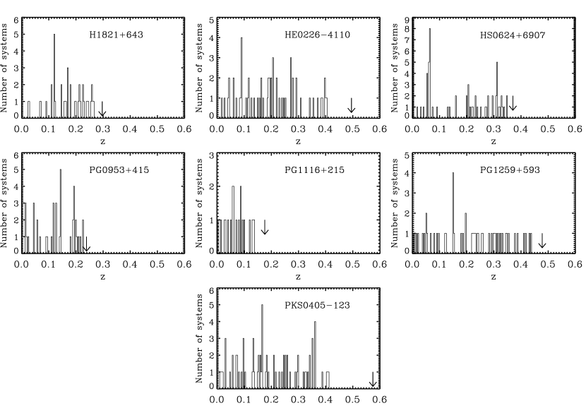
Figure 3.— Distribution of the redshift of H I for each sightline with a redshift interval of $\Delta z=0.0033$. The arrows show the redshifts of the QSOs. The wavelength coverage of the E140M mode of STIS limits Ly$\alpha$ measurements to $z\lesssim 0.42$.

In Fig. 2, we show the distribution of the Doppler parameters for each line of sight and for the entire sample (last panel) with $\sigma_{b}/b,\sigma_{N}/N\leq 0.4$. For every sightline, the $b$-distribution peaks between about 20 and 30 ${\rm km\,s}^{-1}$. Yet, it is apparent that the distribution is not Gaussian around these values, and, in particular, there are many systems with $b\gtrsim 40$–50 ${\rm km\,s}^{-1}$ that produce a tail in the $b$ distribution. This is clearly observed in the histogram of the combined sample where $b$ peaks around 20–30 ${\rm km\,s}^{-1}$ with an excess of systems with $b>40$ ${\rm km\,s}^{-1}$ compared to the number of systems with small $b$. This preview already shows clearly that a mean $b$-value does not provide an adequate description of the Ly$\alpha$ forest.

In Fig. 3, we show the distribution of the redshift for each line of sight with a redshift bin of 0.0033 (corresponding to 1000 ${\rm km\,s}^{-1}$ intervals). There is no striking difference between the different lines of sight, but there are clearly voids and clustering in the distribution, consistent with the Ly$\alpha$ forest tracing filaments of matter in the universe. An example of clustering of absorbers is found near the system at $z=0.06352$ toward HS 0624+6907 where at least 8 absorbers are found in a single bin and 17 absorbers are only separated by about 3000 ${\rm km\,s}^{-1}$. Aracil et al. (2006a) attribute this clustering to the absorption of intragroup gas, possibly from a filament viewed along its long axis.

3. Distribution of the Doppler Parameter

Earlier low-redshift UV studies of the H I forest have low or moderate spectral resolutions and smaller wavelength coverage and did not allow access to several Lyman series transitions. Therefore, the Doppler parameter $b$ generally had to be assumed and a study of the evolution and distribution of $b$ was not possible (see for example the studies of Weymann et al., 1998; Penton et al., 2000, 2004). With STIS E140M observations (spectral resolution of 6.5 ${\rm km\,s}^{-1}$), $b$ can be derived from profile fitting analysis. Furthermore, combining STIS E140M and FUSE observations allows further constraints on $b$ by using several Lyman series lines and reducing possible misidentifications. Here, we review the frequency and properties of the narrow Ly$\alpha$ absorbers (NLAs, $b\leq 40$ ${\rm km\,s}^{-1}$) and the broad Ly$\alpha$ absorbers (BLAs, $b>40$ ${\rm km\,s}^{-1}$).

3.1. Distribution of $b$ and Other Low $z$ Studies

The median $b$-value of 31 ${\rm km\,s}^{-1}$ for our combined sample is larger than the medians found in the low redshift IGM studies by Davé & Tripp (2001) and Shull et al. (2000). Davé & Tripp (2001) used automated software to derive $b$ and $N$, but their criteria did not allow a search for broad components. Shull et al. (2000) went only after the Ly$\beta$ absorption lines in the FUSE wavelength range to combine with known Ly$\alpha$ absorption lines observed with GHRS and were therefore less likely to find the broad H I absorbers. Davé & Tripp (2001) found median and mean $b$-values of 22 ${\rm km\,s}^{-1}$ and 25 ${\rm km\,s}^{-1}$, respectively. We find that the distribution of $b$ is not gaussian, making the mean and dispersion less useful quantities. If we restrict our sample to data with $b\leq 40$ ${\rm km\,s}^{-1}$, the median and mean (with 1$\sigma$ dispersion) are 27 ${\rm km\,s}^{-1}$ and $27\pm 7$ ${\rm km\,s}^{-1}$. If only data with $\log N($H I$)\gtrsim 13.2$ are considered, we obtain 29 ${\rm km\,s}^{-1}$ and $28\pm 6$ ${\rm km\,s}^{-1}$. If we set the cutoff at $b\leq 50$ ${\rm km\,s}^{-1}$, the median and the mean increase by 2 ${\rm km\,s}^{-1}$. The median, mean, and dispersion of $b$ in our sample (with $b\leq 40$ or 50 ${\rm km\,s}^{-1}$) compare well to those derived by Shull et al. (2000): 28 ${\rm km\,s}^{-1}$ and $31\pm 7$ ${\rm km\,s}^{-1}$ for the median and mean, respectively.

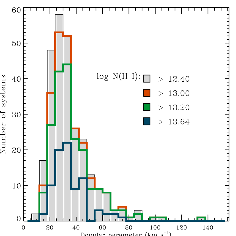
Figure 4.— Distribution of the Doppler parameter of H I for a series of minimum $\log N($H I) for $z\lesssim 0.4$ for the seven sightlines. Only data with less than 40% errors in $b$ and $N_{\rm HI}$ are considered.

In Fig. 4, we show the distribution of $b$ for samples with various $N_{\rm HI}$ cutoffs. For any $N_{\rm HI}$ cutoff, the maximum of the distribution always peaks near 25–30 ${\rm km\,s}^{-1}$ and in all cases there is clearly an asymmetry in the distribution with the presence of a tail in the distribution that develops at $b>40$–60 ${\rm km\,s}^{-1}$. For the BLAs, the number of systems with H I column between 13.0 and 13.2 dex is the largest, although this could be in part an observational bias since weaker column density absorbers with $b>40$ ${\rm km\,s}^{-1}$ would require higher S/N to be detected. Although the effects of line blending can contaminate the measurements of the observed tails, the various papers describing the data (see also Richter et al., 2006b) show that a large fraction of these broad absorbers can be described with a single Gaussian within the S/N. For the stronger of these absorbers, several Lyman series lines were also used to derive the physical parameters.

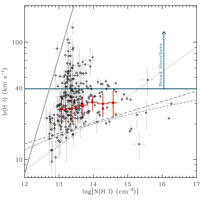
Figure 5.— Line width versus H I column density for the Ly$\alpha$ absorbers along the seven sightlines. Only data with less than 40% errors in $b$ and $N_{\rm HI}$ are considered. The solid gray line shows $b$ vs $N$(H I) for a Gaussian line shape with 10% central optical depth – absorption lines to the left of this line are not detectable. The dotted gray line shows the predicted minimum $b$-value from hydrodynamic cosmological simulations at low redshift (Davé et al., 1999). The dot-dashed and long-dashed lines shows the fits to lower cutoff in the $b$ distribution of high redshift systems (Kirkman & Tytler, 1997; Kim et al., 2002b) (see §3.2 for more details). The red histogram and red symbols show the median $b$ (triangles), the mean and dispersion of $b$ (circles and vertical bars) in six bins of $N_{\rm HI}$ only for data with $b\leq 40$ ${\rm km\,s}^{-1}$ (see Table 3).

3.2. The $b$–$N_{\rm HI}$ distribution

The $b$–$N_{\rm HI}$ distribution of the low redshift sample is shown in Fig. 5. The solid gray line shows the threshold detection of H I absorbers. This curve is the relationship between $b$ and $N_{\rm HI}$ for a Gaussian line profile with 10% central optical depth – absorption lines to the left of this line are not detectable. The lack of data with low $b$ and $\log N_{\rm HI}\lesssim 12.7$ is most likely because our sample is not complete at these low column densities. When absorbers with $\log N_{\rm HI}\gtrsim 13.2$ and $b>0$ ${\rm km\,s}^{-1}$ are considered, the $b$–$N_{\rm HI}$ plot reveals mostly a scatter diagram. Most of the absorbers are present in the column density range 13.2–14 dex. In Table 3, we list the median, mean, and dispersion of $b$ for the entire sample, NLAs, and BLAs. For the entire sample, as expected from Fig. 5, it is not clear if $b$ increases or decreases as $N_{\rm HI}$ increases. A Spearman rank-order correlation test on the entire sample with $\log N_{\rm HI}\geq 13.2$ shows a very marginal negative correlation between $b$ and $N_{\rm HI}$ with a rank-order correlation coefficient $r=-0.08$ and a statistical significance $t=0.25$. We note that when systems with $\log N_{\rm HI}\lesssim 13.2$ are considered, it creates an apparent correlation ($r=0.21$ and $t=4.7\times 10^{-4}$) between $N_{\rm HI}$ and $b$, which can be understood in terms of measurement biases, since weak broad systems are more difficult to detect than weak narrow absorbers. There is no clear separation between the NLAs and BLAs in this figure, although we note that most BLAs are found at $\log N_{\rm HI}\lesssim 14.0$ and no BLAs with $b>50$ ${\rm km\,s}^{-1}$ have $\log N_{\rm HI}\gtrsim 14.0$ (see below). This scatter and absence of clear separation between NLAs and BLAs are expected if the H I lines trace systems with different temperatures and turbulent velocities.

For NLAs with $b\leq 40$ ${\rm km\,s}^{-1}$ and $\log N_{\rm HI}\geq 13.2$, we show in Fig. 5 the median, mean, and dispersion of $b$ (red curves and symbols) derived in six intervals of $N_{\rm HI}$. These estimates are summarized in Table 3. This shows evidence of an increase of $b$ with increasing $N_{\rm HI}$ for the NLAs, at least for the weak absorbers with $\log N_{\rm HI}\lesssim 14.1$. The Spearman rank-order correlation test for the NLA sample shows a weak correlation between $b$ and $N_{\rm HI}$ with $r=0.12$ and $t=0.15$. Since the sample is complete for the NLAs, the increase of $b$ with increasing $N_{\rm HI}$ must be real. The large scatter is again expected if the H I lines are broadened as a result of different temperatures and turbulent velocities.

In Fig. 6, we present the $b$–$N_{\rm HI}$ distribution only for the BLAs (left panel), which shows that $b$ appears to decrease with increasing $N_{\rm HI}$: For $13.1\lesssim\log N_{\rm HI}\lesssim 13.5$ (this range is highlighted in Fig. 6 by the vertical dotted lines), $b$ is distributed between about 40 and 130 ${\rm km\,s}^{-1}$; for $13.5\lesssim\log N_{\rm HI}\lesssim 14.0$, $b$ is mostly distributed between about 40 and 80 ${\rm km\,s}^{-1}$; and for $\log N_{\rm HI}\gtrsim 14.0$, $b$ is always lower than 50 ${\rm km\,s}^{-1}$. This trend is also confirmed in the last two columns of Table 3 (note that in the [13.8,14.1] interval there are only 6 systems, with 3 of them having $b>60$ ${\rm km\,s}^{-1}$ and the other 3 having $b\sim 40$ ${\rm km\,s}^{-1}$). The Spearman rank-order correlation for the BLA sample with $\log N_{\rm HI}\geq 13.2$ confirms a negative correlation between $b$ and $N_{\rm HI}$ ($r=-0.30$ and $t=0.016$).

In the right panel of Fig. 6, we show the recent simulation of BLAs undertaken by Richter et al. (2006a), in which artificial spectra were generated from the hydrodynamical simulation. Their numerical model was part of an earlier investigation of the O VI absorption arising in WHIM filaments (Fang & Bryan, 2001), and they include collisional ionization and photoionization processes. The simulated sample presented in Fig. 6 corresponds to their high-quality sample that includes 321 BLAs with almost perfect Gaussian profiles (note that 58% of the sample has $\log N_{\rm HI}\lesssim 13.2$). Since our observations are complete only to $\log N_{\rm HI}\gtrsim 13.2$, it is not surprising that we are missing absorbers below this limit. It is, however, interesting to note that the simulation and observations have a similar trend: (i) most of the broadest absorbers are found at $\log N_{\rm HI}\lesssim 13.5$, and (ii) most of the strong absorbers ($\log N_{\rm HI}\gtrsim 14$) have $b\lesssim 50$ ${\rm km\,s}^{-1}$ (although we note that in the simulation a few systems have $b$ up to 65 ${\rm km\,s}^{-1}$, and the simulation does not produce BLAs with $\log N_{\rm HI}\gtrsim 14.4$). This is also in general agreement with the simulation of the WHIM produced by Davé et al. (2001) where they show the WHIM fraction peaks for an overdensity $\rho/\bar{\rho}$ of $\sim$$5$–30. If Eq. 2 (see below) applies for the BLAs, the H I column density range $13.2$ to 14.0 dex corresponds to $\rho/\bar{\rho}\sim 5$–17, in general agreement with the hydrodynamical simulations of Davé et al. (2001) if the BLAs trace mostly the WHIM. We note that the simulation of Richter et al. (2006a) generally produces larger $b$ than currently observed: for systems with $\log N_{\rm HI}\gtrsim 13.2$, the median, mean, and standard deviation are 59, 69, 31 ${\rm km\,s}^{-1}$ for the simulation, while they are 52, 57, 18 ${\rm km\,s}^{-1}$ for the observations. The current S/N of the observed data limits the detection of the broader absorbers with $b>80$ ${\rm km\,s}^{-1}$, as discussed in §2. We also note that the broader systems ($b>80$ ${\rm km\,s}^{-1}$) are likely to be more uncertain, especially since they are detected in the lowest column density range ($\log N_{\rm HI}\lesssim 13.4$).

Figure 6.— Left: Line width versus H I column density for the BLAs ($b>40$ ${\rm km\,s}^{-1}$) along the seven sightlines. Only data with less than 40% errors in $b$ and $N_{\rm HI}$ are considered. Right: Line width versus H I column density for the high-quality sample of BLAs simulated by Richter et al. (2006a). The dashed vertical lines highlight the column density range [13.1,13.5] dex where the broadest absorbers with $b>80$ ${\rm km\,s}^{-1}$ are detected in the observational sample.

Schaye et al. (1999) and others demonstrated that the temperature-density relation, which is well described by a power law $T=T_{0}(\rho/\bar{\rho})^{\gamma-1}$ (where $\bar{\rho}$ is the average density, $\rho/\bar{\rho}$ is the overdensity of the IGM), implies a lower envelope to the $b$–$N_{\rm HI}$ distribution. This lower envelope is not clearly observed in Fig. 5. We further explore this by considering the numerical cosmological simulations of the low-redshift Ly$\alpha$ forest that predict that the temperature $T_{4}=T/(10^{4}\,{\rm K})$ is a power law of the overdensity $\rho/\bar{\rho}$, with

$$T_{4}\approx 0.5\left(\frac{\rho}{\bar{\rho}}\right)^{0.6}\,,$$ (1)

for the coolest systems at any given density. The overdensity is connected to the H I column density through (Davé et al., 1999),

$$\frac{\rho}{\bar{\rho}}\approx 20\left(\frac{N_{\rm HI}}{10^{14}\,{\rm cm}^{-2}}\right)^{0.7}\,10^{-0.4z}\,.$$ (2)

Table 3Median, mean, dispersion of $b$ at low $z$ in a given column density interval for the 7 QSO sample

Column	median	mean $\pm\sigma$	median	mean $\pm\sigma$	median	mean $\pm\sigma$
Density interval	$b>0$ ${\rm km\,s}^{-1}$		$b\leq 40$ ${\rm km\,s}^{-1}$		$b>40$ ${\rm km\,s}^{-1}$
$[12.9,13.2]$	28.7	$31.5\pm 13.9$	27.2	$26.7\pm 6.5$	50.7	$54.7\pm 16.6$
$[13.2,13.5]$	34.0	$39.9\pm 21.7$	27.0	$27.2\pm 6.7$	55.4	$61.5\pm 21.1$
$[13.5,13.8]$	32.0	$36.3\pm 12.9$	28.7	$29.1\pm 5.4$	54.1	$53.2\pm 8.4$
$[13.8,14.1]$	34.0	$36.9\pm 14.1$	31.0	$30.7\pm 4.9$	62.0	$57.8\pm 15.7$
$[14.1,14.4]$	37.0	$34.1\pm 9.1$	27.7	$29.8\pm 6.8$	45.7	$45.0\pm 1.2$
$[14.4,14.7]$	39.1	$35.2\pm 8.9$	30.3	$30.5\pm 8.0$	43.0	$43.2\pm 1.3$

Note. — Only data with $\sigma_{b}/b,\sigma_{N}/N\leq 0.4$ are included in the various samples.

If we combine these two equations, we have:

$$T_{4}\approx 3\left(\frac{N_{\rm HI}}{10^{14}\,{\rm cm}^{-2}}\right)^{0.42}\,10^{-0.24z}\,.$$ (3)

The pure thermal Doppler broadening for H is $b_{\rm th}=0.129\sqrt{T}$, so for photoionized hydrogen absorbers we can write

$$b_{\rm th}\approx 22\left(\frac{N_{\rm HI}}{10^{14}\,{\rm cm}^{-2}}\right)^{0.21}\,10^{-0.12z}\,{\rm km\,s}^{-1}\,.$$ (4)

This latter relation is shown in Fig 5 with the dotted line where we set $z=0.2$, which is about the mean and median $z$ in our sample. Since the $\rho$–$T$ fit to photoionized absorbers is for the coolest systems, this relation should provide a lower envelope to the $b$–$N_{\rm HI}$ distribution. The lower envelope to the observed $b$–$N_{\rm HI}$ distribution roughly agrees with the numerical simulations, at least as long as $\log N_{\rm HI}\lesssim 14.2$. But the low redshift sample does not provide yet as sharp a lower envelope to the $b$–$N_{\rm HI}$ distribution as high redshift samples do (see for example Kirkman & Tytler, 1997; Kim et al., 2002a) because there are still too few systems at the completeness level. In Fig. 5, we show with the dot-dashed line the relation $b_{\rm min}=20+4\log[N_{\rm HI}/(10^{14}{\rm cm^{-2}})]$ ${\rm km\,s}^{-1}$ found by Kirkman & Tytler (1997) at $\bar{z}=2.7$ and with the long dashed line the relation $\log b_{\rm min}=1.3+0.090\log[N_{\rm HI}/(10^{14}{\rm cm^{-2}})]$ ${\rm km\,s}^{-1}$ found by Kim et al. (2002b) at $\bar{z}=2.1$ (smoothed power-law fit). These power laws provide a good approximation to the observed lower envelope of $b$ at high redshift. At low redshift at $\log N_{\rm HI}\gtrsim 13.2$, a few absorbers lie below these fits, especially at $\log N_{\rm HI}\gtrsim 15$. For systems with $\log N_{\rm HI}\lesssim 15$ it is not clear if the lower $b$ cutoff evolves with redshift.

Finally, following Davé & Tripp (2001), if we compare the median in the various intervals with $b\leq 40$ ${\rm km\,s}^{-1}$ (red curve in Fig. 5) and $b_{\rm th}$ defined in Eq. 4, we find that $b_{\rm th}\sim(0.6-0.7)b_{\rm obs}$ for a typical absorber with $\log N_{\rm HI}\lesssim 14.2$. Therefore, the contribution from thermal broadening is substantial for the low redshift NLAs. However, if the some BLAs actually trace cool photoionized gas, the non-thermal broadening will be dominant in these absorbers.

3.3. Ly$\alpha$ Line Density

This sample provides the first opportunity to investigate the relative number of systems as a function of the Doppler parameter in the low-$z$ IGM. In Table 4, we summarize $d{\mathcal{N}}/dz$ for each sightline and for the combined sample where our sub-samples have either $b\leq 40$ ${\rm km\,s}^{-1}$ or $b\leq 150$ ${\rm km\,s}^{-1}$. For both $b$-samples, we choose three different column density ranges: (a) $[13.2,14.0]$ dex, (b) $[13.2,16.5]$ dex and (c) $[13.64,16.5]$ dex. The lower limit of samples (a) and (b) corresponds to our threshold of completeness. The largest observed column density in our sample is about $10^{16.5}$ cm^-2. Hence sample (b) corresponds to the combined sample with $W\gtrsim 90$ mÅ, while sample (a) only covers the weaker Ly$\alpha$ lines which may evolve differently than the stronger lines since the weaker lines may arise from tenuous gas in the IGM while the stronger lines may mostly trace the gas in the outskirts of galaxies. The threshold of sample (c) was chosen to be comparable to the equivalent width threshold of 0.24 Å from the HST QSO absorption line key project (Weymann et al., 1998). The last rows of the subtables in Table 7 show the mean $d{\mathcal{N}}/dz$ for the 7 sightlines. We considered only absorbers with $\sigma_{b}/b,\sigma_{N}/N\leq 0.4$. Note that the average values would have increased only by $\sim$5% if we did not apply this cutoff.

Table 4Ly$\alpha$ Line Density

Sightline	${\mathcal{N}}_{\rm HI}$	$d{\mathcal{N}}_{\rm HI}/dz$	${\mathcal{N}}_{\rm HI}$	$d{\mathcal{N}}_{\rm HI}/dz$
	$b\leq 40$ ${\rm km\,s}^{-1}$		$b\leq 150$ ${\rm km\,s}^{-1}$
(a) $13.2\leq\log N_{\rm HI}\leq 14.0$
H 1821+643	7	$29\pm 11$	12	$50\pm 15$
HE 0226–4110	16	$40\pm 10$	22	$55\pm 12$
HS 0624+6907	22	$67\pm 14$	31	$94\pm 17$
PG 0953+415	13	$64\pm 18$	17	$84\pm 20$
PG 1116+215	7	$56\pm 21$	12	$95\pm 28$
PG 1259+593	24	$68\pm 14$	35	$99\pm 17$
PKS 0405–123	21	$51\pm 11$	35	$85\pm 14$
Mean		$54\pm 5(15)$		$80\pm 6(20)$
(b) $13.2\leq\log N_{\rm HI}\leq 16.5$
H 1821+643	9	$38\pm 13$	15	$63\pm 16$
HE 0226–4110	21	$52\pm 11$	31	$77\pm 14$
HS 0624+6907	25	$76\pm 15$	35	$106\pm 18$
PG 0953+415	14	$69\pm 19$	18	$89\pm 21$
PG 1116+215	8	$64\pm 23$	13	$103\pm 29$
PG 1259+593	30	$85\pm 15$	43	$121\pm 19$
PKS 0405–123	33	$80\pm 14$	47	$114\pm 17$
Mean		$66\pm 6(17)$		$96\pm 7(21)$
(c) $13.64\leq\log N_{\rm HI}\leq 16.5$
H 1821+643	6	$25\pm 10$	7	$29\pm 11$
HE 0226–4110	10	$25\pm 8$	16	$40\pm 10$
HS 0624+6907	10	$30\pm 10$	13	$40\pm 11$
PG 0953+415	6	$30\pm 12$	6	$30\pm 11$
PG 1116+215	2	$16\pm 11$	2	$16\pm 11$
PG 1259+593	12	$34\pm 10$	18	$51\pm 13$
PKS 0405–123	16	$39\pm 10$	21	$51\pm 12$
Mean		$28\pm 4(8)$		$37\pm 4(13)$

Note. — Only data with $\sigma_{b}/b,\sigma_{N}/N\leq 0.4$ are included in the various samples. Errors are from Poisson statistics. The number between parentheses in the row showing the mean corresponds to the standard deviation around the mean for the different lines of sight.

The average value of $d{\mathcal{N}}/dz$ in sample (c) ($W\gtrsim 0.24$ Å) of $28\pm 4$ for $b\leq 40$ ${\rm km\,s}^{-1}$ is slightly smaller than the estimates of Weymann et al. (1998) at $\log(1+z)<0.15$ and Impey et al. (1999) at $0<z<0.22$, because the broader absorbers and uncertain absorbers are not included in our sample. Indeed, the estimates of Weymann et al. (1998) and Impey et al. (1999) appear intermediate between our two $b$ samples. Penton et al. (2004) found $d{\mathcal{N}}/dz=25\pm(4,5)$ for a sample with $z<0.069$ which overlaps with our estimate within the 1$\sigma$ dispersion, which implies little or no evolution of $d{\mathcal{N}}/dz$ at $z\lesssim 0.4$ for the strong H I absorbers. For $b\leq 150$ ${\rm km\,s}^{-1}$, the value of $d{\mathcal{N}}/dz$ is about 1.3 times larger than for the NLAs. We find that the broad Ly$\alpha$ lines with $40<b\leq 150$ ${\rm km\,s}^{-1}$ have $d{\mathcal{N}}({\rm BLA})/dz\approx 9$, implying that for the stronger lines of the Ly$\alpha$ forest, the number of BLAs per unit redshift may be important.

Comparison of samples (a) and (b) shows that the weak systems are far more frequent than the strong systems. For these samples, we note that $d{\mathcal{N}}/dz$ is systematically smaller toward H 1821+643 and HE 0226–4110 than $d{\mathcal{N}}/dz$ toward the other sightlines for both $b$ sub-samples. $d{\mathcal{N}}/dz$ toward PG 1116+215 and PKS 0405–123 is intermediate for the NLAs. The 3 other lines of sight have similar $d{\mathcal{N}}/dz$. These trends do not appear related to the S/N of the data since the S/N is the highest toward H 1821+643 and comparatively low for HE 0226–4110. The redshift paths do not seem to explain all the differences. For example, while the redshift paths are comparable between HE 0226–4110 and PG 1259+593, $\Delta z$ is significantly smaller toward PG 1116+215. $d{\mathcal{N}}/dz$ is very similar for either column density range toward the sightlines that cover small and large redshift paths, implying no redshift evolution of $d{\mathcal{N}}/dz$ between $z>0.$ and $z\lesssim 0.4$. Therefore, some of the observed variation in $d{\mathcal{N}}/dz$ must be cosmic variance between sightlines.

We explore the effect of the S/N on the $d{\mathcal{N}}({\rm BLA})/dz$ estimate in Table 5 by considering data with $\sigma_{b}/b,\sigma_{N}/N\leq 0.4$, 0.3, and 0.2. As expected, the spectra with the highest S/N are less affected by these cutoffs than the spectra with the lowest S/N. Decreasing the error thresholds has an effect mostly on the weak systems ($\log N_{\rm HI}\lesssim 13.40$). Toward PG 0953+415, the four BLAs have $13.2<\log N_{\rm HI}\leq 13.40$ and $0.23\leq\sigma_{b}/b\leq 0.30$, which explains why there is no BLA at the threshold $\sigma_{b}/b\leq 0.2$. Although the HS 0624+6207 spectrum has several weak BLAs, only if $\sigma_{b}/b,\sigma_{N}/N<0.15$ is applied do we observe a significant drop in $d{\mathcal{N}}({\rm BLA})/dz$ by a factor 2.5. On average, there is a decrease in $d{\mathcal{N}}({\rm BLA})/dz$ by a factor $\sim$1.4 between the cutoff at 0.4 and 0.2. If only BLAs with $40<b\leq 100$ ${\rm km\,s}^{-1}$ are considered, $d{\mathcal{N}}({\rm BLA})/dz=28,25,20$ for $\sigma_{b}/b,\sigma_{N}/N\leq 0.4,0.3,0.2$, respectively. These estimates are in agreement with those of Richter et al. (2006b) (see also §4.2). The BLA density is about twice smaller than $d{\mathcal{N}}({\rm NLA})/dz$ for samples (a) and (b).

Table 5Effect of the Signal-to-Noise on the Broad Ly$\alpha$ Density Estimate

Sightline	S/N	$d{\mathcal{N}}_{\rm HI}/dz$	$d{\mathcal{N}}_{\rm HI}/dz$	$d{\mathcal{N}}_{\rm HI}/dz$
		$\sigma_{b}/b\leq 0.4$	$\sigma_{b}/b\leq 0.3$	$\sigma_{b}/b\leq 0.2$
		$\sigma_{N}/N\leq 0.4$	$\sigma_{N}/N\leq 0.3$	$\sigma_{N}/N\leq 0.2$
H 1821+643	15–20	$25\pm 10$	$25\pm 10$	$25\pm 10$
HE 0226–4110	5–11	$25\pm 8$	$20\pm 7$	$18\pm 7$
HS 0624+6907	8–12	$30\pm 10$	$30\pm 10$	$30\pm 10$
PG 0953+415	7–11	$20\pm 10$	$15\pm 9$	0
PG 1116+215	10–15	$40\pm 18$	$40\pm 18$	$32\pm 16$
PG 1259+593	9–17	$37\pm 10$	$34\pm 10$	$25\pm 9$
PKS 0405–123	5–10	$34\pm 9$	$24\pm 8$	$14\pm 6$
Mean		$30\pm 4(7)$	$27\pm 4(8)$	$21\pm 3(11)$

Note. — S/N is measured per resolution element. Sample with $40<b\leq 150$ ${\rm km\,s}^{-1}$ and $13.2\leq\log N_{\rm HI}\leq 16.5$. Errors are from Poisson statistics. The number between parentheses in the row showing the mean corresponds to the standard deviation around the mean for the different lines of sight.

Finally, we summarize in Fig. 7 the frequency of the Ly$\alpha$ absorbers with various $b$-values in the low redshift universe. In this figure, $d{\mathcal{N}}/dz$ represents the mean of the number density of H I absorbers obtained toward each line of sight in four intervals of $b$ ($[0,20]$, $[20,40]$, $[40,60]$, $[60,80]$ ${\rm km\,s}^{-1}$) using data with $\sigma_{b}/b,\sigma_{N}/N\leq 0.4$ and $\log N_{\rm HI}\geq 13.2$. The vertical error bars assume Poissonian errors. The mean $d{\mathcal{N}}/dz$ is shown at the mean $b$-value of each $b$-interval sample. The horizontal bars show the $b$-intervals delimited by the minimum and maximum $b$-values of each $b$-interval sample. The NLAs are mostly found between 20 and 40 ${\rm km\,s}^{-1}$. Very narrow Ly$\alpha$ absorbers with $b<20$ ${\rm km\,s}^{-1}$ are rare, and we note that in the $[0,20]$ ${\rm km\,s}^{-1}$ interval, most of the absorbers have $b\gtrsim 15$ ${\rm km\,s}^{-1}$. The paucity of very narrow absorbers with $\log N_{\rm HI}\geq 13.2$ is real since the resolution of STIS E140M ($b_{\rm inst}\sim 4$ ${\rm km\,s}^{-1}$) allows to fully resolve absorbers with $b\gtrsim 5$ ${\rm km\,s}^{-1}$. The broad absorbers are more frequent in the $b=[40,60]$ ${\rm km\,s}^{-1}$ range: there are about 3.5 times more absorbers in $[40,60]$ ${\rm km\,s}^{-1}$ interval than in the $b=[60,80]$ ${\rm km\,s}^{-1}$ interval. Ly$\alpha$ absorbers are therefore more frequent for low column densities ($\log N($H I$)\lesssim 14$) and for $b$-values between 20 and 40 ${\rm km\,s}^{-1}$.

Figure 7.— Mean number density per unit redshift with Poissonian errors (vertical bars) in four intervals of $b$ ($[0,20]$, $[20,40]$, $[40,60]$, $[60,80]$ ${\rm km\,s}^{-1}$) using data with $\sigma_{b}/b,\sigma_{N}/N\leq 0.4$ and $\log N_{\rm HI}\geq 13.2$. The mean number density is shown at the mean $b$-value of each $b$-interval sample. The horizontal bars show the $b$-intervals delimited by the minimum and maximum $b$-values of each $b$-interval sample.

4. Evolution of the Doppler Parameter

4.1. Higher Redshift Samples

Recently, the analysis of the Ly$\alpha$ absorbers in the redshift range $0.5<z<2.0$ from Janknecht et al. (2006) has become available at the Centre de Données de Strasbourg (CDS). Their data that sample the mid-$z$ IGM at $0.5<z\lesssim 1.5$ were obtained with HST/STIS E230M: PG 1634+706 ($z=0.534$–1.295), PKS 0232–04 ($z=0.876$–1.419), PG 1630+377 ($z=0.875$–1.451), PG 0117+213 ($z=0.875$–1.475), HE 0515–4414 ($z=0.874$–1.475) and HS 0747+4259 ($z=0.760$–1.443). The redshifts between parentheses indicate the redshift interval probed by the observations. The spectral resolution of E230M data ($R\sim 30000$) is lower than that of the low-$z$ sample obtained with the E140M grating ($R\sim 44000$). The S/N of the mid-$z$ sample is comparable to the lowest S/N of the low-$z$ sample, except for PG 1634+706, which has a S/N per resolution element of 5–40. The high redshift sample ($z>1.5$) consists of data obtained with VLT/UVES ($R\sim 40000$): HE 0515–4414 (1.515–1.682), HE 0141–3932 ($z=1.518$–1.784), HE 2225–2258 ($z=1.515$–1.861), and HE 0429–4901 ($z=1.662$–1.910). The S/N is typically higher than 30–40, except for HE 0429–4901, which is about 15. The spectrum of HS 0747+4259 ($z=1.562$–1.866) was also obtained with Keck/HIRES ($R\sim 50000$) with a S/N in the range of 6–24.

For the high redshift sample, we also consider the spectra of QSOs at $z>1.5$ presented by Kim et al. (2002a). Their profile fitting results are available at the CDS. These data were obtained with the VLT/UVES at resolution of $R\sim 45000$ and typical S/N $\simeq 40$–50. The QSOs considered are: HE 0515–4414 ($z=1.53$–1.69), Q 1101–264 ($z=1.66$–2.08), J 2233–606 ($z=1.80$–2.20), HE 1122-1648 ($z=1.88$–2.37), HE 2217–2818 ($z=1.89$–2.37), HE 1347–2457 ($z=2.09$–2.57), Q 0302–003 ($z=2.96$–3.24), Q 0055–269 ($z=2.99$–3.60). Note that the HE 0515–4414 VLT spectrum in Janknecht et al. (2006) has a different wavelength coverage and exposure time than the HE 0515–4414 VLT spectrum presented by Kim et al. (2002a). We finally consider the H I parameters measured toward HS 1946+7658 ($z=2.43$–3.05) by Kirkman & Tytler (1997). The spectrum of HS 1946+7658 was obtained with Keck/HIRES. The S/N per resolution element varies from about 30 to 200 and the spectral resolution is similar to UVES. The spectral resolution of the high redshift sample is similar to the low redshift sample, but the S/N is generally much higher in the $z>1.5$ sample than in the low or mid $z$ samples

4.2. Conditions for Comparing Various Samples

The definition of a BLA that was followed in recent papers presented by our group is an absorber that can be fitted with a single Gaussian component with $b>40$ ${\rm km\,s}^{-1}$ and for which the reduced-$\chi^{2}$ does not improve statistically by adding more components in the model. Low S/N data can have, however, treacherous effects that can mask a BLA or confuse narrow multi-absorbers with a BLA (see Figure 2 in Richter et al. 2006b). To overcome the effects of noise, the sample of BLAs defined by Richter et al. (2006b) has also to satisfy the following rules: (i) the line does not show any asymmetry, (ii) the line is not blended, (iii) there is no evidence of multiple components in the profile; (iv) the S/N must be high enough (i.e. $\log(N_{\rm HI}/b)\gtrsim\log[3\times 10^{12}/({\rm S/N})]\gtrsim 11.3$, where $N_{\rm HI}$ and $b$ are in cm^-2 and ${\rm km\,s}^{-1}$, respectively). For the low redshift sample presented here, the BLAs strictly follow criteria (iv) when the condition $\sigma_{b}/b,\sigma_{N}/N\leq 0.4$ is set.. Following these rules, Richter et al. (2006b) found $d{\mathcal{N}}({\rm BLA})/dz=22\pm 5$ for their secure detections (53 for the entire candidate sample). Within $1\sigma$, our BLA number density estimate overlaps with the result of Richter et al. (2006b) when the cutoff $\sigma_{b}/b,\sigma_{N}/N\leq 0.4$ is applied to our sample. Therefore, this shows that by applying an error cutoff without scrutinizing each profile for the conditions listed above, we find a similar average $d{\mathcal{N}}({\rm BLA})/dz$. This is crucial because for a comparison with other samples at higher $z$, we can not examine each absorber individually. For the sample presented by Janknecht et al. (2006), no spectra or fits are shown. Kim et al. (2002a) and Kirkman & Tytler (1997) present their spectra and fits, but over too broad wavelength ranges to study in detail the conditions listed above. Furthermore, as $z$ increases absorbers are more often blended due to the higher redshift line density, so we can not reject the blended systems, otherwise we would introduce a strong bias in the comparison. At high, mid, and low redshift, the $\chi^{2}$ of the profile fit governs the number of components allowed in the model of an absorber; therefore a similar methodology was applied in each sample, allowing a direct comparison of the various measurements. We apply the same cutoff $\sigma_{b}/b,\sigma_{N}/N\leq 0.4$ to the $z>0.5$ redshift samples to remove the uncertain profile fit results in a similar manner in each sample. Such cutoff, however, introduces a systematic effect: more BLAs will be rejected in low S/N spectra (low and some mid $z$ data) than in high S/N spectra (high $z$ data). But such systematics should underestimate the number of BLAs in low S/N data, and therefore this should strengthen the differences observed at low $z$ compared to the higher $z$ samples.

For our comparison, we also consider only absorbers with $\log N_{\rm HI}\geq 13.2$, the completeness level of the low redshift sample, which also corresponds to about the completeness of the lowest S/N spectra of the mid-$z$ sample. If the S/N of the high redshift spectra is solely considered, absorbers with $\log N_{\rm HI}\geq 13.2$ would be far above the completeness level of the high redshift sample, which is $\log N_{\rm HI}\gtrsim 12.5$ for the data presented by Kim et al. (2002a) and Kirkman & Tytler (1997). However, line blending and blanketing reduce the completeness threshold, especially at $z\gtrsim 2.5$ (Kirkman & Tytler, 1997; Lu et al., 1996). At $z\sim 4$, Lu et al. (1996) show using simulated spectra that line blanketing was not important as long as $\log N_{\rm HI}\gtrsim 13.5$, while at $z\sim 2.7$, Kirkman & Tytler (1997) show following a similar methodology that their sample is likely to be complete at $\log N_{\rm HI}\gtrsim 12.8$–13.0. Since broad and shallow absorbers are more uncertain, considering only absorbers with $\log N_{\rm HI}\geq 13.2$ also reduces the problem of creating a higher proportion of wide lines than is really present in the intrinsic distribution.

For our comparison, we only consider BLAs with $40<b\leq 100$ ${\rm km\,s}^{-1}$. The choice of $b\leq 100$ ${\rm km\,s}^{-1}$ reduces the incompleteness at the high $b$ end of the low redshift sample. Furthermore, at $z\sim 4$ (which is at higher redshift than any absorbers considered here), Lu et al. (1996) argue that absorbers with $b>100$ ${\rm km\,s}^{-1}$ are caused essentially by heavily blended forest lines since they are systematically found in the high line density region of the spectrum. This effect should diminish greatly as $z$ decreases. At $z\sim 2.7$, Kirkman & Tytler (1997) have produced simulated spectra to better understand the intrinsic properties of their observational data. They observe a tail at high $b$ in both the simulated and observed $b$ distributions. In the simulated spectra, the tail at $b>80$ ${\rm km\,s}^{-1}$ is only due to line blending because their simulation did not allow such broad lines. They find more lines at $b>80$ ${\rm km\,s}^{-1}$  in the observed distribution (3.6% compared to 0.5% in the simulated spectra), suggesting that many of these absorbers could be intrinsically broad. Refined simulations, so that simulated observations match exactly the real observations, would be needed to be entirely conclusive on this point (Kirkman & Tytler, 1997). Yet, at high $z$, if BLAs with $b>80$ ${\rm km\,s}^{-1}$ that are in fact blended narrow lines were frequent, this effect should be more important as $z$ increases. We will see that this effect, if present, is not statistically significant (see next two sections). By considering only absorbers with $40<b\leq 100$ ${\rm km\,s}^{-1}$, $\log N_{\rm HI}\geq 13.2$, and $\sigma_{b}/b,\sigma_{N}/N\leq 0.4$, we reduce significantly the risk of including spurious broad absorbers. We also note that, in any samples considered, the majority of BLAs are actually found in the $b$-range $40<b\leq 60$ ${\rm km\,s}^{-1}$, not in the $b$-range $b>80$ ${\rm km\,s}^{-1}$.

Figure 8.— Left panel: Line width versus H I column density for the Ly$\alpha$ absorbers for $13.2\leq\log N_{\rm HI}\leq 16.5$ and $0<b\leq 100$ ${\rm km\,s}^{-1}$ in different redshift intervals indicated in the upper-right corner. Only data with less than 40% errors in $b$ and $N_{\rm HI}$ are considered. The symbols have the following meaning: data represented by circles were estimated from the low redshift sample (see Table 1 for the references); data represented by stars are from the sample of Janknecht et al. (2006); data represented by triangles are from the sample of Kim et al. (2002a); data represented by squares are from the sample of Kirkman & Tytler (1997). Right panel: Same as the left-hand side, but only for absorbers with $13.2\leq\log N_{\rm HI}\leq 14.0$

In Fig. 8, we show the $b$–$N_{\rm HI}$ distribution for three redshift intervals, $z<0.5$ (top panel), $0.5<z<1.5$ (middle panel), and $1.5<z\lesssim 3.6$ (bottom panel). Only absorbers that satisfy the conditions $0<b\leq 100$ ${\rm km\,s}^{-1}$, $\log N_{\rm HI}\geq 13.2$, $\sigma_{b}/b,\sigma_{N}/N\leq 0.4$ are shown in the figure. At $z>0.5$, there are many weak systems with $b<40$ ${\rm km\,s}^{-1}$, which darkens part of the middle and bottom panels. At $z<0.5$, there are very few absorbers with $b\gtrsim 40$ ${\rm km\,s}^{-1}$ and $\log N_{\rm HI}>14$, and none of them have $b>50$ ${\rm km\,s}^{-1}$. This contrasts remarkably with what is observed at higher redshifts: many absorbers at $z>0.5$ have $b>40$ ${\rm km\,s}^{-1}$ and $\log N_{\rm HI}\geq 14.0$. This effect must be due to strong, saturated Ly$\alpha$ lines for which the errors for $b$ and $\log N_{\rm HI}$ are far too optimistic. At $z<0.5$, saturation can be dealt with because higher Lyman series lines are systematically used in the profile fitting, reducing the possibility of non-uniqueness in the profile fitting solution and of finding unrealistic large $b$-values for strong lines. At $z>0.5$, Ly$\alpha$ is generally the only transition available, although we note Kim et al. (2002a) analyzed the Ly$\beta$ forest at $z<2.5$ with a small sample and their results suggested that line blending and saturation are not an important issue. Yet, Fig. 8 shows a system with $b=97.0\pm 3.8$ ${\rm km\,s}^{-1}$ and $\log N_{\rm HI}=16.44\pm 0.14$. This absorber is observed in the spectrum of J 2233–606 at $z=1.869$, and the parameters that are presented here were estimated by Kim et al. (2002a). The spectrum of J 2233–606 is shown in Cristiani & D’Odorico (2000) and at the wavelength corresponding to this absorber, there is a strong, saturated line that Kim et al. (2002a) model with a single component. D’Odorico & Petitjean (2001) actually found that this absorber has $\sim$11–16 components using higher Lyman series lines and metal lines. While this example is extreme, most of the absorbers with $\log N_{\rm HI}>14$ and $b>40$ ${\rm km\,s}^{-1}$ are likely to be strong saturated Ly$\alpha$ lines at $z>0.5$. Fig. 1 in Kirkman & Tytler (1997), which shows the whole HS 1946+7658 spectrum with the values of $\log N_{\rm HI},b$, corroborates this conclusion. The strong, saturated Ly$\alpha$ lines are unlikely to probe a single broad line, but are likely composed of several unresolved components. Therefore, for our comparison, we will consider absorbers with $13.2\leq\log N_{\rm HI}\leq 14.0$. This sample is summarized in the right-hand side of Fig. 8.

As we have just illustrated, the Voigt profile fitting method adopted for deriving $z,b,N_{\rm HI}$ may not be unique, especially for highly blended regions, strong lines, and low S/N spectra. We believe that some of this effect is reduced by considering absorbers with $13.2\leq\log N_{\rm HI}\leq 14.0$, $b<100$ ${\rm km\,s}^{-1}$, and $\sigma_{b}/b,\sigma_{N}/N\leq 0.4$. At low $z$, line blending and strong lines are not a major issue because often higher Lyman series lines can be used. Futhermore, several persons analyzed these data independently, and other methods (curve-of-growth and/or optical depth method) were also used for the low-$z$ sample, yielding consistent results (see the references given in Table 1), although the Appendix highlights some differences between various groups. Even in this latter case, there is roughly a 1$\sigma$ consistency between the various results for absorbers with $13.2\leq\log N_{\rm HI}\leq 14.0$. At $z\sim 2.7$, Kirkman & Tytler (1997) show that profile fitting may not provide a unique solution even in very high S/N data. Yet, their comparison with simulated spectra show that the intrinsic distribution of $b$ is very similar to the observed $b$ distribution. Therefore, in a statistical sense, the observed $b$ distribution at high $z$ can be used for our comparison. We also note that three different research groups have worked on the absorbers at $z\gtrsim 1.5$ presented here, with the spectra obtained from different telescopes with different S/N, and we did not find any major differences between their results, at least within the conditions listed above.

Continuum placement may also be a problem for finding or defining a BLA. At low $z$, BLAs may be confused with continuum undulations. With our constraints, most of these ill-defined BLAs are rejected (see also Richter et al., 2006b). We believe that this conclusion should apply to the mid-$z$ sample, but since Janknecht et al. (2006) did not present any of the spectra they analyze, we treat this sample with more caution (see also below). At $z>1.5$, the continuum is more difficult because each order must be fitted with a high order Legendre polynomial, and during the Voigt profile fitting process, the continuum level is often adjusted to give an optimum fit between the data and the calculated Voigt model. Furthermore, as $z$ increases the continuum placement becomes more difficult because the line density increases, and therefore the line blending and blanketing effects increase. High order polynomials and adjusted continua can therefore mask broad and shallow BLAs. However, such effects may be counterbalanced by a possible spurious increase of BLAs caused by the same line blending and blanketing effects (see above). The high S/N of the data at high redshifts and considering only the absorbers with $13.2\leq\log N_{\rm HI}\leq 14.0$ and $b\leq 100$ ${\rm km\,s}^{-1}$ reduce greatly the risk of losing many BLAs because of the line blending and blanketing at high $z$. The problem of not finding BLAs is potentially more important in the highest $z$ spectra, but we do not notice significant differences between $z\sim 2$ and $z>3$. We also note above that simulated spectra show that line blanketing was not important at $\log N_{\rm HI}\gtrsim 13.2$. Therefore, for the samples considered here using the limits $\log N_{\rm HI}\geq 13.2$ and $b\leq 100$ ${\rm km\,s}^{-1}$, they must almost be complete. Ultimately, one would like to produce simulated spectra of various $z$ with realistic inputs to fully consider the impacts of S/N, continuum placement, and line blending and blanketing on finding BLAs and deriving their intrinsic properties.

Table 6Evolution of $b$

	$z<0.5$	$0.5<z<1.0$	$1.0<z<1.5$	$1.5<z<2.0$	$1.5<z<3.6$	$2.4<z<3.1$
	(this paper)	(J06)	(J06)	(J06)	(K02)	(KT97)
$0<b\leq 100$ ${\rm km\,s}^{-1}$
$b$ median ($m_{\rm tot}$)	30.5 (336)	27.9 (263)	28.3 (588)	28.0 (450)	24.8 (2305)	27.1 (452)
$b$ mean $\pm\sigma$	$34.0\pm 16.9$	$32.9\pm 17.8$	$31.8\pm 17.0$	$31.4\pm 14.5$	$27.2\pm 13.5$	$31.2\pm 16.2$
$m(b>40)/m_{\rm tot}$	0.277	0.274	0.240	0.204	0.131	0.210
$0<b\leq 100$ ${\rm km\,s}^{-1}$ and $0<(\sigma_{b}/b,\sigma_{N}/N)\leq 0.4$ and $13.2\leq\log N_{\rm HI}\leq 14.0$
$b$ median ($m_{\rm tot}$)	32.7 (162)	31.5 (82)	30.8 (209)	28.2 (154)	25.5 (509)	27.1 (123)
$b$ mean $\pm\sigma$	$37.4\pm 16.1$	$36.0\pm 18.3$	$35.5\pm 17.3$	$31.7\pm 12.9$	$29.2\pm 11.9$	$32.5\pm 16.0$
$m(b>40)/m_{\rm tot}$	0.321	0.317	0.272	0.169	0.132	0.179

Note. — Median and mean values of $b$ are listed for the different redshift intervals for the entire samples with $0<b\leq 100$ ${\rm km\,s}^{-1}$ and the higher quality samples restricted to absorbers with $13.2\leq\log N_{\rm HI}\leq 14.0$. $m_{\rm tot}$ is the total number of absorbers in the sample. $m(b>40)$ is the total number of absorbers with $40<b\leq 100$ ${\rm km\,s}^{-1}$ in the sample. The values of $\sigma$ listed are the standard deviation around the mean. Source of profile fitting measurements: J06: Janknecht et al. (2006); K02: Kim et al. (2002a); KT97: Kirkman & Tytler (1997).

The redshift range $z=0.5$–1.5 is more problematic than the other redshift ranges because most of the data have low S/N, all have lower resolution than the higher or lower redshift spectra, and no spectra or fits were presented by Janknecht et al. (2006) making it more difficult to assess some of the issues discussed above. Ly$\beta$ lines are only available for about half the wavelength coverage of this redshift range and lower spectral resolution and S/N of these data further worsen the problems of saturation and non-uniqueness in the profile fitting results. Setting the conditions $0<b\leq 100$ ${\rm km\,s}^{-1}$, $13.2\leq\log N_{\rm HI}\leq 14.0$, and $\sigma_{b}/b,\sigma_{N}/N\leq 0.4$ make this sample stronger, but we nonetheless treat the results from this sample with caution. We will consider two sub-samples for the estimate of the redshift density based on the Janknecht et al. (2006) sample (see §4.4): one with all their data, and one with only their highest S/N data (i.e. PG 1634+706, HE 0515–4144, HE 0141–3932, HE 2225–2258). Among the high S/N data in the mid-$z$ sample are E230M spectra of PG 1634+706 and HE 0515–4144.

For the reasons aforementioned, with the conditions $0<b\leq 100$ ${\rm km\,s}^{-1}$, $13.2\leq\log N_{\rm HI}\leq 14.0$, and $\sigma_{b}/b,\sigma_{N}/N\leq 0.4$, we greatly reduce some pitfalls in comparing data analyzed by various groups, with different S/N, obtained with various instruments, with different line blending issues. A BLA is therefore defined here as an absorber that is fitted with a single Gaussian for which the $\chi^{2}$ does not drop significantly by adding more components (this condition was adopted by the various groups who analyzed the data used here) and that has $40\leq b\leq 100$ ${\rm km\,s}^{-1}$, $13.2\leq\log N_{\rm HI}\leq 14.0$, and $\sigma_{b}/b,\sigma_{N}/N\leq 0.4$. We believe that we are statistically comparing the intrinsic properties of the broadening of H I absorbers, although we note that simulated spectra probing various $z$, with realistic inputs may be the only way to fully understand some of the effects discussed above and how these effects balance each other at various $z$.

4.3. Comparison of the Distributions of $b$ at Low and Higher $z$

Table 6 summarizes the $b$-value median, mean, dispersion, and fraction of BLAs (i.e. systems with $40<b\leq 100$ ${\rm km\,s}^{-1}$). In this table, we consider two sub-samples with $0<b\leq 100$ ${\rm km\,s}^{-1}$: (a) the entire sample, (b) the higher quality sample with $13.2\leq\log N_{\rm HI}\leq 14.0$ and errors in $b$ and $N_{\rm HI}$ less than 40%. We note that the number of systems in each sample is roughly similar, except for the Kim et al. (2002a) sample, which is noticeably larger, and the $0.5<z<1.0$ sample, which is somewhat smaller. In sample (a) there appears to be an increase in the median, mean, and the fraction of BLAs as $z$ decreases. The same trend is observed in sample (b), but the differences are better revealed, where the median and mean are always larger by 15–30% in the low redshift sample ($z<0.5$) than in the high redshift sample ($z>1.5$). For the sample (b), the fraction of BLAs at $z\lesssim 0.4$ is 1.9–2.4 times larger than the fraction of BLAs at $z\gtrsim 1.5$. Therefore, $b$ is larger on average at $z\lesssim 1.0$ than at $z\gtrsim 1.5$, and the fraction of BLAs is larger at $z<1.5$ than at $z>1.5$.

In Figs. 9–12 we compare the distributions of $b($H I). In all comparisons we restrict the observations to the higher quality measurements with less than 40% errors in $b$ and $N_{\rm HI}$.

In Fig. 9, we compare the normalized number distribution of $b$(H I) for the low redshift sample with the normalized number distribution of $b$(H I) for the Janknecht et al. (2006) sample, which is subdivided in 3 $z$ sub-samples. The distributions peak at about $b\sim 20$–30 ${\rm km\,s}^{-1}$. Each distribution shows a tail at higher $b$. The tail in the $1.5<z<2.0$ distribution is always weaker than in the lower $z$-interval distributions, especially for $40<b<55$ ${\rm km\,s}^{-1}$. The tail in the $0.5<z<1.0$ distribution is generally stronger than any other $z$-interval distribution presented in this figure, which is possibly due to a combination of blending effects, low S/N spectra, and lower resolution spectra in the redshift range $0.5<z<1.0$. We note that data probing the redshift ranges $0.5<z<1.0$ and $1.0<z<1.5$ were obtained with the STIS E230M grating, but the sensitivity of E230M is lower for Ly$\alpha$ in the redshift range $0.5\lesssim z\lesssim 0.9$ than $0.9\lesssim z\lesssim 1.4$. A Kolmogorov-Smirnov test does not reveal a significant difference between the samples $z<0.5$ and $0.5<z<1.5$ (the maximum deviation between the two cumulative distributions is $D=0.118$ with a level of significance $P=0.104$), but suggests a difference between the samples $z<0.5$ and $1.5<z<2.0$. Therefore, BLAs appear more frequent at $z<1.5$ than at $z>1.5$.

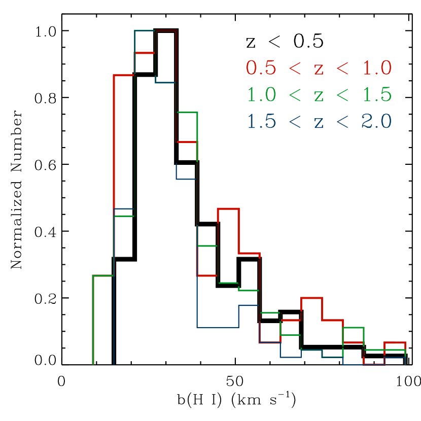
Figure 9.— Comparison of the normalized distributions of $b$(H I) for the low $z$ sample (black histogram) and for the higher $z$ sample (colored histograms) of Janknecht et al. (2006) for the weak absorbers $13.2\leq\log N_{\rm HI}\leq 14.0$. The sample in the redshift range $z\simeq 0.5$–1.5 has a spectral resolution of about 10 ${\rm km\,s}^{-1}$, while the other samples have about 7–8 ${\rm km\,s}^{-1}$. Only data with less than 40% errors in $b$ and $N_{\rm HI}$ are considered.

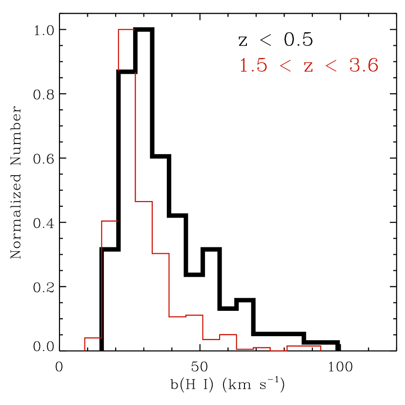
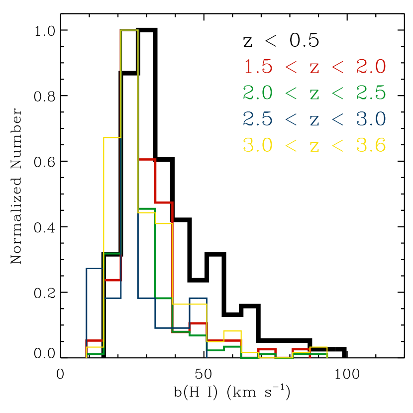
Figure 10.— Left panel: Comparison of the normalized distributions of $b$(H I) for the low $z$ sample of data points (black histogram) and for the high redshift sample (red histogram) from Kim et al. (2002a) for the weak absorbers $13.2\leq\log N_{\rm HI}\leq 14.0$. Right panel: Same as the left panel but the sample of Kim et al. (2002a) is separated in various redshift intervals. Each sample has a similar spectral resolution of about 7–8 ${\rm km\,s}^{-1}$. Only data with less than 40% errors in $b$ and $N_{\rm HI}$ are considered for the different samples.

In Fig. 10, we compare the normalized number distribution of $b$(H I) for the low redshift sample with the normalized number distribution of $b$(H I) for the high redshift sample ($1.5\leq z\leq 3.6$) from Kim et al. (2002a). The left panel shows the entire sample at $1.5\leq z\leq 3.6$, while the right panel shows the distribution of $b$ in various redshift intervals for the high $z$ sample. The peak of the high redshift normalized distribution in Fig. 10 is not only shifted by $\sim-5$ ${\rm km\,s}^{-1}$ with respect to the peak of the low redshift distribution, but also the width of the distribution is smaller for the high redshift sample. Moreover, the low redshift sample shows a tail of high $b$(H I) absorbers that is much weaker in the high redshift sample, showing that BLAs are more frequent at $z<0.5$ than at $z>1.5$. The right-hand side of Fig. 10 verifies this conclusion for the various redshift intervals, i.e. BLAs appear more frequent at $z<0.5$ than for any redshift intervals at $z>1.5$. There is, however, no major difference between the various redshift intervals at $z>1.5$. We also note that the $b$ distribution at $z>1.5$ shows little effect of line blending as $z$ increases since there is scant evidence of a larger of fraction of BLAs at $z\gtrsim 3$ than at $1.5\lesssim z\lesssim 2$.

We compare in Fig. 11 our low $z$ sample to the high redshift absorbers observed toward the QSO HS 1946+7658 (Kirkman & Tytler, 1997). The median and mean are somewhat intermediate between our sample and the Kim et al. (2002a) sample (see Table 6). We slightly adjusted the redshift of the low $z$ sample so that the low and high redshift samples have exactly the same number of systems ($m=130$); hence the two distributions can be directly compared. The peak of the high redshift distribution in Fig. 10 is again shifted by $\sim-5$ ${\rm km\,s}^{-1}$ with respect to the peak of the low $z$ distribution. A higher number of systems with $40<b\leq 70$ ${\rm km\,s}^{-1}$ is found in the low redshift sample. At $b>70$ ${\rm km\,s}^{-1}$ the high redshift sample appears to have a larger number of systems. However, we note that the data of Kirkman & Tytler (1997) have S/N  up to 200, and as we discussed in §2 our sample is not complete for $b>80$ ${\rm km\,s}^{-1}$. A Kolmogorov-Smirnov test yields a maximum deviation between the two cumulative distributions of the low and high redshift samples $D=0.210$ with a level of significance $P=0.006$; the null hypothesis of no difference between the two datasets is therefore rejected.

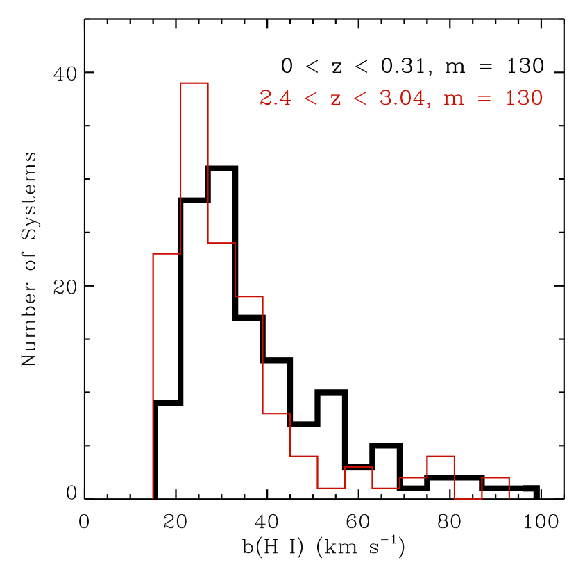
Figure 11.— Comparison of the distributions of $b$(H I) for the low $z$ STIS E140M sample (black histogram) and for the high $z$ Keck sample (red histogram) of Kirkman & Tytler (1997) for the weak absorbers $13.2\leq\log N_{\rm HI}\leq 14.0$. The number of absorbers in each sample is the same: $m=130$. Only data with less than 40% errors in $b$ and $N_{\rm HI}$ are considered for both samples.

So far, we have ignored the effects of evolution of column density in the absorbers in our comparison. According to the numerical simulation of Davé et al. (1999), the dynamical state of an absorber depends mainly on its overdensity, so that a column density range traces absorbers of progressively higher overdensity as the universe expands. Therefore, according to Eq. 2, a low redshift H I absorber is physically analogous to a high redshift H I absorber not with the same column density but to an absorber with column density $10^{0.4\times(z_{\rm high}-z_{\rm low})/0.7}$ times higher (Davé et al., 1999). With the average redshifts of 2.6 and 0.2 of the high redshift sample of Kim et al. (2002a) and our sample, this corresponds to a column density roughly 25 times higher, i.e. a sample with $12.5\leq\log N_{\rm HI}\leq 14.1$ at low $z$ is physically analogous to the high redshift sample with $13.9\leq\log N_{\rm HI}\leq 15.5$. At such high column density, BLAs are likely to trace in large part narrower, strong absorbers that are blended together (see §4.2). We, nonetheless, make this comparison in Fig. 12, where both samples have the same number of systems. The high redshift sample has again a larger fraction of systems in the range $b=[20,40]$ ${\rm km\,s}^{-1}$ than the low redshift sample. The fraction of BLAs at low redshift is again larger than the fraction of BLAs at high redshift with $b>50$ ${\rm km\,s}^{-1}$. This is remarkable since the low redshift sample is far from complete for $\log N_{\rm HI}\lesssim 13.2$ and the high redshift sample likely overestimates the number of true BLAs (i.e. BLAs that are not blends of NLAs). We again apply a Kolmogorov-Smirnov test on the two cumulative distributions of the low and high redshift samples and find $D=0.130$ with a level of significance $P=0.029$; again the null hypothesis of no difference between the two datasets is rejected.

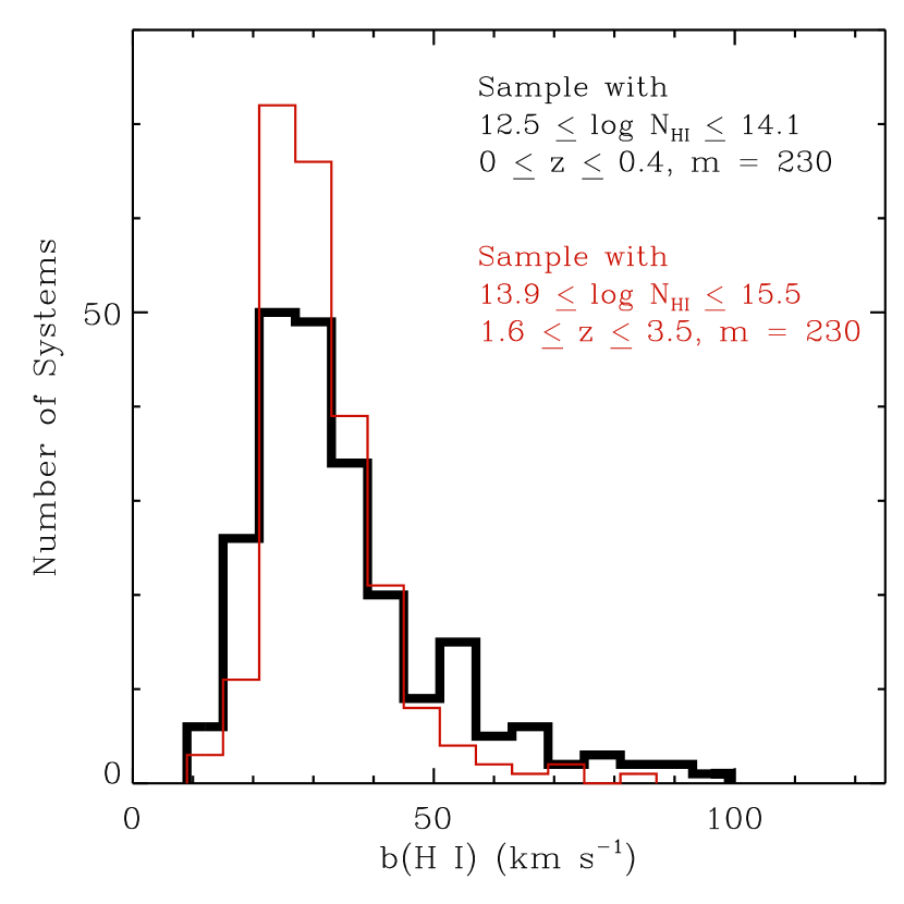
Figure 12.— Comparison of the distribution of $b$(H I) for the low $z$ STIS E140M sample of data points (black histogram) and for the high redshift sample (red histogram). The samples cover different ranges in $\log N_{\rm HI}$. Higher column density systems at high redshift are expected to be physically analogous to the low density systems at low redshift in an expanding universe. But note that in the high redshift sample, BLAs are often likely to be blends of narrower lines (see §4.2). The high redshift data are from Kim et al. (2002a). The number of absorbers in each sample is the same: $m=230$. Only data with less than 40% errors in $b$ and $N_{\rm HI}$ are considered in both samples.

4.4. Evolution of $d{\mathcal{N}}/dz$ as a Function of $b$

In Fig. 13, we show $d{\mathcal{N}}/dz$ ($0<b\leq 100$ ${\rm km\,s}^{-1}$), $d{\mathcal{N}}({\rm NLA})/dz$ ($b\leq 40$ ${\rm km\,s}^{-1}$), $d{\mathcal{N}}({\rm BLA})/dz$ ($40<b\leq 100$ ${\rm km\,s}^{-1}$), and $(d{\mathcal{N}}({\rm BLA})/dz)/(d{\mathcal{N}}({\rm NLA})/dz)$ as a function of the redshift. Only systems with $13.2\leq\log N_{\rm HI}\leq 14.0$ and $\sigma_{b}/b,\sigma_{N}/N\leq 0.4$ are considered in this figure. $d{\mathcal{N}}/dz$ was estimated for each sightline over the redshift interval available along a given sightline. The redshift at which $d{\mathcal{N}}/dz$ is plotted in Fig. 13 corresponds to the mean redshift interval in a given sightline. The vertical bars are Poissonian errors, while the horizontal bars represent the standard deviation around the mean of the observed redshifts of the Ly$\alpha$ absorbers. For the sample of Janknecht et al. (2006), several lines of sight have a redshift path larger than 0.6 and we divided those in two redshift intervals. The left diagram in Fig. 13 includes all the sightlines available in the various samples, while the right diagram includes all the sightlines available in the low $z$ sample and high $z$ samples of Kim et al. (2002a) and Kirkman & Tytler (1997), but only the highest quality data in the Janknecht et al. (2006) sample (see §4.2).

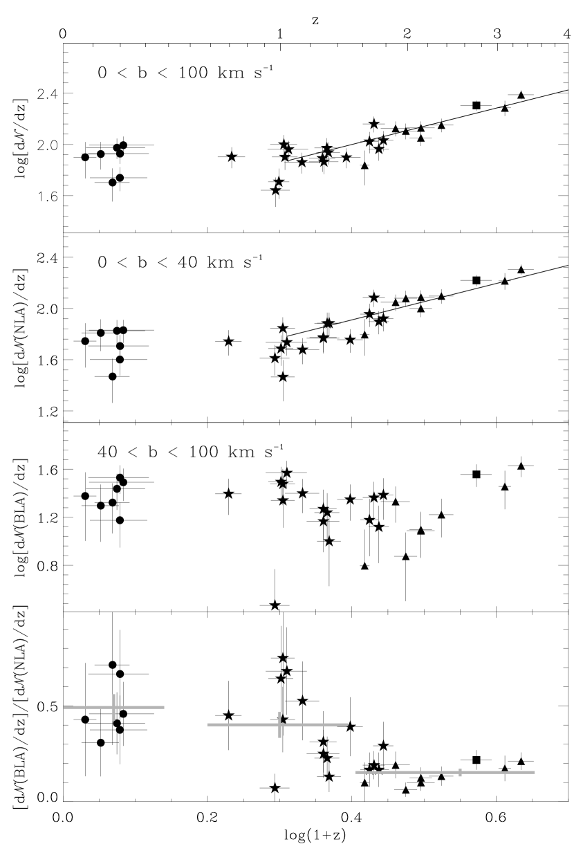
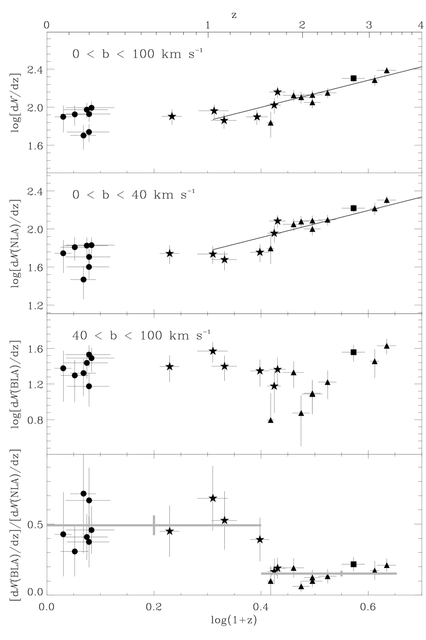
Figure 13.— The Ly$\alpha$ redshift density of the entire sample ($0<b\leq 100$ ${\rm km\,s}^{-1}$), the NLAs ($b<40$ ${\rm km\,s}^{-1}$), the BLAs ($40\leq b\leq 100$ ${\rm km\,s}^{-1}$), and the ratio of the Ly$\alpha$ redshift density fraction of the BLAs to the NLAs (bottom panel). We only consider absorbers with $13.2\leq\log N_{\rm HI}\leq 14.0$ and with errors less than 40% in $b$ and $N_{\rm HI}$. In the top two panels, the solid line shows $d{\mathcal{N}}/dz\propto(1+z)^{1.42}$ adopted from Kim et al. (2002a). The solid gray crosses in the bottom panels are the mean of $(d{\mathcal{N}}({\rm BLA})/dz)/(d{\mathcal{N}}({\rm NLA})/dz)$ where the horizontal bars indicate the redshift range over which the mean is estimated. The vertical bars are Poissonian errors. The symbols have the following meaning: data represented by circles are estimated from the low redshift sample (see Table 1 for the references); data represented by stars are estimated from the sample of Janknecht et al. (2006); data represented by triangles are estimated from the sample of Kim et al. (2002a); data represented by the square are estimated from the sample of Kirkman & Tytler (1997). The left panel considers all the data with the conditions listed above from these various samples, while in the right panel we remove the lowest quality measurements of Janknecht et al. (2006) (see §4.2).

The top two panels of Fig. 13 show the usual number density evolution with little or no evolution between redshifts 0 and $\sim$1.0–1.6, and an evolution of $d{\mathcal{N}}/dz$ with $z$ at higher redshift (see for example Kim et al. 2002a). At high redshift, $d{\mathcal{N}}/dz$ decreases with decreasing $z$ ($d{\mathcal{N}}/dz\propto(1+z)^{\gamma}$, $\gamma>0$) according to the expansion of the universe, which forces any initial baryon overdensity to thin out (e.g., Davé et al., 1999, and references therein). The expansion also results in a decrease of recombinations of the free electrons with the protons and thus in an additional decline in $d{\mathcal{N}}/dz$. The break in $d{\mathcal{N}}/dz$ near $z\sim 1.6$ ($\log(1+z)\sim 0.4$) is believed to be primarily caused by the drop in the UV background because of the declining quasar population (Theuns et al., 1998; Davé et al., 1999). In the top panels, the solid line shows $d{\mathcal{N}}/dz=(d{\mathcal{N}}/dz)_{0}(1+z)^{\gamma}$, where $\gamma=1.42$ was adopted from Kim et al. (2002a) who find this value for the weak absorbers with $13.1\leq\log N_{\rm HI}\leq 14.0$. The value of $(d{\mathcal{N}}/dz)_{0}$ was adjusted to match the data. For the entire sample ($0<b\leq 100$ ${\rm km\,s}^{-1}$) or the sample restricted to $b<40$ ${\rm km\,s}^{-1}$, this line represents well the evolution of $d{\mathcal{N}}/dz$ at $z>1$, but we note that when the best quality data are considered (right-hand side panel), the break in the evolution appears to occur at $z\sim 1.6$.

The second panels from the bottom in Fig. 13 show that $d{\mathcal{N}}({\rm BLA})/dz$ is generally similar or higher at low and mid redshift than between redshifts 1.6 and 2. At $z\gtrsim 2$, $d{\mathcal{N}}({\rm BLA})/dz$ increases and is larger at $z>2.5$ than $d{\mathcal{N}}({\rm BLA})/dz$ at $z<1.5$. The Hubble expansion must be the primary driver in the evolution of these structures at high redshift, and despite the expansion the BLA number density is comparable to $d{\mathcal{N}}({\rm BLA})/dz$ at high $z$, which contrasts remarkably from the evolution of $d{\mathcal{N}}({\rm NLA})/dz$ from low to high $z$. This difference is even more striking when we consider the ratio ${\mathcal{R}}\equiv(d{\mathcal{N}}({\rm BLA})/dz)/(d{\mathcal{N}}({\rm NLA})/dz)$ (bottom panels), which is higher in the low redshift sample than in the high redshift sample. On the left-hand side diagram, at mid redshift there is a very large scatter in the redshift range $0.9\lesssim z\lesssim 1.2$. This scatter clears up when only the best quality data of the mid-$z$ sample are considered (see right-hand side diagram). The distribution of ${\mathcal{R}}$ between redshifts $\sim$1.6 to 3.5 is actually nearly flat, showing that the slope controlling the evolution of $d{\mathcal{N}}({\rm NLA})/dz$ and $d{\mathcal{N}}({\rm BLA})/dz$ at $z\gtrsim 1.6$ must be about the same, further strengthening that NLAs and BLAs must follow a similar evolution dictated by the expansion of the universe. We note that ${\mathcal{R}}(z>2.5)$ is slightly larger than ${\mathcal{R}}(z\sim 2)$, possibly indicating some spurious increase of BLAs possibly due to line blending and blanketing effects that are more serious at $z>2.5$ than at $z\sim 2$. However, in the view of the large scatter in the various samples, this result does not appear statistically significant. The grey crosses in the bottom panels show the average ${\mathcal{R}}$ over the redshift range depicted by the horizontal grey bar (the vertical grey bar assumes Poissonian errors). At $z\lesssim 1.6$, ${\mathcal{R}}$ is larger than at $z>1.6$ as both the individual ${\mathcal{R}}$ and average ${\mathcal{R}}$ show. ${\mathcal{R}}$ is a factor 3.2 higher at $z\lesssim 0.4$ than at $z\gtrsim 1.6$. When only the best data of Janknecht et al. (2006) are considered, ${\mathcal{R}}$ at mid-redshift ($0.6\lesssim z\lesssim 1.5$) appears similar to the value observed at low redshift.

If we had considered systems with $b\leq 80$ ${\rm km\,s}^{-1}$, the same conclusions would be drawn. If we had considered a cutoff for the NLAs of $b=50$ or 60 ${\rm km\,s}^{-1}$ instead of 40 ${\rm km\,s}^{-1}$, similar conclusions would also be drawn. If absorbers with $13.2\leq\log N_{\rm HI}\leq 16.5$ are considered, we find that ${\mathcal{R}}(z<0.5)\sim 3{\mathcal{R}}(z>1.6)$, despite the fact many BLAs at high $z$ may actually be blends of narrower lines (see §4.2).

4.5. Implications

We find that (1) the distribution of $b$ for the BLAs has a distinctly more prominent high velocity tail at low and mid $z$ than at high $z$; (2) the median and mean $b$-values at low and mid $z$ are systematically higher than at high $z$; and (3) the ratio $(d{\mathcal{N}}({\rm BLA})/dz)/(d{\mathcal{N}}({\rm NLA})/dz)$ at low and mid $z$ is a factor $\sim$3 higher than at high $z$. These conclusions hold for a division $b=40$, 50, or 60 ${\rm km\,s}^{-1}$ between NLAs and BLAs. For the reasons discussed in §4.2, we believe that these are intrinsic properties of the evolution of the physical state of the gas that are not caused by comparing data with different S/N and line blending and blanketing effects. However, simulated spectra probing various $z$, with realistic inputs would certainly help to unravel how exactly some of these issues (e.g., continuum placement, line blending effect, different S/N ratios) balance each other. Our results strongly suggest that if the broadening is mostly thermal, a larger fraction of the low $z$ universe is hotter than the high $z$ universe, and if the broadening is mostly non-thermal, the low $z$ universe is more kinematically disturbed than the high $z$ universe. It is likely that both possibilities are true.

5. The Differential Column Density Distribution Function

The differential column density distribution $f(N_{\rm HI})$ is defined such that $f(N_{\rm HI},X)dXdN_{\rm HI}$ is the number of absorption systems with column density between $N_{\rm HI}$ and $N_{\rm HI}+dN_{\rm HI}$ and redshift path between $X$ and $X+dX$ (e.g., Tytler, 1987),

$$f(N_{\rm HI})dN_{\rm HI}dX=\frac{m}{\Delta N_{\rm HI}\Sigma\Delta X}dN_{\rm HI}dX\,,$$ (5)

where $m$ is the observed number of absorption systems in a column density range $\Delta N_{\rm HI}$ centered on $N_{\rm HI}$ obtained from our sample of 7 QSOs with a total absorption distance coverage $\Sigma\Delta X=2.404$ (see §2). Empirically, it has been shown that at low and high redshift, $f(N_{\rm HI})$ is well fitted by a single power law (e.g., Tytler, 1987; Petitjean et al., 1993; Hu et al., 1995; Lu et al., 1996; Kim et al., 2002a; Penton et al., 2000, 2004; Davé & Tripp, 2001):

$$f(N_{\rm HI})dN_{\rm HI}dX=C_{\rm HI}N_{\rm HI}^{-\beta}dN_{\rm HI}dX\,.$$ (6)

In Table 7, we show the results from the maximum-likelihood estimate of the parameters for the slope $\beta$ and the normalization constant where $C_{\rm HI}\equiv m_{\rm tot}(1-\beta)/[N^{1-\beta}_{\rm max}(1-(N_{\rm min}/N_{\rm max})^{1-\beta})]$ where $m_{\rm tot}$ is the total number of absorbers in the column density range $[N_{\rm min},N_{\rm max}]$. We separate our sample into absorbers with $b\leq 40$ ${\rm km\,s}^{-1}$ and $b\leq 150$ ${\rm km\,s}^{-1}$. For both $b$-samples we also choose three different column density ranges: (a) $[13.2,16.5]$ dex, (b) $[13.2,14.4]$ dex and (c) $[14.4,16.5]$ dex. The lower limit of sample (a) and (b) corresponds to our threshold of completeness. The largest observed column density in our sample is $\sim$$10^{16.5}$ cm^-2. Hence sample (a) corresponds to the whole sample with $W\gtrsim 90$ mÅ, while sample (b) only covers the weak Ly$\alpha$ systems, and (c) the strong Ly$\alpha$ systems. The cut at 14.4 was chosen because the sample analyzed by Penton et al. (2004) suggested a change of slope near this value (see below). Note that for each sample, we only consider absorbers with $\sigma_{b}/b\leq 0.4$ and $\sigma_{N}/N\leq 0.4$.

Figure 14.— The differential density distribution ($f(N_{\rm HI})$) without an incompleteness correction is plotted against $\log N_{\rm HI}$. Only H I absorbers with $b($H I$)\leq 40$ ${\rm km\,s}^{-1}$ and errors less than 40% in $b$ and $N_{\rm HI}$ are considered. The data are binned only for purpose of presentation. The solid line is a maximum-likelihood fit to the data ($f(N_{\rm HI})=C_{\rm HI}N_{\rm HI}^{-\beta}$) with the slope $\beta=1.76$ for H I column density systems between 13.2 and 16.5 dex. The dotted and dashed lines are maximum-likelihood fit to the data for $13.2\leq\log N_{\rm HI}\leq 14.4$ and $14.4\leq\log N_{\rm HI}\leq 16.5$, respectively (see Table 7 and §5 for more details).

In Fig. 14, we show the column density differential distribution of the identified absorbers for the combined sample with $b\leq 40$ ${\rm km\,s}^{-1}$ and the maximum-likelihood fits to the data. The fit to the sample with $b\leq 150$ ${\rm km\,s}^{-1}$ implies a general increase of $\beta$ (see Table 7) for the various column density intervals. For sample (a), if we vary $\log N_{\rm min}$ from 13.2 to 13.4, the results from the maximum-likelihood fit essentially do not change. If $\log N_{\rm min}<13.1$, $\beta$ decreases rapidly since our sample is not complete anymore. If $N_{\rm max}$ is reduced, $\beta$ will increase as sample (b) shows. For sample (b) with either $b\leq 40$ ${\rm km\,s}^{-1}$ or $b<150$ ${\rm km\,s}^{-1}$  if $\log N_{\rm min}$ increases by up to 0.4 and/or $\log N_{\rm max}$ varies by $\pm_{0.5}^{1.0}$ dex, the results do not statistically change. However, for sample (c), the results are more uncertain. While $\beta$ appears to flatten at larger column densities, there are too few absorbers with large H I column density to have a full understanding of the possible change in the slope. In particular, it is not clear from our sample where the break in the slope occurs since for $\log N_{\rm min}\approx 14.4\pm 0.5$ dex, $\beta$ is $\sim$1.5. At the 2$\sigma$ level, $\beta$ from sample (c) is essentially the same as for sample (a) and (b).

With GHRS and STIS grating moderate spectral resolution observations, Penton et al. (2004) found at $z\lesssim 0.1$ $\beta=1.65\pm 0.07$ for $12.3\leq\log N($H I$)\leq 14.5$ and $\beta=1.30\pm 0.30$ at $\log N($H I$)>14.5$ with few data points. In their work, $N$(H I) was obtained from the equivalent width assuming $b=25$ ${\rm km\,s}^{-1}$. Their results are consistent with the Key Project data presented by Weymann et al. (1998) and our results. Davé & Tripp (2001) derived $\beta=2.04\pm 0.23$ for $13\lesssim\log N($H I$)\lesssim 14$. They used STIS E140M spectra of two QSOs and were able to derive $b$ and $N$ independently using an automated Voigt profile fitting software but not allowing for BLAs. Within $1\sigma$, our results are the same.

At $z\gtrsim 1.5$, several studies using high resolution spectra obtained with the Keck and the VLT have shown that $\beta\approx 1.5$ for H I column density ranging from a few times $10^{12}$ cm^-2 up to a few times $10^{20}$ cm^-2 (e.g., Tytler, 1987; Hu et al., 1995; Lu et al., 1996), although there may be some deviation from a single power law at $\log N($H I$)>14$ (Petitjean et al., 1993; Kim et al., 1997, 2002a). There is also some suggestion that for a given H I interval, $\beta$ increases as $z$ decreases, but this is statistically uncertain at $z>2$ (Kim et al., 2002a). If we compare our results to Kim et al. (2002a), we find an increase of $\beta$ as $z$ decreases in the column density interval 13.2 to 14.4 dex or 13.2 to 16.5 dex, but not in the column density interval 14.4 to 16.5 dex, although in this range the number of data points is too small to draw any firm conclusion. Finally, the analysis of Janknecht et al. (2006) at $0.5<z<2.0$ shows that $\beta$ is intermediate between $\beta$ at $z<0.5$ and $\beta$ at $z>2$. Therefore, it appears that the column density distribution steepens with decreasing $z$ in the column density range 13.2 to 16.5 dex. A redshift dependence was found in the numerical results presented by Theuns et al. (1998), but the observed rate of evolution of $\beta$ appears to be smaller than their models suggest.

Table 7The Power Law Fit to the Distribution Function $f(N_{\rm HI})=C_{\rm HI}N_{\rm HI}^{-\beta}$

$[\log N_{\rm min},\log N_{\rm max}$]	$\beta$	$\log C_{\rm HI}$
$b\leq 40$ ${\rm km\,s}^{-1}$
$[13.2,16.5]$	$1.76\pm 0.06$	$12.1$
$[13.2,14.4]$	$1.83\pm 0.06$	$13.0$
$[14.4,16.5]$	$1.52\pm 0.10$	$8.4$
$b\leq 150$ ${\rm km\,s}^{-1}$
$[13.2,16.5]$	$1.84\pm 0.06$	$13.3$
$[13.2,14.4]$	$1.92\pm 0.05$	14.4
$[14.4,16.5]$	$1.61\pm 0.11$	9.9

Note. — Only data with $\sigma_{b}/b,\sigma_{N}/N\leq 0.4$ are included in the various samples (for more details, see §5).

6. The Baryon Density of the IGM

6.1. Narrow Ly$\alpha$ Absorption Lines

To estimate the baryon content of the photoionized Ly$\alpha$ forest at low $z$ we follow the method presented by Schaye (2001). The mean gas density relative to the critical density can be obtained from the H I density distribution function:

$$\Omega({\rm NLA})=\frac{\mu_{\rm H}m_{\rm H}H_{0}}{\rho_{c}\,c}\int N_{\rm HI}\frac{n_{\rm H}}{n_{\rm HI}}f(N_{\rm HI})dN_{\rm HI}$$ (7)

where $m_{\rm H}=1.673\times 10^{-24}$ g is the atomic mass of hydrogen, $\mu_{\rm H}=1.3$ corrects for the presence of helium, $H_{0}=100$ ${\rm km\,s}^{-1}$ Mpc^-1, $\rho_{c}=3H^{2}_{0}/(8\pi G)=1.06\times 10^{-29}$ g cm^-3 is the current critical density, $n_{\rm H}$ and $n_{\rm HI}$ the density of the total hydrogen and neutral hydrogen, respectively, $N_{\rm HI}$ the neutral hydrogen column density, and $f(N_{\rm HI})$ the differential density distribution function discussed in §5. Assuming that the gas is isothermal and photoionized, the previous equation can be simplified to,

$$\Omega({\rm NLA})\approx 2.2\times 10^{-9}h^{-1}\Gamma_{12}^{1/3}T_{4}^{0.59}\left(\frac{f_{g}}{0.16}\right)^{1/3}~{}~{}~{}~{}~{}~{}$$ (8)

$$\int_{N_{\rm min}}^{N_{\rm max}}N^{1/3}_{\rm HI}f(N_{\rm HI})dN_{\rm HI}$$

where $h\equiv H_{0}/(100$ ${\rm km\,s}^{-1}$ Mpc${}^{-1})$, $\Gamma_{12}$ is the H I photoionization rate in units of $10^{-12}$ s^-1, $T_{4}$ is the IGM temperature in units of $10^{4}$ K, and $f_{g}$ is the fraction of mass in gas in which stars and molecules do not contribute. Schaye (2001) states that in cold, collapsed clumps, $f_{g}\approx 1$, but on the scales of interest here $f_{g}$ is close to the ratio of the total baryon density to the matter density, which according to Spergel et al. (2003) is 0.16. We therefore set $f_{g}=0.16$. We use $\Gamma_{12}=0.05$ from Haardt & Madau (1996) for our average redshift $\bar{z}=0.19$. This value of $\Gamma_{12}$ is consistent with the value derived by Davé & Tripp (2001) at $\bar{z}=0.17$. The typical temperature of the IGM is not well defined in the current simulations of the low redshift universe. Schaye (2001) noted a good agreement between his estimate of $T_{4}$ and the Davé et al. (1999) estimate, we therefore use Eq. 3 for estimating $T_{4}$. But as these authors noted there is a very large scatter in the $T$–$\rho/\bar{\rho}$ relation at $z\sim 0$ producing uncertainty in the baryon determination from Eq. 8 because of temperature variations. Note for our calculation, we set $z=\bar{z}$. Because $\Omega({\rm NLA})\propto N^{4/3-\beta}_{\rm HI}$ with $\beta>4/3$, the low column density systems dominate $\Omega({\rm NLA})$, therefore we will set the temperature from $N_{\rm min}$ in Eq. 8. Furthermore since $N_{\rm min}$ dominates the solution of Eq. 8, using this equation is dependent on the data quality of the current sample. We therefore emphasize that we only derive the contributions of the denser parts of the photoionized Ly$\alpha$ forest.

To estimate the baryon content of the photoionized regions, we only use H I absorbers with $b\leq 40$ ${\rm km\,s}^{-1}$. Broader systems are here assumed to be principally collisionally ionized. For the interval of H I column density $10^{13.2}$–$10^{16.5}$ cm^-2, using the best fit parameters of $f(N_{\rm HI})$ listed in Table 7 for this range of column densities and with $(\Gamma_{12},T_{4},f_{g},h)=(0.05,1.2,0.16,0.7)$, we find $\Omega({\rm NLA})/\Omega_{\rm b}\simeq 0.19$ for absorbers with $\log N_{\rm HI}\geq 13.2$, where $\Omega_{\rm b}=0.044$ is the ratio of the total baryon density to the critical density (Spergel et al., 2003; Burles et al., 2001; O’Meara et al., 2001). If we assume that the power law described in §5 fits the data extending to the lower observed column density (12.42 dex), we find $\Omega({\rm NLA})/\Omega_{\rm b}=0.29$ for the column density range $[12.4,16.5]$ with $(\Gamma_{12},T_{4},f_{g},h)=(0.05,0.6,0.16,0.7)$. Such an assumption is not unrealistic since, in high redshift spectra, Lu et al. (1996) and Kirkman & Tytler (1997) show using their simulation results that weak absorbers (down to 12.1–12.5 dex) follow the same column density distribution as the stronger absorbers. Assuming $\beta=1.76$ (see Table 7) and Eq. 3, the dependence between $\Omega({\rm NLA})/\Omega_{\rm b}$ and $N_{\rm min}$ can be approximated by $\Omega({\rm NLA})/\Omega_{\rm b}\simeq 0.2\,(N_{\rm min}/[10^{13.2}\,{\rm cm}^{-2}])^{-0.18}$.

With the available data, there is no indication of subcomponent structure in the broad Ly$\alpha$ absorption lines. However, broadening mechanisms other than thermal may also be important. If this is the case, the thermal broadening could decrease significantly for the broad Ly$\alpha$ absorption lines, implying that many of those lines would arise in the photoionized IGM, not the WHIM. If the complete sample with $\log N_{\rm HI}=[13.2,16.5]$ and $b\leq 150$ ${\rm km\,s}^{-1}$ is considered, $\Omega(b<150{\mbox{${\rm km\,s}^{-1}$}})/\Omega_{\rm b}\gtrsim 0.23$ for $(\Gamma_{12},T_{4},f_{g},h)=(0.05,1.2,0.16,0.7)$. If the sample with $\log N_{\rm HI}=[12.4,16.5]$ and $b\leq 150$ ${\rm km\,s}^{-1}$ is considered, $\Omega(b<150{\mbox{${\rm km\,s}^{-1}$}})/\Omega_{\rm b}=0.40$ for $(\Gamma_{12},T_{4},f_{g},h)=(0.05,0.6,0.16,0.7)$. Therefore, if the BLAs are tracing photoionized gas, the estimate of $\Omega$ would increase by a factor $\sim$1.3. These BLAs would not then contribute to the baryon budget in the BLAs determined in §6.2.

To estimate a reliable error on $\Omega({\rm NLA})$ remains a difficult task with our current knowledge. The estimate of $\Omega({\rm NLA})$ is model dependent since the representative temperature of the IGM is not well known. More numerical simulations of the low redshift IGM spanning a wider range of parameters and using the results from the current sample may tighten $\Gamma$ and $T$. If $T$ changes by 20%, $\Omega({\rm NLA})/\Omega_{\rm b}$ can change by about 10–15%; if $\Gamma$ changes by 20%, $\Omega({\rm NLA})/\Omega_{\rm b}$ can change by about 10%. The $\Omega$ estimate is also very sensitive to the slope $\beta$: a change of $\beta$ by $\pm 0.005$ can introduce a change in $\Omega({\rm NLA})/\Omega_{\rm b}$ by about $\mp 4$%. Furthermore the low column density absorbers dominate the baryon fraction and the low column density cutoff, $N_{\rm min}$, is unknown. Therefore, while the exact baryon content is uncertain in the photoionized IGM, it is clear that the photoionized Ly$\alpha$ forest is a large reservoir of baryons. The baryon fraction in the diffuse photoionized phase traced by (narrow) Ly$\alpha$ absorbers predicted by cosmological models in the low redshift universe varies by a factor 2 ($\sim$20–40%) among the various simulations (Davé et al., 2001), in general agreement with our results. We note that Penton et al. (2004) derived $\Omega({\rm Ly\alpha})/\Omega_{\rm b}=0.29\pm 0.04$ for the photoionized phase in the column density range [12.5,17.5] dex. In view of our discussion on the various uncertainties, we believe that their error estimate appears optimistic.

6.2. Broad Ly$\alpha$ Absorption Lines

Baryons also reside in the WHIM, a shock-heated intergalactic gas with temperatures in the range 10⁵ to 10⁷ K. Cosmological hydrodynamical simulations predict that the WHIM may contain 30–50% of the baryons at low redshift (Cen & Ostriker 1999; Davé et al. 1999). BLAs may trace the 10⁵ to 10⁶ K WHIM if the broadening is purely thermal, following $T[{\rm K}]=(b[{\rm km\,s^{-1}}]/0.129)^{2}$. The cosmological mass density of the broad Ly$\alpha$ absorbers in terms of today critical density can be written (Richter et al., 2004; Sembach et al., 2004) as,

$$\Omega({\rm BLA})=\frac{\mu_{\rm H}m_{\rm H}H_{0}}{\rho_{c}\,c}\frac{\Sigma f_{\rm H}(T_{i})N_{\rm HI}(i)}{\Sigma\Delta X}$$

$$\Omega({\rm BLA})\approx 1.667\times 10^{-23}\frac{\Sigma f_{\rm H}(T_{i})N_{\rm HI}(i)}{\Sigma\Delta X}$$ (9)

where $f_{\rm H}(T)$ being the conversion factor between H I and total H and the other symbols have the same meaning as in Eq. 7. For our sample, $\Sigma\Delta X=2.404$. In Eq. 9 the sum of $f_{\rm H}(T_{i})N_{\rm HI}(i)$ over index $i$ is a measure of the total hydrogen column density in the BLAs. When collisional ionization equilibrium (CIE) is assumed, the conversion factor between H I and total H was approximated by Richter et al. (2004) from the values given in Sutherland & Dopita (1993) for temperatures $10^{5}-10^{6}$ K:

$$\log f_{\rm H}(T)\approx-13.9+5.4\log T-0.33(\log T)^{2}\,.$$ (10)

For low-density absorbers, the CIE hypothesis is, however, probably a poor approximation because the photoionization from the UV background is important (Richter et al., 2006b). Recently, Richter et al. (2006a) used the output of the numerical simulation, carried out by Fang & Bryan (2001) to investigate the intervening O VI absorption in the WHIM, to study the BLAs in the low redshift IGM. They found that a significant number of BLAs could be photoionized, in particular systems that have relatively low $b$-values in the range 40–65 ${\rm km\,s}^{-1}$. Their simulation that includes collisional ionization and photoionization suggests that the hydrogen ionization fraction can be approximated as:

$$\log f_{\rm H}(T)\approx-0.75+1.25\log T\,.$$ (11)

According to Fig. 5 in Richter et al. (2006a), the CIE hypothesis (Eq. 10) provides a firm lower limit to $f_{\rm H}(T)$. Eqs. 10 and 11 converge as $b$ increases, but never intersect.

In Table 5 and §3.3, we saw that the S/N has little effect on the estimate for $d{\mathcal{N}}({\rm BLA})/dz$ for the highest S/N spectra, but can reduce $d{\mathcal{N}}({\rm BLA})/dz$ for the lowest S/N data in our sample. To reduce the uncertainty from the broadening of the H I absorbers found in low S/N spectra, we restricted our sample to absorbers with $\sigma_{b}/b,\sigma_{N}/N\leq 0.3$. To estimate $\Omega({\rm BLA})$, we consider the following $b$-value intervals: $[40,150]$, $[40,65]$, and $[65,150]$ ${\rm km\,s}^{-1}$. In the $[40,65]$ ${\rm km\,s}^{-1}$ interval, Richter et al. (2006a) found that about a $1/3$ of the BLAs traces cool photoionized gas ($T<2\times 10^{4}$ K), i.e. $b_{\rm nt}\gg b_{\rm th}$ for these systems. If all the BLAs are assumed to be thermally broadened, we would overestimate $\Omega({\rm BLA})$. We therefore randomly pick 2/3 of the BLAs in the $[40,65]$ ${\rm km\,s}^{-1}$  $b$-range to estimate $f_{\rm H}$. (We note that the baryon content of the photoionized BLAs with $T\lesssim 10^{4}$ K is less than 1–2% according to Richter et al. 2006a.) In the $[65,150]$ ${\rm km\,s}^{-1}$ $b$-range, the number of BLAs tracing cool photoionized systems is small (less than $\sim$5%) and we assume that all the BLAs in this range of $b$-values are mostly thermally broadened. With the conditions listed above, there are 12 systems in the $[65,150]$ ${\rm km\,s}^{-1}$ interval and 31 in the $[40,65]$ ${\rm km\,s}^{-1}$ $b$-range. In Table 8, we summarize our estimates of $\Omega({\rm BLA})/\Omega_{\rm b}$ using Eqs. 9, 10, and 11 where $T$ was derived assuming $b_{\rm th}\approx 0.9b_{\rm obs}$ following the simulation of Richter et al. (2006a). The largest difference in the estimates of the baryon budget from CIE and Richter et al.’s model is for low $b$-values, where photoionization plays a more important role. We note that that if we restricted our sample to systems with $\sigma_{b}/b,\sigma_{N}/N\leq 0.2$, $\Omega({\rm BLA})/\Omega_{\rm b}$ would decrease by a factor $\sim$1.2, but would increase by a factor $\sim$1.2–2.4 if $\sigma_{b}/b,\sigma_{N}/N\leq 0.4$.

As for the estimate of the baryon budget of the NLAs, with our current knowledge it appears a very difficult task to estimate an error on the baryon budget in BLAs. It is model dependent. Richter et al. (2006a) provided estimates of the amount of the BLAs that probe cool photoionized gas and the amount of thermal broadening in BLAs. These estimates may change with refined cosmological models. If we assume that the broadening for all the BLAs is purely thermal ($b_{\rm th}=b_{\rm obs}$), the estimates of $\Omega({\rm BLA})/\Omega_{\rm b}$ in the $[40,150]$ ${\rm km\,s}^{-1}$ $b$-range would increase by a factor 1.6, i.e. in the CIE model, $\Omega({\rm BLA})/\Omega_{\rm b}\simeq 0.13$, and in the collisional ionization plus photoionization model of Richter et al. (2006a), $\Omega({\rm BLA})/\Omega_{\rm b}\simeq 0.32$. The broadening could be due to several unresolved components in some cases or the non-thermal broadening could be important. This is partly accounted for since we remove a 1/3 of the BLAs in the $[40,65]$ ${\rm km\,s}^{-1}$ $b$-range. Since we discarded systems with large errors in $b$ and $N$, for the current data set, a single Gaussian fit provides a good representation of the observed profiles. However, as we discussed in §3.2, the formal errors given by the fit may not be sufficient especially for the weaker and broader systems. Richter et al. (2006b) and the other papers mentioned in Table 1 present several examples of BLAs that are well fitted with a single Gaussian with sometimes the presence of several H I Lyman series transitions that further constrain the fit parameters (see also the discussion in §4.2). To further explore the quality of the profile fitting, the Cosmic Origin Spectrograph (COS) could really improve the situation by increasing the number of sightlines and increasing the S/N in the spectra. Additional theoretical simulations of the low-$z$ IGM with higher resolution and refined physics combined with the analysis of simulated spectra should improve our understanding of the BLAs.

Table 8Estimates of the Baryon Density in BLAs

$b$ [${\rm km\,s}^{-1}$]	$\frac{\Omega_{\rm CIE}({\rm BLA)}^{a}}{\Omega_{\rm b}}$	$\frac{\Omega_{\rm C+P}({\rm BLA)}^{b}}{\Omega_{\rm b}}$
$[40,65]$	0.03	0.11
$[65,150]$	0.05	0.09
$[40,150]$	0.08	0.20

Note. — Only data with $\sigma_{b}/b,\sigma_{N}/N\leq 0.3$ and $\log N_{\rm HI}\geq 13.2$ are included in the various samples. In the $[40,65]$ ${\rm km\,s}^{-1}$ interval, only 2/3 of the BLAs are considered. We derive the temperature of the absorbers assuming $b_{\rm th}=0.9b_{\rm obs}$. The baryon density in the interval $[40,150]$ ${\rm km\,s}^{-1}$ is the sum of $\Omega($BLA) in the two other intervals. $a$: Obtained from Eqs. 9 and 10; baryonic density for the BLAs assuming that they are collisionally ionized and CIE applies. $b$: Obtained from Eqs. 9 and 11; baryonic density for BLAs assuming that they are collisionally ionized and photoionized using the results from the hydrodynamical simulations of Richter et al. (2006a) (see §6.2 for more details). $\Omega_{\rm b}=0.044$ (Spergel et al., 2003).

In summary, the CIE estimate provides a firm and conservative limit for the baryon budget in collisionally ionized BLAs, $\Omega({\rm BLA)}/\Omega_{\rm b}\gtrsim 0.1$ for systems with $40<b\lesssim 150$ ${\rm km\,s}^{-1}$, $\log N_{\rm HI}\geq 13.2$, $\sigma_{b}/b,\sigma_{N}/N\leq 0.3$. The BLA simulations show that the ionization fraction in BLAs is governed by collisional ionization and photoionization. Therefore, $\Omega({\rm BLA)}/\Omega_{\rm b}\gtrsim 0.2$ (with the same constraints that those listed above) should reflect better the baryon budget of the BLAs in the low-$z$ IGM. This is likely a lower estimate as well since the existing observations do not have the S/N to detect the broader systems (where most of the baryons are believed to exist) and the numerous weaker BLAs (see Fig. 6), and are not complete at $b\gtrsim 80$ ${\rm km\,s}^{-1}$.

6.3. Baryon Budget of the Low Redshift Universe

At redshift 2–4, observations of the Ly$\alpha$ forest show that about 80–90% of the total baryon budget is found in the cool photoionized phase of IGM (Rauch et al., 1997; Weinberg et al., 1997; Kim et al., 2001). In the low redshift universe, Fukugita et al. (1998) show that 9–10 % of the total baryons are found in galaxies (stars, neutral gas, molecular gas) and $\sim$6 % of the baryons are associated with the hot plasma in clusters of galaxies.

Our analysis of the low redshift Ly$\alpha$ forest shows the presence of NLAs and BLAs. The NLAs trace the cool photoionized IGM, while the BLAs are likely to probe the cool photoionized IGM and the hot highly-ionized gas in the WHIM. There are still many uncertainties that are not controlled in the determination of the baryon content in the low redshift Ly$\alpha$ forest. But at least 20% of the baryons are found in the denser parts of the photoionized phase (NLAs, $b\leq 40$ ${\rm km\,s}^{-1}$, $\log N_{\rm HI}\geq 13.2$, and $\sigma_{b}/b,\sigma_{N}/N\leq 0.4$) and at least $\sim$10% are found in the WHIM (BLAs, $40<b\leq 150$ ${\rm km\,s}^{-1}$, $\log N_{\rm HI}\geq 13.2$, $\sigma_{b}/b,\sigma_{N}/N\leq 0.3$), corresponding to at least 30% of the total baryon budget. We believe that these limits are very conservative since they do not take into account the low column density photoionized absorbers and the broadest BLAs. Furthermore recent simulations of the BLAs in low redshift universe show that the BLAs may trace both photoionized and collisionally ionized gas. Using the simulations of Richter et al. (2006a), we find that the BLAs include at least 20% of the baryons. We have also seen that $\Omega$ in the cool photoionized IGM is dominated by the low column density H I absorbers (i.e. absorbing gas with overdensity $\rho/\bar{\rho}\lesssim 2$). If the weak systems follow the same differential column density distribution function as the stronger absorbers, the cool photoionized gas traced by the NLAs with $\log N_{\rm HI}\geq 12.4$ can contain $\sim$30% of the total baryons. Combining these NLA and BLA budgets, the low redshift IGM contains at least $\sim$50% of the baryons. This is much larger than the known amount of baryons in galaxies and clusters of galaxies in the low redshift universe. High S/N data will allow us to search for the weakest Ly$\alpha$ absorbers ($\lesssim 10^{12.5}$ cm^-2) and estimate their column density distribution, search for the very broad absorbers and the weak BLAs, and provide a better understanding of their physical nature. It is, however, already apparent from this study that the IGM traced by the narrow and broad Ly$\alpha$ absorption lines in the low redshift universe is a major reservoir of baryons.

7. Summary

We analyze the physical properties of the low-$z$ IGM traced by H I absorbers from a sample of 7 QSOs observed with the E140M mode of STIS ($R\sim 44000$) and with FUSE ($R\sim 15000$). These seven lines of sight were fully analyzed and presented in recent and future papers (see references in Table 1 and the Appendix of this paper). Our sample has a total unblocked redshift path of 2.064 corresponding to a total absorption distance of 2.404 and is complete for $\log N_{\rm HI}\gtrsim 13.2$ provided $b\lesssim 80$ ${\rm km\,s}^{-1}$. With high spectral resolution the column density ($N_{\rm HI}$) and the Doppler parameter ($b$) were independently estimated, providing the opportunity to directly study the distribution and evolution of $b$. The spectral resolution of the STIS E140M H I observations in our sample is similar to that of the high redshift ($z\gtrsim 1.5$) observations obtained with Keck/HIRES and VLT/UVES. This similarity allows a relatively simple study of the evolution of the $b$-parameter of the neutral hydrogen gas in the intergalactic medium. Because the nominal lower temperature of the WHIM is $T\sim 10^{5}$ K, we consider two different populations of H I absorbers throughout this work: narrow Ly$\alpha$ absorbers (NLAs) have $b\leq 40$ ${\rm km\,s}^{-1}$ and the broad Ly$\alpha$ absorbers (BLAs) have $b>40$ ${\rm km\,s}^{-1}$. Our main findings applicable at redshifts $z\lesssim 0.4$ are summarized as follows:

1. The H I Doppler width distribution has a high velocity tail that develops at $b\approx 40$–60 ${\rm km\,s}^{-1}$. The $b$–$N_{\rm HI}$ distribution reveals for the NLAs an increase of $b$ with increasing $N_{\rm HI}$ with a very large scatter. We find that most of the BLAs are found in the H I column density range [13.2,14.0] dex and the broader systems are found for $13.1\lesssim\log N_{\rm HI}\lesssim 13.5$. Recent cosmological simulations of BLAs show a good agreement with the observations, but clearly indicate that broader absorbers and many weak BLAs ($\log N_{\rm HI}\lesssim 13.1$) remain to be discovered.

2. We find $d{\mathcal{N}}({\rm BLA})/dz=30\pm 4$ for absorbers with $40<b\lesssim 150$ ${\rm km\,s}^{-1}$, $\log N_{\rm HI}\geq 13.2$, and $\sigma_{b}/b,\sigma_{N}/N\leq 0.4$. The narrow H I absorbers are more frequent, with $d{\mathcal{N}}({\rm NLA})/dz=66\pm 6$ for absorbers with $b\leq 40$ ${\rm km\,s}^{-1}$, $\log N_{\rm HI}\geq 13.2$, and $\sigma_{b}/b,\sigma_{N}/N\leq 0.4$. Very narrow absorbers ($b\lesssim 15$ ${\rm km\,s}^{-1}$) with $\log N_{\rm HI}\geq 13.2$ are scarce. The number of weak NLAs and BLAs ($\log N_{\rm HI}\leq 14$) is far larger than the number of strong NLAs and BLAs, respectively.

3. For the narrow absorbers with $13.2\leq\log N_{\rm HI}\leq 16.5$ and $\sigma_{b}/b,\sigma_{N}/N\leq 0.4$, we find that the column density distribution, $f(N_{\rm HI})\propto N^{-\beta}_{\rm HI}$, can be fitted with $\beta=1.76\pm 0.06$. For the entire sample (i.e. including NLAs and BLAs), the slope changes to 1.84 for the same column density range. We confirm an increase of $\beta$ with decreasing $z$ when our results are compared to higher redshift analyses. There is some weak evidence for a break at $\log N_{\rm HI}\sim 14.4$, but the location of this break is uncertain because of the small number statistics for the higher column density lines.

4. We argue that various samples probing different redshift ranges can be directly compared when the conditions $0<b\leq 100$ ${\rm km\,s}^{-1}$, $13.2\leq\log N_{\rm HI}\leq 14.0$, and $\sigma_{b}/b,\sigma_{N}/N\leq 0.4$ are set. The distribution of $b$ for the broad absorbers has a distinctly more prominent high velocity tail at low $z$ than at high $z$ ($1.5\lesssim z\lesssim 3.6$). The median and mean $b$-values are systematically larger by $\sim$15–30% at $z\lesssim 0.5$ than at $1.5\lesssim z\lesssim 3.6$. The ratio of the number density of BLAs to NLAs at low $z$ is larger than at high $z$ by a factor $\sim$3. This suggests that a larger fraction of the low-$z$ universe is hotter than at $1.5\lesssim z\lesssim 3.6$ and/or the low-$z$ universe is more kinematically disturbed than the high-$z$ universe.

5. The NLAs trace the cool photoionized IGM at $T\lesssim 10^{4}$ K, and we find that $\Omega({\rm NLA})/\Omega_{\rm b}\simeq 0.2\,(N_{\rm min}/[10^{13.2}\,{\rm cm}^{-2}])^{-0.18}$ (when $f(N_{\rm HI})\propto N^{-1.76}_{\rm HI}$ and assuming $N_{\rm HI}\propto T^{-0.42}$), where $N_{\rm min}$ is the lowest H I column density in the sample considered to estimate $\Omega({\rm NLA})$. The contribution to the baryon budget of the denser parts of the photoionized Ly$\alpha$ forest with $\log N_{\rm HI}\gtrsim 13.2$ is $\sim$20%. If the weakest H I absorber with $\log N_{\rm HI}=12.4$ follows the same $f(N_{\rm HI})$, the cool photoionized gas with $\log N_{\rm HI}\gtrsim 12.4$ contains about 30% of the total baryons.

6. The BLAs trace mostly the highly-ionized gas in the WHIM at $T\simeq 10^{5}$–$10^{6}$ K if the width of the BLAs is dominated by thermal motions. The assumption of collisional ionization equilibrium provides a firm lower limit to the amount of the baryons in the WHIM traced by the BLAs ($40<b\lesssim 150$ ${\rm km\,s}^{-1}$, $\log N_{\rm HI}\geq 13.2$, $\sigma_{b}/b,\sigma_{N}/N\leq 0.3$): $\Omega({\rm BLA})/\Omega_{\rm b}\gtrsim 10$%. If a hydrodynamical simulation including the effects of collisional ionization and photoionization is used to estimate the ionization correction for the BLAs, we find that at least 20% of the baryons are in the BLAs.

7. Our most conservative estimate of the baryon budget in absorbers with $\log N_{\rm HI}\gtrsim 13.2$ shows that the Ly$\alpha$ forest has at least about 30% of the baryons (NLAs+BLAs), far larger than the baryon budget in galaxies. We suggest that the low redshift IGM with $T\lesssim 10^{6}$ K traced by the NLAs with $\log N_{\rm HI}\gtrsim 12.4$ and the BLAs with $\log N_{\rm HI}\gtrsim 13.2$ could contain at least 50% of the baryons (this is a lower limit since the broader BLAs where most the baryons reside remain to be discovered). The estimates of the amount of baryons still rely, however, on critical assumptions (e.g. pure thermal broadening versus other broadening mechanisms, temperature of the IGM, behavior of the weak narrow systems) that produce uncertainties that are currently not well controlled. Observationally, if COS is deployed, our understanding of the BLAs, in particular, will improve given the high S/N spectra that COS should obtain (but with approximately 2 times lower resolution than for the STIS observations presented here). The present paper and future observations of the low-$z$ IGM should motivate more precise cosmological simulations of the low- and high-$z$ IGM that are needed for our understanding of the intrinsic properties of the BLAs and NLAs.

We have revisited the H I measurements presented by Williger et al. (2006) toward PKS 0405–123. We were first motivated to produce a new analysis of the PKS 0405–123 FUSE and STIS/E140M spectra because Williger et al. (2006) noted that several of their BLAs may be noise features. For our work, we needed to clearly differentiate a real detection from a noise feature. While reanalyzing the BLAs, we noted that some narrow H I lines were either not present in the spectra at the 3$\sigma$ level (although Williger et al. claimed to report only 4$\sigma$ features) or were misidentified. We have not identified the ultimate origin of the problem, but we suspect that the difference with Williger et al. can ultimately be traced to a difference in the manner in which the continuum placement was done. Williger et al. fitted a single global continuum, while we determine continua separately placed within $\pm$1000–3000 ${\rm km\,s}^{-1}$ of each absorption line. We therefore produce here a new line list and new measurements for H I toward PKS 0405-0123 in Table A1. This reanalysis also provides an overall coherent data sample, since the other sightlines were analyzed following the same methodology. In Table A1, we report our measurements for H I toward PKS 0405–123. These H I absorbers are detected at least at the 3$\sigma$ level. We list in this table the observed wavelengths and the rest-frame equivalent widths of the Ly$\alpha$ transition. The listed column densities and Doppler parameters were measured in the rest-frame by N. Lehner (NL) following the method described in Lehner et al. (2006). The weak absorbers ($\log N_{\rm HI}<14$) were also independently measured by P. Richter (PR) using the method described in Richter et al. (2004). In particular, different profile fitting software was used by NL and PR. In Fig. 15, we compare the column densities and $b$-values (for the weak absorbers) presented by Williger et al. (2006) to those listed in Table A1 (left panels). On the right-hand side, we present the measurements obtained by PR against those listed in Table A1. For both $b$ and $N_{\rm HI}$, there is an excellent agreement between PR and NL measurements at the 1$\sigma$ level. In contrast, Williger et al. (GW) found generally larger column densities and Doppler parameters. The main difference between our analysis (NL and PR) and GW’s analysis is that we systematically and independently chose the continua within $\pm 1000$–3000 ${\rm km\,s}^{-1}$ of the H I absorption line, while GW fitted the continuum using a semi-automatic procedure (AUTOVP) combined with custom fitting in the vicinity of the QSO emission lines. Since these weak absorbers are generally detected solely in Ly$\alpha$, the continuum placement is critical. Our method for the continuum placement was followed for all the other sightlines presented in this work. For the absorbers where Ly$\alpha$ and Ly$\beta$ are detected, our measurements and those made by GW agree within 1$\sigma$.

Absorbers with $\log N_{\rm HI}>14$ are detected in several Lyman series lines. For the absorbers that were fitted with a single component ($z=0.03000,0.35099,0.40571,0.40886$), GW and our measurements are in agreement within 1$\sigma$. GW fitted the systems listed in Table A1 at $z=(0.09657,0.09659)$ and (0.18262,0.18287) with a single component. We found that a 2-component fit provides a statistically better fit. The total column densities for those absorbers are in agreement within 1$\sigma$ with those measured by GW. For the partial Lyman limit system at $z=0.167$, we found that 5 components provide a better fit to this complicated absorber (see Fig. 16 and note (6) in Table A1). We note that our fit is not yet as good as it should be despite our best effort (see Fig. 16). In particular, the broad component at $z=0.16678$ may actually be narrower since metals-ions such as C III are detected at this redshift (this directly affects the measurements of the absorber at $z=0.16661$ where C III is also detected). Finally, we fitted the system at $z=0.36808$ with 4 components. This is not statistically different from the 2 component fit presented by GW, but the 4-component fit appears to be a better model when the kinematics of the metal-ions are taken into account (see note (12) in Table A1 for more details).

In Table A2, we report the list of features that were identified as Ly$\alpha$ and claimed to be detected at least at the 4$\sigma$ level by GW. These features are actually either non-detections at the 3$\sigma$ level (according to our measurements) or were misidentified. The 181 Ly$\alpha$ absorbers toward PKS 0405–123 reported by GW now reduce to 74 absorbers (and in a few cases, those are multi-component absorbers).

Table 9IGM H I revised measurements toward PKS 0405–123^a

$\lambda$	$z$	$W_{\rm Ly\alpha}$	$\log N_{\rm HI}$	$b_{\rm HI}$	Note
(Å)		(mÅ)	(dex)	(${\rm km\,s}^{-1}$)
1230.1364	0.01190	$53.5\pm 11.5$	$13.09\pm 0.09$	$7.2\pm 3.0$
1233.8078	0.01492	$35.1\pm 10.9$	$13.09\pm 0.11$	$11.5\pm 5.9$
1236.1053	0.01681	$45.3\pm 14.1$	$13.08\pm 0.10$	$25.0\pm 11.0$
1240.3360	0.02029	$48.7\pm 14.1$	$13.12\pm 0.12$	$32.2\pm 15.5$
1251.9578	0.02985	$65.4\pm 9.6$	$13.36\pm 0.13$	$12.4:$
1252.1401	0.03000	$255.4\pm 16.6$	$14.37\pm 0.04$	$20.3\pm 0.9$
1254.5228	0.03196	$90.5\pm 19.2$	$13.33\pm 0.08$	$54.0\pm 16.1:$
1272.3689	0.04664	$51.4\pm 12.1$	$13.09\pm 0.09$	$27.7\pm 9.2$
1287.3459	0.05896	$41.0\pm 10.2:$	$13.34\pm 0.10$	$76.5\pm 26.8$	1
1287.6984	0.05925	$48.3\pm 9.3$	$12.76\pm 0.18$	$10.8:$	1
1303.4171	0.07218	$49.5\pm 10.8$	$13.09\pm 0.08$	$44.8\pm 14.4$
1303.8182	0.07251	$44.6\pm 9.6$	$13.06\pm 0.07$	$19.0\pm 5.1$
1306.2252	0.07449	$31.8\pm 8.7$	$12.85\pm 0.11$	$17.5\pm 9.0$
1307.1249	0.07523	$42.1\pm 11.6$	$13.05\pm 0.11$	$47.7\pm 20.3$
1314.6134	0.08139	$236.0\pm 18.7$	$13.79\pm 0.02$	$54.3\pm 3.5$
1327.3172	0.09184	$472.2\pm 24.4$	$14.60\pm 0.02$	$39.1\pm 0.9$	2
1333.0673	0.09657	$487.2\pm 27.9$	$14.57\pm 0.04$	$30.3\pm 2.3$	3
1333.0916	0.09659	$\cdots$	$13.90\pm 0.18$	$69.8\pm 19.8$	3
1333.7845	0.09716	$50.9\pm 6.7$	$13.02\pm 0.05:$	$29.0\pm 3.2$
1340.8597	0.10298	$96.3\pm 19.2$	$13.40\pm 0.07$	$86.6\pm 19.4$
1374.9470	0.13102	$108.9\pm 15.1$	$13.46\pm 0.05$	$51.9\pm 7.9$
1376.5395	0.13233	$142.5\pm 13.5$	$13.64\pm 0.03$	$22.3\pm 1.7$
1377.4270	0.13306	$72.9\pm 11.5$	$13.29\pm 0.06$	$31.7\pm 6.3$
1378.2902	0.13377	$90.3\pm 16.2$	$13.34\pm 0.06$	$42.8\pm 8.1$
1381.5604	0.13646	$76.8\pm 13.2$	$13.34\pm 0.06$	$53.8\pm 10.8$	4
1399.6739	0.15136	$49.2\pm 10.4$	$13.20\pm 0.07$	$37.0\pm 8.8$
1400.7436	0.15224	$114.8\pm 13.2$	$13.54\pm 0.04$	$22.4\pm 2.1$
1401.7162	0.15304	$223.3\pm 16.8$	$13.80\pm 0.03$	$46.3\pm 3.4$
1411.6482	0.16121	$157.5:\pm 16.1$	$13.71\pm 0.04$	$54.1\pm 7.7$	5
1412.0007	0.16150	$120.7:\pm 13.1$	$13.27\pm 0.09$	$18.2\pm 4.4$	5
1413.8485	0.16302	$110.7\pm 16.5$	$13.42\pm 0.05$	$34.0\pm 5.2$
1418.2128	0.16661	$\cdots$	$13.29\pm 0.08:$	$7.9\pm 2.1:$	6
1418.4194	0.16678	$\cdots$	$13.91\pm 0.04:$	$74.9\pm 7.2:$	6
1418.6139	0.16694	$\cdots$	$15.33\pm 0.20$	$13.5\pm 3.7$	6
1418.8327	0.16712	$\cdots$	$16.30\pm 0.09$	$12.5\pm 5.6$	6
1418.8571	0.16714	$844.0\pm 41.6$	$16.27\pm 0.13$	$29.9\pm 1.2$	6
1432.9832	0.17876	$155.2\pm 19.6$	$13.61\pm 0.04$	$55.3\pm 7.3$	4
1437.6757	0.18262	$684.3\pm 31.2$	$14.83\pm 0.03$	$32.6\pm 1.4$	7
1437.9796	0.18287	$\cdots$	$14.17\pm 0.04$	$25.4\pm 2.3$	7
1447.6928	0.19086	$51.6\pm 13.3$	$13.17\pm 0.09$	$44.3\pm 15.7$
1471.8239	0.21071	$69.8\pm 15.4$	$13.27\pm 0.08$	$30.8\pm 8.8$
1472.4073	0.21119	$39.1\pm 10.1$	$13.09\pm 0.08$	$21.1\pm 7.1$
1478.2426	0.21599	$85.6\pm 11.9$	$13.36\pm 0.04$	$17.6\pm 2.4$
1493.1224	0.22823	$51.3\pm 11.5$	$13.19\pm 0.07$	$18.9\pm 4.5$
1508.1237	0.24057	$68.4\pm 14.8$	$13.27\pm 0.09$	$56.5\pm 19.1$
1513.6673	0.24513	$50.7\pm 12.8$	$13.23\pm 0.11$	$54.3\pm 24.3$	8
1514.1656	0.24554	$154.4\pm 15.3$	$13.69\pm 0.03$	$22.8\pm 2.1$	8
1521.4717	0.25155	$52.9\pm 12.3$	$13.20\pm 0.09$	$27.2\pm 8.6$
1523.5992	0.25330	$38.7\pm 11.8$	$13.05\pm 0.09$	$18.1\pm 7.1$
1530.0544	0.25861	$84.4\pm 15.5$	$13.37\pm 0.07$	$39.8\pm 8.8$
1532.2791	0.26044	$107.1\pm 15.3$	$13.45\pm 0.05$	$32.0\pm 5.7$
1540.9347	0.26756	$36.7\pm 10.9$	$12.96\pm 0.11$	$15.9\pm 7.7$
1566.2449	0.28838	$62.2\pm 17.1$	$13.32\pm 0.10$	$51.9\pm 18.9$
1574.5723	0.29523	$81.6\pm 19.8$	$13.33\pm 0.08$	$47.2\pm 13.1$
1577.5263	0.29766	$236.5\pm 20.3$	$13.97\pm 0.03$	$32.2\pm 2.4$	9
1579.2039	0.29904	$75.6\pm 21.5$	$13.26\pm 0.12$	$48.9\pm 23.4$
1604.7208	0.32003	$105.2\pm 18.2$	$13.49\pm 0.05$	$19.0\pm 3.1$
1610.7628	0.32500	$115.6\pm 22.4$	$13.55\pm 0.06$	$65.9\pm 12.8$
1613.5831	0.32732	$79.5\pm 19.1$	$13.30:$	$30.9:$
1621.7281	0.33402	$194.3\pm 20.4$	$13.82\pm 0.03$	$30.4\pm 2.4$	10
1631.2590	0.34186	$126.5\pm 19.6$	$13.51\pm 0.06$	$38.3\pm 7.8$	11
1631.8425	0.34234	$85.5\pm 18.1$	$13.39\pm 0.08$	$42.4\pm 12.5$	11
1642.3581	0.35099	$369.8\pm 30.4$	$14.25\pm 0.03$	$37.5\pm 2.1$
1642.9902	0.35151	$118.9\pm 19.2$	$13.53\pm 0.05$	$25.1\pm 4.5$
1643.7318	0.35212	$121.5\pm 21.5$	$13.57\pm 0.05$	$30.5\pm 4.9$
1654.2716	0.36079	$\cdots$	$14.66\pm 0.14$	$37.7\pm 4.0$	12
1654.2838	0.36080	$767.0\pm 48.9$	$15.10\pm 0.06$	$18.2\pm 1.5$	12
1654.7093	0.36115	$\cdots$	$13.63\pm 0.17$	$22.7\pm 7.6$	12
1655.1347	0.36150	$\cdots$	$13.71\pm 0.10$	$44.3\pm 10.1$	12
1657.3847	0.36335	$103.3\pm 26.9$	$(<)13.55\pm 0.09$	$26.4\pm 4.5$	13
1685.7938	0.38672	$37.5\pm 10.9$	$13.21\pm 0.09$	$15.3\pm 5.9$
1708.8795	0.40571	$460.5\pm 37.0$	$14.98\pm 0.02$	$33.0\pm 1.5$	14
1712.7088	0.40886	$341.6\pm 37.8$	$14.38\pm 0.03$	$39.9\pm 2.2$	15
1713.5598	0.40956	$95.6\pm 26.2$	$13.58\pm 0.07$	$26.4\pm 6.1$

Note. — $a$: The wavelength, $\lambda$, is the observed redshifted wavelength of Ly$\alpha$. The equivalent width, $W_{\rm Ly\alpha}$, is the rest-frame equivalent width of Ly$\alpha$. A colon means that the result is uncertain.

(1) The Ly$\alpha$ for the systems at $z=0.05925$ and 0.05896 were fitted simultaneously.

(2) We fitted simultaneously detected H I $\lambda\lambda$1215, 1025, 972, 937 (H I $\lambda$949 is blended).

(3) We fitted simultaneously detected H I $\lambda\lambda$1215, 1025, 972, 937 (H I $\lambda\lambda$972, 949 are blended). We found that a 2-component fit improves the modeling of Ly$\alpha$, yielding a narrow and broad component. If the BLA is mostly thermally broadened, it yields a temperature of $T\sim 3\times 10^{5}$ K. O VI is found in this absorber (Prochaska et al., 2004). The temperature found from the H I broadening is consistent with O VI being mainly collisionally ionized.

(4) This profile appears asymmetric, but within the S/N a single component fit is suitable. This system is, however, not accounted in the BLAs in this paper because of the asymmetry.

(5) The Ly$\alpha$ for the systems at $z=0.16121$ and 0.16150 were fitted simultaneously.

(6) The systems at $z=0.16661$, 0.16678, 0.16694, 0.16712, and 0.16714 were fitted simultaneously. The equivalent width reported at $z=0.16714$ is the total equivalent width for these absorbers. The systems at $z=0.1671$ are detected from Ly$\alpha$ down to the Lyman Limit. Prochaska et al. (2004) derived the total column density of the system at $z\simeq 0.1671$ using the flux decrement at the Lyman limit. Williger et al. (2006) fixed the column density found by Prochaska et al. (2004) for the systems at $z=0.16714$ and used H I $\lambda\lambda$1215, 1025 to derive $b$. They fitted a very broad absorber at $z=0.16692$ and a very narrow absorber at $z=0.16628$. This fit appears satisfactory for H I $\lambda\lambda$1215, 1025, but not for the other transitions (see Fig. 16). In particular, the core of the higher H I Lyman series is not reproduced. To reproduce the core of the line, we find that a 2-component fit is necessary: a very narrow component with $b=12$ ${\rm km\,s}^{-1}$ and a broader (but still relatively narrow) component with $b=30$ ${\rm km\,s}^{-1}$. Furthermore the C II and C III kinematics (see Figs. 9 and 10 in Prochaska et al. 2004) indicate 4 distinct components at $-136,-93,-40,0$ ${\rm km\,s}^{-1}$. We, therefore, fitted 5 components set initially at $-136,-93,-40,-5,5$ ${\rm km\,s}^{-1}$. The velocity of the component at $-40$ ${\rm km\,s}^{-1}$ was not allowed to vary; all the other parameters for the various components were allowed to vary. For the fit, we used simultaneously detected H I $\lambda\lambda$1215, 1025, 937, 930, 926, 923, 919, 918, 917 lines. H I $\lambda\lambda$972 and 949 are contaminated, while H I $\lambda$920 suffers from fixed-pattern noise. We did not use higher Lyman series transitions because the continuum placement becomes uncertain due to the flux decrement. The resulting fit is shown in Fig.  16. We note that Prochaska et al. (2004) used a curve-of-growth analysis with two components separated by 40 ${\rm km\,s}^{-1}$ based on the C II and Si II profiles and found 16.35 and 15.5 dex, which is roughly consistent with our results for the systems $z=0.16694,0.16712,0.16714$. While our fit appears more satisfactory than the one presented by Williger et al. (2006) who did not take into account the velocity structure of the metal-ion profiles, the solution may actually be more complicated. The errors do not reflect that there may be more than 5 components. In particular, the broad component at $z=0.16678$ may actually be narrower since metal-ions such as C III are detected at this redshift; this directly affects the measurements of the absorber at $z=0.16661$ where C III is also detected. Therefore we mark the measurements at $z=0.16661$ and 0.16678 as uncertain.

(7) The systems at $z=0.18261$ and 0.18287 were fitted simultaneously. We used detected H I $\lambda\lambda$1215, 972, 949 (H I $\lambda\lambda$1025, 937 are contaminated). We note that Williger et al. (2006) fitted a single component at $z=0.18271$: a 2-component fit improves the fit. The equivalent width is the total equivalent width including both systems.

(8) The systems at $z=0.24513$ and 0.24554 were fitted simultaneously. We used detected H I $\lambda\lambda$1215,1025 in the profile fitting.

(9) We fitted simultaneously detected H I $\lambda\lambda$1215, 1025. We note that H I $\lambda$972 is also detected and possibly contaminated by a weak Ly$\alpha$ system.

(10) We fitted simultaneously detected H I $\lambda\lambda$1215, 1025.

(11) The Ly$\alpha$ for the systems at $z=0.34186$ and 0.34234 were fitted simultaneously.

(12) The equivalent width is the total equivalent width including the systems at $z=0.36079$, 0.36080, 0.36115, 0.36150. The system at $z=0.36080$ is detected in H I $\lambda\lambda$1215, 1025, 972, 949, 937, 930, 923 (H I $\lambda$926 is contaminated). We undertook to fit these lines with 2, 3, and 4 components. Statistically, these fits are comparably good because Ly$\alpha$ is so noisy. The 3- and 4-component fits appear, however, to be better models than the 2-component fit, especially when one takes into account that O VI $\lambda\lambda$1031, 1037 appear to be present in the weakest component. The 3-component fit does not fit the blue edge of the Ly$\alpha$ profile as well as the 4-component fit, but otherwise the 3- or 4-component fits are quite similar. We note that our 2-component fit yields similar results to those found by the 2-component fit of Williger et al. (2006).

(13) Partially blended with interstellar C I* $\lambda$1657.379.

(14) We fitted simultaneously detected H I $\lambda\lambda$1215, 1025, 972, 949, 937, 930, 926, 923.

(15) We fitted simultaneously detected H I $\lambda\lambda$1215, 1025, 972, 949.

Table 10Non-detection and confusion with other ISM/IGM lines listed as Ly$\alpha$ detection in Williger et al. (2006) toward PKS 0405–123^a

$\lambda$	$z$	$W_{\rm HI}$	$\log N_{\rm HI}$	Note
(Å)		(mÅ)	(dex)
1218.8185	0.00259	$<137.9$	$<13.40$
1220.3381	0.00384	$<52.9$	$<13.00$
1226.8541	0.00920	$<43.4$	$<12.90$
1232.5921	0.01392	$<42.1$	$<12.90$
1234.2820	0.01531	$<44.3$	$<12.91$
1237.1509	0.01767	$<35.9$	$<12.82$
1238.7434	0.01898	$<39.2$	$<12.86$
1240.5912	0.02050	$<35.0$	$<12.81$
1246.0617	0.02500	$<39.9$	$<12.87$
1293.0596	0.06366	$<37.2$	$<12.82$
1295.3086	0.06551	$<32.7$	$<12.78$
1297.2415	0.06710	$<16.4$	$<12.48$
1298.5180	0.06815	$<32.6$	$<12.78$
1299.5634	0.06901	$<32.6$	$<12.78$
1303.1132	0.07193	$<31.9$	$<12.77$
1305.5080	0.07390	$<36.5$	$<12.83$
1306.5413	0.07475	$<34.7$	$<12.81$
1315.6954	0.08228	$<31.7$	$<12.77$
1318.8195	0.08485	$<31.9$	$<12.77$
1319.7921	0.08565	$<32.1$	$<12.77$
1329.2014	0.09339	$\cdots$	$\cdots$	1
1338.9997	0.10145	$<32.4$	$<12.77$
1346.9259	0.10797	$<32.8$	$<12.78$
1358.1951	0.11724	$<32.5$	$<12.78$
1359.6053	0.11840	$<33.5$	$<12.79$
1360.6994	0.11930	$<31.8$	$<12.77$
1361.0399	0.11958	$<32.4$	$<12.78$
1384.8912	0.13920	$<32.0$	$<12.77$
1422.4069	0.17006	$<31.3$	$<12.76$
1422.7230	0.17032	$<31.9$	$<12.77$
1422.9660	0.17052	$<32.0$	$<12.77$
1424.1210	0.17147	$<31.9$	$<12.77$
1424.7166	0.17196	$<31.9$	$<12.77$
1425.0570	0.17224	$<31.8$	$<12.77$
1427.1357	0.17395	$<32.2$	$<12.77$
1435.7428	0.18103	$<31.9$	$<12.77$
1439.6572	0.18425	$<37.7$	$<12.84$
1440.2530	0.18474	$<37.2$	$<12.82$
1440.6663	0.18508	$<37.4$	$<12.83$
1449.0909	0.19201	$<39.5$	$<12.86$
1449.7472	0.19255	$\cdots$	$\cdots$	2
1452.2637	0.19462	$\cdots$	$\cdots$	2
1453.4673	0.19561	$<39.2$	$<12.86$
1454.8895	0.19678	$<36.6$	$<12.83$
1463.6910	0.20402	$<35.5$	$<12.82$
1464.4933	0.20468	$<35.0$	$<12.81$
1465.3808	0.20541	$<36.6$	$<12.83$
1467.3259	0.20701	$<32.6$	$<12.77$
1467.8486	0.20744	$<33.4$	$<12.79$
1474.5713	0.21297	$<42.4$	$<12.89$
1474.9602	0.21329	$<42.3$	$<12.89$
1476.2732	0.21437	$<42.6$	$<12.89$
1477.0876	0.21504	$<34.6$	$<12.80$
1478.8383	0.21648	$<37.5$	$<12.84$
1479.5311	0.21705	$<36.2$	$<12.82$
1480.0175	0.21745	$<35.7$	$<12.82$
1480.6374	0.21796	$<34.4$	$<12.80$
1481.2574	0.21847	$<35.6$	$<12.82$
1482.9472	0.21986	$<35.8$	$<12.82$
1484.4182	0.22107	$<38.7$	$<12.85$
1487.4573	0.22357	$<39.6$	$<12.86$
1488.6122	0.22452	$<39.4$	$<12.86$
1489.4268	0.22519	$<39.6$	$<12.86$
1490.0102	0.22567	$<39.3$	$<12.86$
1493.5965	0.22862	$<38.7$	$<12.85$
1494.5447	0.22940	$<38.7$	$<12.85$
1495.1282	0.22988	$<39.1$	$<12.86$
1499.8450	0.23376	$<39.6$	$<12.86$
1501.5835	0.23519	$<39.2$	$<12.86$
1506.5190	0.23925	$<40.1$	$<12.87$
1507.1147	0.23974	$<40.9$	$<12.88$
1510.3605	0.24241	$<39.6$	$<12.86$
1510.7740	0.24275	$<39.4$	$<12.86$
1517.8612	0.24858	$<52.5$	$<12.99$
1538.0050	0.26515	$<43.7$	$<12.91$
1541.2264	0.26780	$<45.6$	$<12.92$
1543.0499	0.26930	$\cdots$	$\cdots$	3
1544.3142	0.27034	$<45.1$	$<12.92$
1544.9585	0.27087	$<45.1$	$<12.92$
1545.5785	0.27138	$<42.7$	$<12.90$
1561.5525	0.28452	$<47.0$	$<12.94$
1568.7249	0.29042	$<49.7$	$<12.96$
1569.4422	0.29101	$<49.1$	$<12.96$
1573.3566	0.29423	$<42.5$	$<12.89$
1580.3102	0.29995	$<57.4$	$<13.02$
1586.4007	0.30496	$<57.4$	$<13.02$
1588.5768	0.30675	$<47.5$	$<12.94$
1589.1116	0.30719	$<45.5$	$<12.92$
1592.3453	0.30985	$<48.9$	$<12.95$
1594.6187	0.31172	$<48.9$	$<12.95$
1595.1779	0.31218	$<50.1$	$<12.96$
1596.1139	0.31295	$\cdots$	$\cdots$	4
1596.5880	0.31334	$\cdots$	$\cdots$	4
1597.1716	0.31382	$\cdots$	$\cdots$	4
1606.0945	0.32116	$<48.5$	$<12.95$
1614.9324	0.32843	$<62.0$	$<13.06$
1615.6011	0.32898	$<59.9$	$<13.04$
1623.9163	0.33582	$<44.5$	$<12.91$
1624.9982	0.33671	$<45.7$	$<12.92$
1625.6182	0.33722	$<44.9$	$<12.92$
1628.5358	0.33962	$<46.2$	$<12.93$
1636.8388	0.34645	$<52.5$	$<12.99$
1639.2459	0.34843	$<73.5$	$<13.13$
1668.3856	0.37240	$<61.3$	$<13.05$
1673.1509	0.37632	$<83.0$	$<13.18$
1678.6093	0.38081	$<51.8$	$<12.99$
1684.1528	0.38537	$<49.3$	$<12.96$
1685.4779	0.38646	$<50.4$	$<12.97$
1696.8565	0.39582	$<64.2$	$<13.07$
1700.7588	0.39903	$<62.2$	$<13.06$
1702.0596	0.40010	$<62.0$	$<13.06$

Note. — $a$: The upper limits are 3$\sigma$ and were estimated over a velocity range $[-40,40]$ ${\rm km\,s}^{-1}$.

(1) Misidentification: interstellar C I* $\lambda$1329.

(2) The spectrum is erratic near this wavelength.

(3) Misidentification: O VI $\lambda$1031 at $z=0.4951$.

(4) There is undulation in the spectrum, making any identification with a BLA very uncertain.

Figure 15.— Comparison of H I column densities and Doppler parameters for the weak absorbers ($\log N_{\rm HI}\leq 14$). The left-hand side compares the fit results from Williger et al. (2006, GW) and N. Lehner (NL). The right-hand side compares the independent measurements produced by P. Richter (PR) and N. Lehner (NL). Identical results would lie along the solid line.

Figure 16.— Profile fitting to the system at $z=0.167$. The solid thick line shows the fit adopted in Table A1. The dotted thick line shows the fit adopted by Williger et al. (2006). The light parts of the spectra denote blends with other features. The tick marks in the H I $\lambda$1215 panel are the centroids of the 5 components found in our profile fitting. From left to right, the tick marks correspond to $z=0.16661,0.16678,0.16694,0.16712,0.16714$. Discrepancies of the fits to the data are discussed in the text and footnote 6 of Table 9.

References

- Aracil et al. (2006a) Aracil, B., Tripp, T. M., Bowen, D. V., Prochaska, J. X., Chen, H.-W., & Frye, B. L. 2006a, MNRAS, 367, 139
- Aracil et al. (2006b) Aracil, B., Tripp, T. M., Bowen, D. V., Prochaska, J. X., Chen, H.-W., & Frye, B. L. 2006b, MNRAS, 372, 959
- Bowen et al. (2002) Bowen, D. V., Pettini, M., & Blades, J. C. 2002, ApJ, 580, 169
- Burles et al. (2001) Burles, S., Nollett, K. M., & Turner, M. S. 2001, ApJ, 552, L1
- Bahcall et al. (1991) Bahcall, J. N., Jannuzi, B. T., Schneider, D. P., Hartig, G. F., Bohlin, R., & Junkkarinen, V. 1991, ApJ, 377, L5
- Cen & Fang (2006) Cen, R., & Fang, T. 2006, ApJ, 650, 573
- Cen & Ostriker (1999) Cen, R., & Ostriker, J. P. 1999, ApJ 514, 1
- Cen & Ostriker (2006) Cen, R., & Ostriker, J. P. 2006, ApJ, 650, 560
- Cristiani & D’Odorico (2000) Cristiani, S., & D’Odorico, V. 2000, AJ, 120, 1648
- Danforth & Shull (2005) Danforth, C. W., & Shull, J. M. 2005, ApJ, 624, 555
- Davé et al. (1999) Davé, R., Hernquist, L., Katz, N., & Weinberg, D. H. 1999, ApJ, 511, 521
- Davé et al. (2001) Davé, R., et al. 2001, ApJ, 552, 473
- Davé & Tripp (2001) Davé, R., & Tripp, T. M. 2001, ApJ, 553, 528
- D’Odorico & Petitjean (2001) D’Odorico, V., & Petitjean, P. 2001, A&A, 370, 729
- Fang & Bryan (2001) Fang, T., & Bryan, G. L. 2001, ApJ, 561, L31
- Fang et al. (2006) Fang, T., Mckee, C. F., Canizares, C. R., & Wolfire, M. 2006, ApJ, 644, 174
- Fukugita et al. (1998) Fukugita, M., Hogan, C. J., & Peebles, P. J. E. 1998, ApJ, 503, 518
- Ganguly et al. (2003) Ganguly, R., Masiero, J., Charlton, J. C., & Sembach, K. R. 2003, ApJ, 598, 922
- Haardt & Madau (1996) Haardt, F., & Madau, P. 1996, ApJ, 461, 20
- Hu et al. (1995) Hu, E. M., Kim, T., Cowie, L. L., Songaila, A., & Rauch, M. 1995, AJ, 110, 1526
- Impey et al. (1999) Impey, C. D., Petry, C. E., & Flint, K. P. 1999, ApJ, 524, 536
- Janknecht et al. (2006) Janknecht, E., Reimers, D., Lopez, S., & Tytler, D. 2006, A&A, in press [astro-ph/0608342]
- Kaastra et al. (2006) Kaastra, J. S., Werner, N., den Herder, J. W. A., Paerels, F. B. S., de Plaa, J., Rasmussen, A. P., & de Vries, C. P. 2006, ApJ, submitted [astro-ph/0604519]
- Kim et al. (2002a) Kim, T.-S., Carswell, R. F., Cristiani, S., D’Odorico, S., & Giallongo, E. 2002a, MNRAS, 335, 555
- Kim et al. (2001) Kim, T.-S., Cristiani, S., & D’Odorico, S. 2001, A&A, 373, 757
- Kim et al. (2002b) Kim, T.-S., Cristiani, S., & D’Odorico, S. 2002b, A&A, 383, 747
- Kim et al. (1997) Kim, T.-S., Hu, E. M., Cowie, L. L., & Songaila, A. 1997, AJ, 114, 1
- Kirkman & Tytler (1997) Kirkman, D., & Tytler, D. 1997, ApJ, 484, 672
- Lehner et al. (2006) Lehner, N., Savage, B. D., Wakker, B. P., Sembach, K. R., & Tripp, T. M. 2006, ApJS, 164, 1
- Lu et al. (1996) Lu, L., Sargent, W. L. W., Womble, D. S., & Takada-Hidai, M. 1996, ApJ, 472, 509
- Morris et al. (1991) Morris, S. L., Weymann, R. J., Savage, B. D., & Gilliland, R. L. 1991, ApJ, 377, L21
- Nicastro et al. (2005) Nicastro, F., et al. 2005, Nature, 433, 495
- Oegerle et al. (2000) Oegerle, W. R., et al. 2000, ApJ, 538, L23
- O’Meara et al. (2001) O’Meara, J. M., Tytler, D., Kirkman, D., Suzuki, N., Prochaska, J. X., Lubin, D., & Wolfe, A. M. 2001, ApJ, 552, 718
- Penton et al. (2000) Penton, S. V., Shull, J. M., & Stocke, J. T. 2000, ApJ, 544, 150
- Penton et al. (2004) Penton, S. V., Stocke, J. T., & Shull, J. M. 2004, ApJS, 152, 29
- Petitjean et al. (1993) Petitjean, P., Webb, J. K., Rauch, M., Carswell, R. F., & Lanzetta, K. 1993, MNRAS, 262, 499
- Prochaska et al. (2004) Prochaska, J. X., Chen, H.-W., Howk, J. C., Weiner, B. J., & Mulchaey, J. 2004, ApJ, 617, 718
- Rasmussen et al. (2006) Rasmussen, A. P., Kahn, S. M., Paerels, F., Willem den Herder, J., Kaastra, J., & de Vries, C. 2006, ApJ, submitted [astro-ph/0604515]
- Rauch et al. (1997) Rauch, M., et al. 1997, ApJ, 489, 7
- Richter et al. (2006a) Richter, P., Fang, T., & Bryan, G. L. 2006a, A&A, 451, 767
- Richter et al. (2006b) Richter, P., Savage, B. D., Sembach, K. R., & Tripp, T. M. 2006b, A&A, 445, 827
- Richter et al. (2004) Richter, P., Savage, B. D., Tripp, T. M., & Sembach, K. R. 2004, ApJS, 153, 165
- Savage et al. (2005) Savage, B. D., Lehner, N., Wakker, B. P., Sembach, K. R., & Tripp, T. M. 2005, ApJ, 626, 776
- Savage et al. (2002) Savage, B. D., Sembach, K. R., Tripp, T. M., & Richter, P. 2002, ApJ, 564, 631
- Schaye (2001) Schaye, J. 2001, ApJ, 559, 507
- Schaye et al. (1999) Schaye, J., Theuns, T., Leonard, A., & Efstathiou, G. 1999, MNRAS, 310, 57
- Sembach et al. (2004) Sembach, K. R., Tripp, T. M., Savage, B. D., & Richter, P. 2004, ApJS, 155, 351
- Spergel et al. (2003) Spergel, D. N., et al. 2003, ApJS, 148, 175
- Shull et al. (2000) Shull, J.-M., et al. 2000, ApJ, 538, L13
- Sutherland & Dopita (1993) Sutherland, R. S. & Dopita, M. A. 1993, ApJS, 88, 253
- Theuns et al. (1998) Theuns, T., Leonard, A., & Efstathiou, G. 1998, MNRAS, 297, L49
- Tripp et al. (2001) Tripp, T. M., Giroux, M. L., Stocke, J. T., Tumlinson, J., & Oegerle, W. R. 2001, ApJ, 563, 724
- Tripp et al. (1998) Tripp, T. M., Lu, L., & Savage, B. D. 1998, ApJ, 508, 200
- Tripp et al. (2006) Tripp, T. M., Bowen, D. V., Sembach, K. R., Jenkins, E. B., Savage, B. D., & Richter, P. 2006, Astronomical Society of the Pacific Conference Series, 348, 341
- Tripp & Savage (2000) Tripp, T. M. & Savage, B. D. 2000, ApJ, 542, 42
- Tripp, Savage, & Jenkins (2000) Tripp, T. M., Savage, B. D., & Jenkins, E. B. 2000, ApJ, 534, L1
- Tytler (1987) Tytler, D. 1987, ApJ, 321, 49
- Weinberg et al. (1997) Weinberg, D. H., Miralda-Escude, J., Hernquist, L., & Katz, N. 1997, ApJ, 490, 564
- Weymann et al. (1998) Weymann, R. J., et al. 1998, ApJ, 506, 1
- Williger et al. (2006) Williger, G. M., Heap, S. R., Weymann, R. J., Davé, R., Ellingson, E., Carswell, R. F., Tripp, T. M., & Jenkins, E. B. 2006, ApJ, 636, 631
- Yuan et al. (2002) Yuan, Q., Green, R. F., Brotherton, M., Tripp, T. M., Kaiser, M. E., & Kriss, G. A. 2002, ApJ, 575, 687