Atmospheric Neutrinos

Abstract

This paper is a brief overview of the theory and experimental data of atmospheric neutrino production at the fiftieth anniversary of the experimental discovery of neutrinos.

1 Introduction

Atmospheric neutrinos are of interest as a beam for the study of neutrino oscillations and as the background and calibration beam in the search for neutrinos from astrophysical sources. The basic features of the flux of atmospheric neutrinos have been known since 1961. Fig. 2 is a plot of the numerical formulas of Zatsepin & Kuz’min [2], which shows the main features of of the flux of atmospheric neutrinos at production. At low energy there are approximately two $\nu_{\mu}+\bar{\nu}_{\mu}$ produced for each $\nu_{e}+\bar{\nu}_{e}$ as a consequence of the decay sequence,

$$\pi^{\pm}\;\rightarrow\;\mu^{\pm}+\nu_{\mu}(\bar{\nu}_{\mu})\;\rightarrow e^{\pm}+\nu_{e}(\bar{\nu}_{e})+\bar{\nu}_{\mu}(\nu_{\mu}).$$

The flavor ratio

$$r\;\equiv\;{\nu_{\mu}+\bar{\nu}_{\mu}\over\nu_{e}+\bar{\nu}_{e}}$$ (1)

increases with energy above a GeV because muons begin to reach the ground before they decay. Some modern calculations of the muon flavor ratio [3, 4, 5] are shown in Fig. 2.

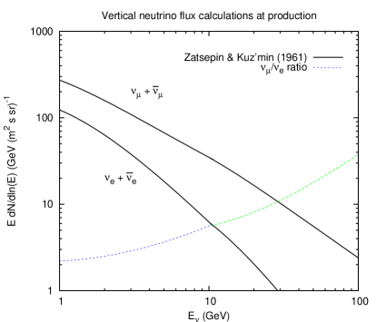
Figure 1: Plots of the numerical formulas of Ref. [2].

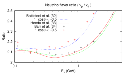
Figure 2: Comparison of the flavor ratio $r$ from three calculations [3, 4, 5].

The first detections of atmospheric neutrinos were made in the early sixties in deep mines by Reines et al. in South Africa [6] and by Menon et al. in the Kolar Gold Fields in India [7]. I have reviewed the history of atmospheric neutrino calculations and measurements in more detail elsewhere [8]. The modern era began in the 1980’s with the construction of large underground detectors to search for proton decay. Interactions of atmospheric neutrinos are most numerous in the GeV range and hence constitute the main background for nucleon decay. Increasingly precise measurements of the atmospheric neutrino beam led to the discovery of oscillations [15] in the $\nu_{\mu}\leftrightarrow\nu_{\tau}$ sector, as is well-known.

After a brief discussion of the current level of uncertainties in the flux of atmospheric neutrinos and the implications for atmospheric neutrinos as a beam for the study of oscillations, I conclude with some comments on atmospheric neutrinos as background for searches for astrophysical neutrinos.

2 Uncertainties in the flux of atmospheric neutrinos

I want to distinguish three approaches to this subject. The first is to compare various calculations of the atmospheric neutrino flux, as in Fig. 2. Other examples of such comparison plots are given in Refs. [8, 9, 10]. There is now a large number of calculations that use different approaches, different interaction models and different representations of the primary cosmic-ray spectrum [3, 4, 5, 11, 12, 13, 14]. The size of differences among the various calculations can be used to guage the uncertainty in the neutrino flux. The general conclusion of such exercises is that ratios agree to better than 5% while the uncertainty in normalization is larger and increases with energy. Differences among the three calculations shown in Fig. 2 for the flavor ratio $r$ are at the level of $2$%.

A related approach [16] is to vary the input parameters within the framework of a single calculational scheme. This approach seeks to avoid the danger of different calculations converging on similar results because they use common input assumptions. Uncertainties in hadronic interaction model dominate at low energy, while uncertainties in the primary spectrum become the dominant source of uncertainty above a few GeV. Within the set of parameters that characterize uncertainties in hadron production, those related to production of pions dominate at lower energy, while uncertainties in strange particle production dominate above 10 GeV, becoming comparable to the uncertainties from the primary spectrum in the TeV region. The importance of kaons is a consequence of the kinematics of meson decay convolved with a steep primary proton beam, which has the effect of making kaon production relatively more important for neutrinos than for muons. For $E_{\nu}>100$ GeV, kaons become the dominant source of atmospheric neutrinos. (See e.g. Fig. 8 of Ref. [9]). For analogous reasons, neutrinos from decay of charmed hadrons must eventually become the most abundant at sufficiently high energy even though charmed hadrons are produced much less often than strange hadrons. At some point (e.g. around several hundred TeV), undertainties in hadro-production of charm will become the biggest source of uncertainty.

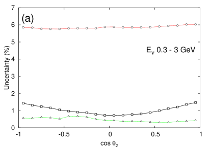
Figure 3: Uncertainties in neutrino ratios as estimated in Ref. [16] ($0.3$-$3$ GeV). (See text.)

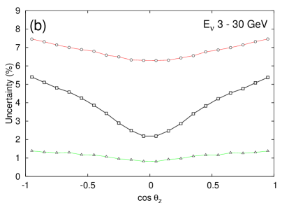
Figure 4: Same as (a) for $3$-$30$ GeV. Lowest curve in (a) and in (b) shows $r$.

Overall uncertainty is at the level of $\pm 15$% in the GeV range, rising to $\pm 40$% for $E_{\nu}=1$ TeV. In contrast, uncertainties in the ratios are much smaller because uncertainties in the primary spectrum and in hadronic interactions cancel in lowest order in the ratios. The uncertainty in the flavor ratio of Eq. 1 is of order $\pm 1$% for $E_{\nu}<30$ GeV, as illustrated in Figs. 4,4. These figures also show the ratios of neutrinos to anti-neutrinos, which are somewhat larger than the uncertainty in $r$ (6-7% for $\nu_{e}/\bar{\nu}_{e}$ and 1-5% for $\nu_{\mu}/\bar{\nu}_{\mu}$) because they are more sensitive to the charge ratio of the parent mesons.

A precise knowledge of the flavor ratio $r$ is particularly important in searching for sub-dominant oscillation effects with atmospheric neutrinos. For example, oscillations driven by the solar parameters are suppressed in the atmospheric neutrino beam by a factor that depends on the near equality of the three neutrino flavors in the oscillated atmospheric neutrino beam [17]. The observed number of $\nu_{e}$ ($N_{e}$) deviates from its value in the absence of solar effects by [17]

$${N_{e}\over N_{e}(0)}\,-\,1\;=\;P_{2}\times(r\,\cos^{2}\theta_{23}\,-\,1),$$ (2)

where $P_{2}(\delta m^{2}_{12}$,$\theta_{12}$) is the two-flavor mixing of $\nu_{e}$ with the orthogonal combination of $\nu_{\mu}$ and $\nu_{\tau}$ [17]. In the sub-GeV region where pathlengths comparable to $R_{\oplus}$ are long enough so that oscillations in the solar parameters can occur, $r$ is close to two. Since the atmospheric mixing is characterized by $\theta_{23}\sim 45^{o}$ and $\cos^{2}\theta_{23}\sim 0.5$, the cancellation is nearly complete. As shown in Fig. 2, however, $r_{\rm sub-GeV}$ is somewhat larger than two (more so for atmospheric neutrinos in the vertically upward quadrant of phase space, which have pathlength $>R_{\oplus}$), making a measurement of the octant of $\theta_{23}$ possible in principle with sufficient statistics.

A similar suppression factor occurs in the atmospheric neutrino beam for effects that depend on the deviation of $\sin^{2}\theta_{13}$ from zero [18]. Such effects are, however, expected to be most important for $E_{\nu}\sim 5$ GeV [18], where the flavor ratio is already significantly larger than two. In this case, the limiting factor is the intrinsically small size of $\sin^{2}\theta_{13}$ [18].

A different and complementary approach to determining the flux of atmospheric neutrinos accurately is to consider the analysis of the data of Super-K I [19] as a measurement of the flux of atmospheric neutrinos. The Super-K analysis proceeds by simultaneously fitting their data with the oscillation parameters together with a large set of parameters that characterize experimental and theoretical uncertainties. The theoretical parameters reflect deviations from the assumed production spectrum of atmospheric neutrinos (i.e. before oscillations). Shifts in the fitted parameters that describe the trial production spectrum of atmospheric neutrinos can be considered as a measurement of the atmospheric neutrino flux at production. This approach may be of greatest value for $E_{\nu}\sim 100$ GeV to $1$ TeV, because the normalization and oscillation parameters are primarily determined by the data at lower energy. In this regard, the adjustment of the spectral index found in the Super-K fit suggests that the neutrino spectrum continues into the high-energy range at a higher level than some calculations. A recent analysis [20] confirms this conclusion, as does the new analysis of Honda et al. [21].

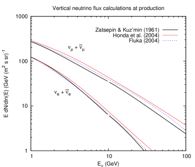
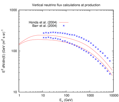
Figure 5: Neutrino flux from several calculations. The right panel shows muon neutrinos only, with $\nu_{\mu}$ and $\bar{\nu}_{\mu}$ plotted separately for each calculation. (Note the difference in energy ranges and powers of $E$ in the two plots.)

3 Background for astrophysical neutrinos

Neutrino telescopes designed to search for astrophysical neutrinos generallly have thresholds in the range of $\sim 100$ GeV or higher. Figure 5 is a compilation of several calculations, incuding two that extend to high energy. The hard spectral index that comes out of the Super-K analysis [19] suggests that higher intensities should be preferred in the TeV region. The much larger ratio of $\nu_{\mu}\,/\bar{\nu}_{\mu}$ in Ref. [5] as compared to that of Ref. [4] reflects the large associated production ($p\rightarrow\Lambda\,K^{+}$) assumed by Barr et al. [5] at high energy. The production of strange and charmed particles is a significant source of uncertainty and needs more investigation. Decay of charmed hadrons is expected to become the dominant source of atmospheric neutrinos at sufficiently high energies, $\sim 100$ TeV. At some level it will become the limiting factor in a search for a diffuse flux of extra-terrestrial neutrinos.

A well-understood feature of the atmospheric neutrino flux that may be useful in distinguishing signal from background is its characteristic dependence on zenith angle. A standard form for the differential spectrum of $\nu_{\mu}\,+\,\bar{\nu}_{\mu}$ at high energy is

$$\phi_{\nu}(E_{\nu})\;=\;{\phi_{N}(E_{\nu})\over 1\,-\,Z_{NN}}\times\Sigma_{i=1}^{3}\,{A_{i}\over 1+B_{i}\cos\theta E_{\nu}/\epsilon_{i}},$$ (3)

where the three terms correspond respectively to neutrinos from decay of pions, kaons and charmed hadrons. The overall flux is proportional to the primary spectrum of nucleons, $\phi_{N}(E_{\nu})$, evaluated at the energy of the neutrino and scaled by a factor $1/(1-Z_{NN})$ related to the nucleon attenuation length. Each flavor of hadron has a characteristic critical energy, $\epsilon_{i}$, above which the hadron is more likely to interact than to decay. The shape of each contribution also depends on a numerical factor ($B_{i}$) and on the cosine of the zenith angle. The latter is the “secant theta” effect. For $E_{\nu}>>\epsilon_{i}/(B_{i}\cos\theta)$ the contribution is inversely proportional to $\cos\theta$ and asymptotically one power of energy steeper than the primary spectrum. At very large angles ($\sim\theta>70^{o}$) the secant theta term is limited by the curvature of the Earth.

Neutrinos from astrophysical sources do not depend on the local zenith angle at which they are observed. Therefore in principle the known zenith angle dependence of the atmospheric background is available as an extra parameter to distinguish background from signal. The most obvious example would be the contrast between atmospheric background and an isotropic, diffuse extraterrestrial flux of high-energy neutrinos. Because the contribution from charm is also isotropic (until extremely high energy), the distinction disappears when the intensity of the extraterrestrial neutrinos is at the level of atmospheric neutrinos from decay of charmed hadrons.

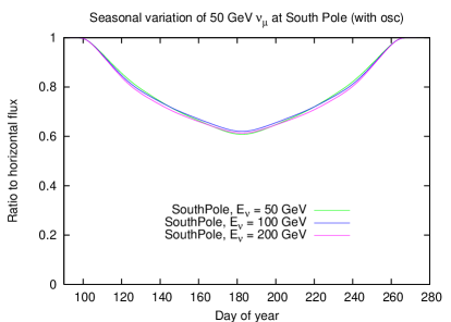
Figure 6: Relative variation of the intensity of atmospheric $\nu_{\mu}+\bar{\nu}_{\mu}$ from the direction of the Sun as viewed from the South Pole during Austral winter (including oscillations).

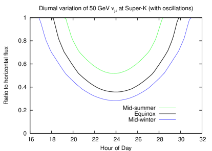
Figure 7: Relative variation of the intensity of $50$ GeV atmospheric $\nu_{\mu}+\bar{\nu}_{\mu}$ from the direction of the Sun as viewed from Super-K, including oscillation effects.

For point sources of neutrinos observed from mid-latitude detectors, variation of the background in the direction of a potential source as it rises and sets can in principle also help to distinguish background from signal. A related example is the indirect search for neutrinos from WIMP annihilation in the Sun. Figures 77 show the expected diurnal variation of the atmsopheric background from the direction of the Sun as seen from the South Pole and from Super-K.

References

- [1] Zatsepin, G.T. & Kuz’min, V.A. Sov. Phys. JETP 12, 1171 (1961).
- [2] Zatsepin, G.T. & Kuz’min, V.A. Sov. Phys. JETP 14, 1294 (1962).
-
[3]
Battistoni, G. et al., Astropart. Phys. 19, 269 (2003) (Erratum pp 291-294).
http://www.mi.infn.it/battist/neutrino.html -
[4]
Honda, M. et al., Phys. Rev. D 70, 043008 (2004).
http://www.icrr.u-tokyo.ac.jp/mhonda/ -
[5]
Barr, G.D. et al., Phys. Rev. D 70, 023006 (2004).
http://www-pnp.physics.ox.ac.uk/barr/fluxfiles/ - [6] Reines, F. et al., Phys. Rev. Letters 15, 429 (1965).
- [7] Achar, C.V. et al., Phys. Lett. 18, 196 (1965).
- [8] T.K. Gaisser, Physica Scripta T121 (2005) 51 (astro-ph/0502380).
- [9] T.K. Gaisser, Nucl. Phys. B (Proc. Suppl.) 118 (2003) 109.
- [10] Giles Barr, Nucl. Phys. (Proc. Suppl.) 143 (2005) 89.
- [11] Wentz, J. et al., Phys. Rev. D 67, 073020 (2003).
- [12] Liu, Y. et al., Phys. Rev. D 67, 073022 (2003).
- [13] Favier, J. et al., Phys. Rev. D 68, 093006 (2003).
- [14] See T.K. Gaisser & M. Honda, Ann. Revs. Nucl. Part. Sci. 52 (2002) 153 for a review of earlier calculations.
- [15] Fukuda, Y. et al., Phys. Rev. Lett. 81, 1562 (1998).
- [16] G. Barr et al., Phys. Rev. D74 (2006) 094009.
- [17] O.L.G. Perez & A. Yu. Smirnov, Nucl. Phys. B456 (1999) 204 and B680 (2004) 479.
- [18] S.T. Petcov & T. Schwetz, Nucl. Phys. B740 (2006) 1.
- [19] Ashie, Y. et al., Phys. Rev. D 71 (2005) 112005.
- [20] M.C. Gonzalez-Garcia, M. Maltoni & J. Rojo, hep-ph/0607324.
- [21] M. Honda et al., astro-ph/0611418.