Microvariability of Line Profiles in the Spectra of OB Stars II: $\delta\,$Ori A

A.F.Kholtygin^1,∗, T.E.Burlakova^2,3, S.N.Fabrika³, G.G.Valyavin^2,3, M.V.Yushkin³

Abstract–We have studied variability of the spectral lines of the OB star $\delta\,$Ori A–the brightest component of the $\delta\,$Ori triple system. Forty spectra with signal-to-noise ratios $\approx$500–800 and a time resolution of four minutes were obtained. We detected variability in the HeII$\,\lambda\,4686$, HeI$\,\lambda\,$4713 and H$\beta$ absorption and the CIII$\,\lambda\,$5696 emission line profiles. The amplitude of the variability is $\approx$(0.5–1)% of the continuum intensity. The dynamical wavelet spectrum of the profile variations reveals large-scale components in the interval 25–50 km/s that move within the -$V\sin i$ to $V\sin i$ band for the primary star of the system, Aa¹, with a band crossing time of 4^h–5^h. However, some of the variable features go outside the band, presumably due to either imhomogeneities in the stellar wind from $\delta\,$Ori Aa¹ or non-radial pulsations of the weaker components of the system, Aa² or Ab. The detected variability may by cyclic with a period of $\approx 4^{h}$ . We suggest that it is associated with non-radial pulsations of the primary in the sector mode $(l,m)=(2,-2)$.

1 Introduction

Spectral observations of hot stars at UV [1, 2], optical [1, 3, 2, 5, 4, 6], and X-ray [7, 8] wavelengths indicate the presence of structures in the atmospheres of these stars with various sizes and densities, and with lifetimes from less than an hour to several days. Variations of the line profiles in the spectra of OB stars are mainly regular or quasi-regular. The spectra of B stars and six O stars display regular short-period (3 – 12 h) profile variations for numerous lines (in particular, HeI) associated with the non-radial pulsations of these stars [6].

Weak magnetic fields (several hundred Gauss at the stellar surface) may be one factor favoring the formation of large-scale structures in the atmospheres of O stars[9]. Currently, magnetic fields have been detected with sufficient reliability only in one O star, $\theta^{1}\,$Ori C [10], and several early B subtype stars[11]. Unlike Bstars, the amplitudes of the line profile variations in the spectra of O stars are relatively small (1%–3%; see, for example, [12]), so it it is more appropriate to call this line profile microvariability. To detect such variability and to clarify its nature, observations with high time and spectral resolution and high signal-to-noise ratios ($\geq 300$) are needed.

Here, we continue our study of the microvariability of hot stars begun in [12], when we analyzed line- profile variability in the spectra of the supergiants 19 Cep, $\alpha\,$Cam $\lambda\,$Ori A (O9.5II).

We now present the results of spectral observations of the spectral triple system $\delta\,$Ori A, whose primary displays the same spectral type as $\lambda\,$Ori A – O9.5. Section 2 contains general information about the $\delta\,$Ori A system, and Section 3 describes the observations and reduction of the spectra. Section 4 presents the methods used in and the results of our analysis of line-profile variability in the spectrum of $\delta\,$Ori A.. Our interpretation of the observations is presented in Section 5, followed by a brief conclusion section.

2 THE $\delta\,$Ori A SYSTEM

$\delta\,$Ori is a wide visual triple system containing three components: A (HD 36486), B (Bd–00^∘.983B), and C (HD 36485), with apparent visual magnitudes of 2.23^m, 14.0^m, and 6.85^m, respectively. Components Band C are at distances of 33”. and 53”, respectively, from the primary component, A. Our observations refer to the brightest component $\delta\,$Ori A.

Table 1: Parameters of the $\delta\,$Ori A system

	Components
Parameter	Aa1	Aa2	Ab	References
Distance to the star, pc	360	360	360	[15]
Distance to component Aa1, $R_{\odot}$	…	33	$\approx{25\,000}$	[8]
Spectral type	09.5II	B0.5III	B (early subtype)	[14]
Orbital period	—	$5.7325\,$ days	$\approx 200\,$ yrs	[14]
Radius, ($R_{\odot}$)	11	4	…	[14, 8]
Mass, ($M_{\odot}$)	11.2	5.6	$\approx 27$	[14]
Luminosity, $\log(L/L_{\odot})$	5.26	4.08	-
$T_{eff}$, K	33 000	27 000	…	[16, 17]
$\lg g$	3.4	3.8	…	[16, 17]
Contribution to optical radiation	70	7	23	[14]
in HeI$\,\lambda\,6678\,$ line region, (%)
$V\sin i$ (km/s)	$157\pm 6$	$138\pm 16$	$\approx 300$	[14]
	$133$			[18]
$V_{\infty}$, km/s	2000	1500	…	[19, 20]
Mass loss ${\dot{M}},~{}M_{\odot}/\mbox{yr}$	$1.1\times 10^{-6}$	$1.2\times 10^{-7}$	…	[19, 20]

$\delta\,$Ori A (HD 36486, HR 1852) is a physical triple system with the primary $\delta\,$Ori Aa, which is an eclipsing binary with orbital period P =5.73^d  [13], and the secondary $\delta\,$Ori Ab, with an orbital period of 224.5 yrs. Recent detailed Doppler tomography studies [14] have made it possible to refine the parameters of the .Ori A triple system, presented in the Table.

The brightest component, $\delta\,$Ori Aa¹, is a high-mass O9.5II star with an intense stellar wind; the star’s mass-loss rate is $\log(\dot{M})\approx-6.0$ and the limiting velocity of the wind is $V_{\infty}\approx 2000\,$km/s. A value a factor of two lower is given in [21]: $\lg(\dot{M})\approx-6.3$. According to [22, 16], $V_{\infty}\approx 2300\,$ / . The rotational velocities of the star determined by different authors differ appreciably. In  [14], a relatively high rotational velocity for the primary was obtained, $V\sin i=157\pm 6\,$km/s,, while Abt et al. [18] found $V\sin i=133\,$km/s (see the Table).

The study [16] presents a photospheric radius for the primary, Aa¹ $R_{*}=22R_{\cdot}$,, twice the value $R_{*}=11R_{\cdot}$, given in the Table. This discrepancy is probably due to the fact that a larger distance to the star was used in [16] than the distance in the Table, 450 pc.

The component $\delta\,$Ori Aa² is a B0.5 III star. Preliminary studies indicate that the third component of the system, $\delta\,$Ori Ab, is an early B-subtype star with broad spectral lines, indicating either a high rotational velocity ($V\sin i\approx 300\,$km/s) or binarity of the star [14].

Harvin et al.  [14] determined the orbital inclination of the $\delta\,$Ori Aa close binary to be $i\approx 67^{o}$ and estimated the mass of the components to be M(Aa${}^{1})=11.2M_{\odot}$ and M(Aa${}^{2})=5.6M_{\odot}$. The secondary, $\delta\,$Ori Aa², is appreciably weaker than the primary (see Table). Both the primary and secondary, Aa¹ and Aa², have masses roughly half the mass of main-sequence stars with corresponding positions on the HR diagram [14].. It was suggested in [14]. that, in the course of its evolution, the system underwent a common- envelope stage in which both stars filled their Roche lobe and with intense mass loss. After the system had lost half its total mass, the distance between the components increased and the mass loss ceased.

The mass of the third component of the system, Ab, cannot be derived from the radial velocities. The Table presents the value $M(Ab)\approx 27\,M_{\odot}$ from [14], which corresponds to a main-sequence star with $M_{\mbox{\scriptsize bol}}=-4^{m}.2$. A main-sequence star with a mass of $27\,M_{\odot}$ should have spectral type O8.5V[23], which contradicts the spectral classification in the Table. To explain this inconsistency, Harvin et al. [14] suggest that Ab may be a close binary consisting of two main- sequence B0.5V stars with a mass of $\approx 19\,M_{\odot}$.

3 OBSERVATIONS AND REDUCTION OF THE SPECTRA

Our spectral observations of the $\delta\,$Ori A system were carried out on January 10/11, 2004 with the 6m telescope of the Special Astrophysical Observatory as part of our program to search for rapid line-profile variability in the spectra of early-type stars [12]. We used the NES quartz echelle spectrograph [24], which is permanently mounted at the Nasmyth focus and equipped with the Uppsala 2048 x 2048 CCD. To increase the spectrograph’s limiting magnitude, we used a three-cut image cutter [25]. The resulting spectral resolution was $R~{}\approx~{}60000$ and the dispersion 0.033 A/pixel. The image size during the observations was about 3”. The reference spectrum was provided by a ThAr lamp.

The angular separation between the most distant components, $\delta\,$Ori Aa¹ and Ab, is about 0.3”. (see Table), which means that all components contribute to the resulting spectrum of the $\delta\,$Ori A system. Over a total observation time of $\approx 2^{h}50^{m}$, we obtained 40 spectra of the star with an exposure time of 180 s. Taking into account the CCD readout, the time resolution was 260 s. The signal-to-noise ratio per pixel . was 500 in the blue (4500 Å) and 800 in the red . (6000 Å).

The preliminary reduction of the CCD echelle spectra was done in the MIDAS package [12]. We adapted the standard ECHELLE procedures of the MIDAS package for data obtained with an image cutter. The reduction stages included
1) median filtering and averaging of the bias frames with their subsequent subtraction from the remaining frames; 2) cleaning of cosmic rays from the frames; 3) preparation of the flat-field frame; 4) determination of the position of the spectral orders (using the method of Ballester [26]); 5) subtraction of scattered light (to determine the contribution of scattered light, we distinguished the inter-order space in the frames, and then carried out a two-dimensional interpolation; this function was recorded in individual frames to be subtracted from the initial images); 6) extraction of the spectral orders from the reduced images of the stellar spectrum, the flat fields, and the wavelength reference spectra; flat-field reduction; 7) wavelength calibration using a two- dimensional polynomial approximation for the identifications of the lines of the reference spectrum in various spectral orders.

When the image cutter is used, each order of the echelle image is represented by three sub-orders (cuts). In a given order, the instrumental shift of the upper and lower cuts relative to the middle cut was determined via a cross-correlation with the reference spectra. The three cuts obtained in a given order were summed using median averaging, taking into account the determined instrumental shifts.

To study the line profile variability, the processed spectra were normalized to the continuum level reconstructed in each echelle order. We drew the continuum in spectral orders containing narrow spectral lines using the technique developed by Shergin et al. [27], in which spectra are smoothed with a variable Gaussian filter with a 25-30 Åwindow, with the same parameters for the entire set of spectra.

In orders containing broad (usually hydrogen) spectral lines, the continuum was drawn using the following procedure. In all 40 spectra, broad lines were cut out in fixed wavelength intervals. To determine the position of the continuum, we used a polynomial approximation for all wavelengths of the order, except for the regions of the cut-out broad spectral lines. The approximation parameters remained unchanged for all spectra of the set. This procedure provides stability and reproducibility of our determination of the continuum in all the spectra with an accuracy of up to several tenths of a percent. This makes it possible to reach high accuracy in deriving the differential line profiles and detecting profile variability in broad lines at levels down to 0.1%.

4 LINE PROFILE VARIABILITY

4.1 Contribution from Different Components of the System to the Line Profiles

We selected sufficiently strong unblended lines for detailed studies of the line-profile variations. The selection criterion for absorption lines was that the residual intensity be $r_{\mbox{\scriptsize max}}>0.1$. These criteria led to the selection of the HeII$\,\lambda\,$4686, HeI$\,\lambda\,$4713 and H_β lines. In addition, we studied the profiles of the CIII$\,\lambda\,$5696 emission line.

The $\delta\,$Ori A system contains three O and B stars, each of which could have variable line profiles; the observed profiles result from the contributions of all stars. It follows from the Table that above two-thirds of the flux from the system at the wavelength of the HeI$\,\lambda\,6678\,$ line comes from the primary component, Aa¹. The contributions from Aa² and Ab at these wavelengths are substantially smaller.

At other wavelengths, the contributions from Aa² and Ab may differ from those in the Table. To determine to what extent each of the stars in the system is responsible for line-profile variability, the contribution of each star to the total profiles of the analyzed lines must be clarified. In addition, taking into account the substantial scatter of the $V\sin i$ values for Aa¹ (see the Table), reliable v sin i estimates for the components of the $\delta\,$Ori A system are highly desirable.

Figure 1: HeII.4686 synthetic (bold curve) and observed (thin curve) line profiles, plotted in terms of the Doppler shift V from the line center.

To solve these problems, we modeled the combined profiles for the photospheric HeII$\,\lambda\,$4686 and HeI$\,\lambda\,$4713 lines in the spectrum of $\delta\,$Ori A. We assumed the total line profile to be the sum of the contributions from the components, since Aa¹ and Aa² are not eclipsed at the above orbital phases. We calculated the rotation-broadened line profiles using the standard relations (see, for example,[28]). The radial velocities of the components for the time of the observations were calculated using the ephemeridas of Harvin et al. [14].

During our observations, the orbital phase varied in the narrow interval $0.848-0.851$. For such small phase variations, the velocities of the components can be considered to be constant over the total observation time. The heliocentric velocities $V(\mbox{Aa${}^{1}$})=-21\,$km/s, and $V(\mbox{Aa${}^{2}$})=-102\,$km/s were obtained using the ephemeris [14].

For convenience in comparison, both the calculated and observed line profiles were transformed into the system of the center of mass of the close binary $\delta\,$Ori Aa. The velocity $V_{\mbox{\scriptsize r}}=\approx 23.0\,$ /  [14] was used as the zero-point of the velocity scale. In this system, the velocity of the third component is $V(\mbox{Ab})=\approx 27\,$km/s [14].

Figure 1 presents the total profile of the photospheric HeII$\,\lambda\,4686$ line calculated using these parameters. The observed profiles are reproduced very reasonably. The small discrepancies between the observed and calculated profiles near $V=150-250\,$km/s may be due to the contribution of the stellar wind from Aa¹.

4.2 Variations of the Average Profiles. Differential Profiles

The nightly-average line profiles in O-star spectra are often substantially variable [6]. Line-profile variations on shorter time intervals are insignificant. To make the line-profile variations in the spectra of $\delta\,$Ori A in time intervals of 30-40 min more clearly visible, we divided the profiles into four groups with ten profiles in each and calculated the average profiles for these groups.

The average profiles for each group presented in Fig. 2 display appreciable variations within an hour. These variations are particularly clearly visible in the HeI$\,\lambda\,$4713. In the transition from the first group of spectra to the following three groups, the line depth decreases by 1%-1.5%. These variations are correlated with variations in the groups of average profiles for the CIII$\,\lambda\,$5696 emission line. In the transition from the first to the fourth group of profiles, the flux in the central region of the line increases by $\approx 1\%$.The amplitude of the flux variations in the H_β and HeII$\,\lambda\,$4686 lines reaches 1%-2%.

In the blue wing of the CIII$\,\lambda\,$5696 profile, narrow absorption features with depths less than 0.01 of the continuum intensity can be seen. Similar, but less deep, features are also present in the red wing of the line. Our analysis shows that the positions of all of these features coincide with those for atmospheric absorption lines, primarily water vapor [29].

Figure 2: Average profiles for spectra 1-10 (thin solid curve), 11-20 (dashed curve), 21-30 (bold solid curve), and 31-40 (dotted curve) for the HeII$\,\lambda\,$4686 (top left), HeI$\,\lambda\,$4713 (top right), H_β (bottom left), and CIII$\,\lambda\,$5696 (bottom right) lines. The flux in the line frequencies, $F$, is given as a fraction of the flux in the continuum adjacent to the lines, $F_{\rm c}$. The arrows indicate the laboratory wavelengths of the lines.

To reveal variable features in the line profiles, we constructed differential profiles by subtracting the average profile obtained using all forty available spectra of $\delta\,$Ori A from the individual profiles.

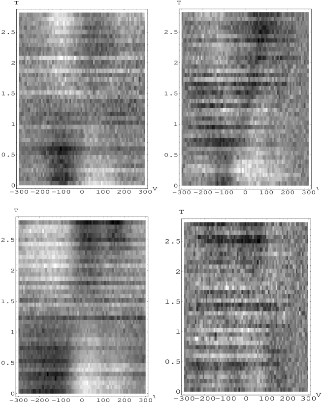
Figure 3 presents dynamical differential profiles of the studied lines in the spectrum of $\delta\,$Ori. Grey shades indicate deviations of individual profiles from those averaged over the entire set of spectra. For convenience, the wavelength scale is translated into Doppler shifts from the line center. The radial velocity of the center of mass of the $\delta\,$Ori A system was used as the zero point of the wavelength scale (see Section 4.1).

We show the differential profiles in the ”negative”, i.e., darker regions in Fig.3correspond to regions of the profile that lie above the average value (peaks), while lighter regions correspond to parts of the profile that lie below the average value (valleys). This makes it easier to identify regular variations of the profiles in Fig.3. The HeII$\,\lambda\,$4686, HeI$\,\lambda\,$4713, and H_β line profiles show that the peaks move from the violet to the red wing of the profile.

We can see a broad (50-100 km/s), variable feature in the vicinity of the HeII$\,\lambda\,$4686 line. The feature appears at a velocity near -100 km/s in the first (lower) differential profiles, and is then gradually shifted towards the line center. In the last (upper) profiles, it is visible in the domain of positive velocities. Such behavior of features in the differential profiles is typical for non-radial pulsations [30]. Virtually no obvious spectrum-to-spectrum profile variations near weaker spectral lines, due to both the short duration of the observations and the low amplitude of the profile variations. We used the technique described in the following subsection to reveal profile variations in such weak lines.

Figure 3: Dynamical spectra for the profile variations for the HeII$\,\lambda\,$4686 (top left), HeI$\,\lambda\,$4713 (top right), H_β (bottom left), and CIII$\,\lambda\,$5696 (bottom right) lines. The interval between consecutive spectra is four minutes. Dark regions in the diagrams correspond to intervals brighter then the average profile (peaks), and light regions to less bright intervals (valleys).

4.3 Analysis of the Spectrum of Time Variations of the Differential Spectra

The method of Fullerton et al. [31] is often used to elucidate the presence of weak line profile variability. We describe here a substantially modified version of this technique, which we used in our analysis. Suppose that N spectra of a studied star have been obtained. We denote $F_{i}(\lambda),~{}i=1,...N$ to be the flux in the ith spectrum at wavelength ., normalized to the continuum. Let $\overline{F}_{i}(\lambda)$ be the flux at wavelength $\lambda$ averaged over all the observations. The dispersion of the random ${F}_{i}(\lambda)$ is then equal to

$$D(\lambda)=TVS(\lambda)$$

$$=\frac{1}{N-1}\left(\sum\limits_{i=1}^{n}g_{i}\left[F_{i}(\lambda)-\overline{F}_{i}(\lambda)\right]^{2}\left/{\sum\limits_{i=1}^{n}g_{i}}\right.\right)\,$$ .

Here, $g_{i}$ is the relative weight of the $i$th observation, which is inversely proportional to $\sigma_{i}^{c}$ – the standard deviation $\overline{F}_{i}(\lambda)$ at wavelengths near the line whose profile variability is being studied. This definition for $g_{i}$ makes it possible to take into account the different qualities of the data in the analyzed set of spectra. $TVS(\lambda)$, or the Time Variation Spectrum [31], obeys a $\chi^{2}/(N-1)$ distribution with $N-1$ degrees of freedom.

In the case of profile variability with a sufficiently high amplitude, the $TVS(\lambda)$ in the vicinity of the corresponding line substantially exceeds its values in the adjacent continuum. To ensure that the increase in the amplitude is due to real variability, we specified a small significance level $\alpha\ll 1$ for the hypothesis that the excess is due to a random variation of the noise component of the profile. The quantites for the $\chi^{2}$ distribution are calculated in the ordinary way for this $\alpha\ll 1$ level (see, for example, [32]). Let $\chi^{2}_{\alpha}$ be specified so that the probability $P(\chi^{2}/(N-1)>\chi^{2}_{\alpha})=\alpha$ If the calculated $TVS(\lambda)$ value exceeds $\chi^{2}_{\alpha}$, the hypothesis that the line profile is variable can be adopted.

As was noted in [12], for lines with small-amplitude profile variations or with a small number of spectra, the function $TVS(\lambda)$ cannot be used to prove whether a given line profile is variable. In the absence of any visible variations, we determined whether a line profile was indeed variable using the following procedure.

Before the standard-deviation spectrum was obtained, the differential spectra were pre-smoothed using a filter that is broad compared to the pixel size. If the filter width is $\Delta\lambda$ on the wavelength scale, then the amplitude of the smoothed random (noise) component of the differential profiles $\overline{N_{j}(t)}$ decreases after smoothing by a factor of $\approx\sqrt{\Delta\lambda/\delta\lambda}$, where $\delta\lambda$ is the width of an individual pixel on the wavelength scale in the vicinity of the line. If the width of the variable component is not smaller than that of the filter, then smoothing with this filter will not substantially change the amplitude of the variable component, while, after the smoothing, peaks in the standard deviation spectrum that correspond to the variable component can be detected with increased reliability.

It was shown empirically that the best results are obtained for smoothing with a Gaussian filter with a width of $S=0.5-1.0$ Å (15-30 pix.). To more clearly demonstrate the method used to search for weak profile variations, we used a smoothed time-variation spectrum, smTVS, which is a collection of spectra of the normalized standard deviation $\sigma(\lambda,S)=\sqrt{TVS(\lambda,S)}$ with the differential spectra smoothed with a Gaussian filter with a variable width $S$.

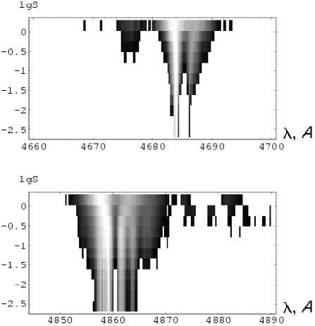
Figure 4 presents density diagrams for the time-variation spectra for the HeII$\,\lambda\,$4686 and H_β line profiles. Darker areas correspond to higher amplitudes of the smTVS spectrum. Only values corresponding to significance levels $\alpha<10^{-4}$ for the hypothesis that the profiles are not variable are presented. The density diagrams show that the variability of the H_β and HeII$\,\lambda\,$4686 lines is clearly present.

The smTVS spectrum for the HeII$\,\lambda\,$4686 line profile with the filter width $S>0.3\,$Åindicates variability of the CIII$\,\lambda\,$4673.95, OII$\,\lambda\,$4673.75, 4676.234, NII$\,\lambda\,$4674.909, 4678.14, and SiIII$\,\lambda\,$4673.273 lines, which cannot be detected using ordinary methods. With larger filter widths, variability of a large group of OII, NIII, and ArII lines at wavelengths from. 4871 to 4890 Åbecomes visible. Note that, in spite of the fact that these lines are extremely weak and their residual intensities do not exceed the noise level (by one pixel along the spectrum) at the adjacent continuum, their variability is clearly detected. Unfortunately, our technique cannot be used to localize weak lines with variable profiles accurately when larger filter widths are used.

Figure 4: Time variation spectrum for the HeII$\,\lambda\,$4686 (top) and H_β (bottom) line profiles. The vertical axis plots the logarithm of the filter width in Å.

Note that the efficiency of this method of using the smTVS spectra to search for weak line-profile variability is sensitive to the number of spectra obtained, and increases substantially as this number increases.

4.4 Wavelet Analysis for the Line-Profile Variations

Analysis of the differential line profiles in the spectra of a star (Fig. 3) indicates the presence of a number of discrete features. Many small-scale features are connected with the noise component of the profiles, whereas larger-scale features may be due to the regular component of the profile variations[12]. A very suitable mathematical technique for studying the development of different-scale profile features is wavelet analysis (see, for example,[33, 5]). It is advisable to use as the analyzing (or mother) wavelet the so- called MHAT wavelet, $\psi(x)\!\!=\!\!(\!1-x^{2})\!\exp(\!-x^{2}/2)\,,$ which displays a narrow energy spectrum and whose zero and first momenta are equal to zero. The MHAT wavelet is essentially the second derivative of a Gaussian function (taken with a minus sign) that can be used to describe features in the differential line profiles.

Using this wavelet, the integral wavelet transformation can be written[33, 34]:

$$W(s,u)=\frac{1}{s}\int\limits_{-\infty}^{\infty}f(x)\psi\left(\frac{x-u}{s}\right)dx$$

$$=\,\int\limits_{-\infty}^{\infty}f(x)\,\psi_{su}(x)dx \,.\qquad$$

where $f(x)$ is the studied function (in our case, a differential line profile). The signal energy energy, $E_{W}(s,u)\!\!=\!\!W^{2}(s,u)\!$, characterizes the energy distribution of the studied signal in $(s,u)=\,$= (scale, coordinate) space. Further, we will analyze the differential line profiles in the form $r(V)=F_{i}(V)-\overline{F}_{i}(V)$,where the Doppler shift $V$ from the central frequency of the line is used as the x coordinate. In this case, the scale variable $s$ is expressed in km/s.

To study the evolution of features in the differential profiles, we calculated wavelet spectra, $W(s,V)=W(s,V,t)$, for the HeII$\,\lambda\,$4686, HeI$\,\lambda\,$4713, H_β and the CIII$\,\lambda\,$5696 emission line for all times $t$ corresponding to our spectra. We will call the collection of functions $W(s,V,t)$ the dynamical wavelet spectrum for the differential line profiles.

Figure 5 presents density diagrams for the dynamical wavelet spectra of the studied lines for the scale parameter $s=50\,$km/s. The diagrams present the ratios $d=(W-W_{min})/\Delta W$ rather than the function $W(s,V,t)$ itself. Here, $\Delta W=W_{max}-W_{min}$, where where $W_{max}$ and $W_{min}$ are the maximum and minimum of $W(s,V,t)$ for all possible $t$ in the interval of $V$ within the line profile. Darker regions correspond to larger values of $W(s,V,t)$. We have marked only the values for the parameter $d\geq d_{cut}$ – the cutting parameter of the wavelet spectrum. In Fig. 5 dcut =0.6.

Figure 5: Dynamical wavelet spectrum of the HeII$\,\lambda\,$4686 (top left), HeI$\,\lambda\,$4713 (top right), H_beta (bottom left), and CIII$\,\lambda\,$5696 (bottom right) line-profile variations for the scale parameter $S_{0}$=50 km/s. The corresponding line profiles averaged over the entire set of observations are given beneath the wavelet spectra. The dotted curve indicates the region $\pm V\sin i$ for the primary component Aa¹ of the $\delta\,$Ori A system.

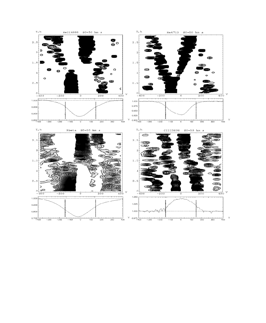
For a comparison, the average line profiles are placed beneath the wavelet spectra diagrams. In the average profiles, the dotted lines delineate the region $-V\sin i\div V\sin i$ for the primary, Aa¹ (see Table).

We can see in Fig. 5 that all the wavelet spectra display broad structures moving along the line profiles, with features moving from the violet to red edge of the line being most prominent. The same type of features are visible in the wavelet spectra of the absorption HeII$\,\lambda\,$4686, HeI$\,\lambda\,$4713 and H_β differential line profiles, moving from $-110\div-100\,$km/s to $\approx 100\div 110\,$km/s over the total observation time, $2^{h}\,50^{m}$. The estimated crossing time $T_{\mbox{\scriptsize{cross}}}$ for the entire band of $-V\sin i\div V\sin i$ is $\approx 4^{h}$. Note the similarity between the dynamical wavelet spectrum and the time variation spectrum for the line profiles (see Section 4.2).

The HeI$\,\lambda\,4713$ and HeII$\,\lambda\,4686$ lines are basically formed in the photosphere, and their dynamical wavelet spectra behave in a very similar way. Apart from the primary, which shifts towards the red part of the line profile, another, weaker, component is seen. This secondary component appears $\approx 40$ min after the start of the observations at $\approx-130\div\-150\,$km/s and moves towards more negative velocities ($\approx-300\,$300km/s) by the end of the observations. This feature may correspond to component Ab of the $\delta\,$Ori A system, since profile variations associated with possible pulsations of this star should be traced up to $V=V_{min}\approx-300\,$km/s (see the Table). It is also possible that this feature is formed in the powerful stellar wind from the primary of the $\delta\,$Ori A system.

The same secondary component as that seen for the HeI$\,\lambda\,4713$ and HeII$\,\lambda\,4686$ lines (although less distinctly pronounced) is also present in the dynamical wavelet spectrum of the H_β line. Appreciable features of the dynamical wavelet spectrum of H_β are visible even beyond the $\pm V\sin i\approx 300\,$km/s band for the most rapidly rotating star, Ab, probably indicating that the intense stellar wind from the primary contributes substantially to the H_β line profile.

The dynamical wavelet spectrum of the differential we can see two main features, moving almost parallel profiles of the CIII$\,\lambda\,5696$ emission line differs appreciably from those for the absorption lines. In Fig. 5 we cam see two main features, moving almost parallel in the $-200\div 200\,$km/s band from the red to the violet part of the line profile.

Figure 6: Dynamical wavelet spectrum of the HeI$\,\lambda\,$4713 line profile variations for $s_{0}$ =25 km/s and various cutting parameters $d_{c}ut$ = (a) 0, (b) 0.5, (c) 0.6, (d) 0.65, (e) 0.7, (f) 0.75.

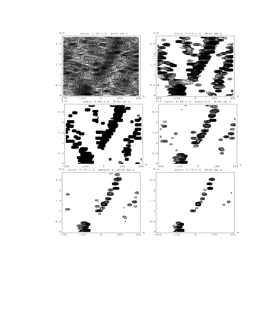
Regular structures in the wavelet spectra are most clearly visible in the profile of the HeI.4713 line. To study these structures in detail, Fig. 6 presents the calculated dynamical wavelet spectrum for this line for the wavelet-spectrum cutting parameters $d_{cut}$ = 0, 0.5, 0.6, 0.65, 0.7, 0,75 and for $S_{0}=25\,$km/s. As $d_{cut}$ increases, more pronounced structures of the wavelet spectrum become more dominant. All the wavelet spectra display movement of a feature from -120 to 90 km/s; for $d_{cut}\geq 0.75$, only this main feature is present in the wavelet spectrum.

To clarify the nature of the features revealed in the wavelet spectra for the differential profiles, we must determine whether the line profile variations related to these features are regular. We consider this question in the following section.

4.5 Search for Regular Variability

To search for periodic profile variations, we carried out a Fourier analysis of the line-profile variability in the spectrum of $\delta\,$Ori A. The Fourier spectra were cleaned of false peaks using the CLEAN [35] procedure modified by Vityazev [36].

For each of the studied lines, we constructed the time series $\Delta F(t,\lambda)$ of differential fluxes for a given profile at time $t$ for a given $\lambda$. For convenience, the $\lambda$ values were converted into Doppler shifts $V$ from the profile center in the center-of-mass frame of the $\delta\,$Ori A triple system (see Section 4.1).

This CLEAN procedure was applied to all the observed $V$ values along a line profile. To smooth the noise component of the profile variations, the $\Delta F$ values were averaged within a spectral window with width $\Delta V$ = 5-6 km/s. Our calculations showed that our specific selection of $\Delta V$ do not appreciably influence the resulting Fourier spectra.

Figure 7: Fourier power spectra for the line profile variations. Fourier spectral amplitudes are presented for low significance levels for the hypothesis that there is a strong peak in the white noise periodogram $q$ ,for the HeII$\,\lambda\,$4686 (top left; $q=10^{-7}$), HeI$\,\lambda\,$4713 (top right; $q=10^{-6}$), H_β (bottom left; $q=10^{-7}$), and CIII$\,\lambda\,$5696 (bottom right; $q=10^{-6}$) lines. Darker regions correspond to larger amplitudes of the Fourier spectra.

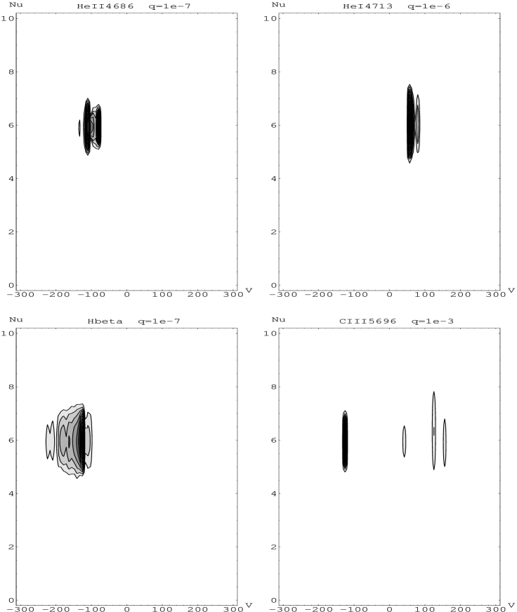
Figure 7 presents contour plots of the square of the amplitude of the Fourier transform (Fourier spectra) for the HeII$\,\lambda\,$4686, HeI$\,\lambda\,$4713, CIII$\,\lambda\,$5696 and CIII$\,\lambda\,$5696 lines. When constructing the density diagram for the power spectrum of the Fourier transformation, all values of the periodogram corresponding to low significance levels $q=10^{-7}-10^{-3}$ for the hypothesis that there was a strong white noise peak in the periodogram were rejected. Thus, only values corresponding to significances for the hypothesis that there is a harmonic component in the periodogram for a value $\alpha=1-q>0.999$ are presented in the plots.

Figure 7 has a broad peak at the frequency $\nu=5.9\pm 1\,d^{-1}$. The large width of the peak is due to the relatively low resolution of the Fourier spectrum, related to the short duration of the observations. The value $P=1/\nu\approx 4^{h}.1\pm 0^{h}.7$ exceeds the duration of the observations, and so cannot be directly identified with the period of the regular profile variations. We will call this value the quasi-period for the regular profile variations. Of course, the presence of regular line-profile variations with the proposed period must be confirmed by more extended observations. At present, we can only state that variations of the differential profiles in the spectrum of $\delta\,$Ori A are consistent with the period $\approx 4.1\pm 0.7^{h}$, with the same period being indicated for all the studied lines.

5 DISCUSSION

Our analysis shows that regular line profile variations with the characteristic time $P=4^{h}-6^{h}$ may occur in the spectrum of the $\delta\,$Ori A system. Such periods are typical for profile variations due to non-radial pulsations (NRPs) in O stars [4].

Apart from NRPs another possible origin for the rapid line profile variations is rotational modulation of the profiles. In the model of Kaper et al. [1], it is assumed that, along with a spherically symmetrical outflow in the form of a stellar wind, some denser, compact corotational streams rotating with the angular velocity of the star could be present in the atmosphere. It is proposed that additional absorption of the stellar radiation when these streams cross the line of sight results in regular line profile variations. The period of these variations will be $P_{n}=P_{rot}/n$, where $n$ is the number of corotational streams.

The orbital period $P_{rot}$ of the primary Aa¹ can be estimated from the data in the Table: $P_{\mbox{\scriptsize rot}}/\sin i\approx 3.6\,$d. The real inclination $i$ of the rotation axis of the primary is probably close to the orbit inclination, $67-77^{o}$ [14], which corresponds to $P_{rot}/sini\approx 3.6$ d. Explaining the quasi-period of the variations $P\approx 4^{h}.1$ as a result of rotational modulation of the profiles requires the value $n=21$, which does not seem plausible. In addition, in this case, we should see no fewer than 10 regular components in the entire line profile, which are not observed (Fig. 3).

Based on this reasoning, we conclude that the rotation of Aa¹ cannot give rise to the detected rapid profile variations with the quasi-period $P\approx 4^{h}.1$. Similar estimates based on data from the Table indicate that the rotation of Aa² and Ab likewise cannot explain the profile variations in the spectrum of $\delta\,$Ori A.

Thus, the most likely origin of the regular profile variations is photospheric NRPs of the stars in the $\delta\,$Ori A system. The relations $l\approx 0.1+1.09\mid\Delta\phi_{0}\mid/\pi$ and $m\approx\-1.33+0.54\mid\Delta\phi_{1}\mid/2pi$ can be used to determine the (l m) mode of the NRPs, where $\Delta\phi_{0}$ is the phase difference of the Fourier components of the line-profile variations of the main component $\nu_{0}$ of the NRPs and $\Delta\phi_{1}$ is the same value for its first harmonic $\nu_{1}=2\nu_{0}$ [30]. Unfortunately, due to the short duration of the data set $\Delta\phi_{0}$and $\Delta\phi_{1}$ cannot be determined with sufficient accuracy. The value $\Delta\phi_{0}$ for the H_β line profile can be determined only in the velocity interval $-18\div 150\,$km/s, and is equal to $\approx\pi$. Assuming that this value can be extrapolated to the entire velocity interval $\pm V\sin i$,we find $l\approx 2$.

Note that the profile variations of the studied lines in the spectrum of $\delta\,$Ori A are qualitatively similar to those in the spectra of numerous Be stars [38] that can be described as the result of NRPs in the sector mode $(l,\mid m\mid)=(2,2)$.

Let us now analyze the line profile variations in the spectrum of $\delta\,$Ori A supposing that they are related to NRPs in the $(2,\pm 2)$ mode. The velocity of a volume element of the star undergoing NRPs in spherical coordinates is $\propto Y_{ml}(\theta,\phi)exp(i\omega t)$, where $Y_{22}(\theta,\phi)\propto(1-\cos 2\theta)*exp(im\phi)$ is a spherical harmonic and $\omega$ is the angular frequency of the pulsations [30]. The time dependence of the velocity is specified by the factor $\exp(im\phi+\omega t)$, where $2\pi/\omega$ is the pulsation period. The phase velocity for the propagation of perturbations across the stellar surface is $\omega_{NRP}=2\pi*\omega/m$. This relation implies that the perturbation propagation period is twice the pulsation period.

The propagation of perturbations of the velocity of matter in the photosphere corresponds to movement of features in the differential profiles (peaks and valleys) with the same periods. This means that a profile feature associated with NRPs will cross the band $\pm V\sin i$ over for the time $T_{NRP}$, where $T_{NRP}$ is the NRP period. Therefore, we can write the approximate equality $T_{NRP}\approx T_{\mbox{\scriptsize{cross}}}$, where $T_{\mbox{\scriptsize{cross}}}$ is the time for the feature to cross the band $\pm V\sin i$ in the differential profile. We found the time $T_{\mbox{\scriptsize{cross}}}$ from our analysis of the wavelet spectra of differential profiles of the HeII$\lambda$4686 and HeI$\lambda$4713 photospheric lines (Fig. 5): $T_{\mbox{\scriptsize{cross}}}\approx 3-4^{h}$, very close to the quasi- period of the profile variations $P\approx 4^{h}$ determined above.

We conclude that the observed profile variations are consistent with the hypothesis that they are associated with photospheric NRPs of the primary, Aa¹, of the $\delta\,$Ori A system in the sector mode $(l,\mid m\mid)=(2,2)$. Since the profile features in the wavelet spectra move from the violet to the red part of the profile, $m<0$, yielding $(l,m)=(2,-2)$ for the NRP mode [30].

Apart from these features of the dynamical wavelet spectra, which we suppose to be related to NRPs, these spectra also display weaker features in the violet and red line wings beyond the $\pm V\sin i$ band. These cannot be due to variations in the photosphere of Aa¹. Two explanations for these specific features of the line profile variations are possible. First, they may be related to processes in the stellar wind in the expanding atmosphere of Aa¹. Since (i) we have estimated the contributions from Aa² and Ab to the main line profiles to be relatively small, (ii) CIIII$\,\lambda\,$5696 emission appears only in the spectra of the brightest hot supergiants (in our case, Aa¹), and (iii) the variability of the CIII emission is likely due to variability of photospheric absorption lines, and also exceeds the limits of the $\pm V\sin i$ band, we suggest that the variability of the main lines is primarily due to NRPs in the atmosphere of the Aa1 supergiant, and also to a variable contribution from the emission of the wind from the primary, modulated by its NRPs. Second, the variability beyond the $\pm V\sin i$ band could be related to the components Aa² and Ab.

Two clearly pronounced parallel structures are visible in the dynamical wavelet spectrum of the CIII$\,\lambda\,$5696 differential line profiles (Fig.5), associated with the movement of broad features in the wavelet spectrum towards negative velocities. The right component moves with a velocity of $\approx 180\,\mbox{km/s}$ to $\approx 40\,\mbox{km/s}$ and is located fully (taking into account its own line-profile widths) within the $\pm V\sin i$ band. The band crossing time for this component is $\approx 6^{h}$, which substantially exceeds the crossing time for the components of the HeII$\,\lambda\,$4686 and HeI$\,\lambda\,$4713 lines related to NRPs. These structures are undoubtedly associated with some imhomogeneities in the atmosphere that contribute to the emission at the CIII$\,\lambda\,$5696 line frequencies, rather than directly with NRPs of the primary. The possibility of generating quasi-regular structures in a stellar wind originating from photospheric NRPs is indicated in [37].

In support of this idea, we note that the patterns of the dynamical wavelet spectra related to gaseous imhomogeneities detected in the CIII emission, and also the wavelet spectrum features seen in other lines beyond the $\pm V\sin i$ band, are mutually complementary. Bringing into coincidence the wavelet spectra for the HeI$\lambda$4713 photospheric line and the CIII$\,\lambda\,$5696 envelope line (Fig. 5) indicates an avoidance of the wavelet spectra; i.e. the absence of any features in the CIII$\lambda$5696 emission wavelet spectrum in the velocity range containing the features in the HeI$\lambda$4713 photospheric absorption wavelet spectrum.

Figure 8: Position of components Aa¹ and Aa² (grey circles) in a diagram of $\log T_{\mbox{\scriptsize eff}}$ vs. pulsation period $P$ [39]. The top plot shows the periods for the pulsation modes $l=2$ for $\beta\,$Cep type stars and slowly pulsating B stars; the small dots indicate the calculated periods, and the bold dots the pulsation periods of main-sequence stars with masses of 5$M_{\odot}$ and 12$M_{\odot}$. The bottom plot shows the periods for pulsation modes $l=2$ for a main-sequence star with a mass of 30$M_{\odot}$.

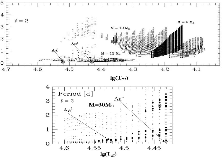
To clarify the extent to which the obtained quasi-period for the line-profile variations in the spectrum of $\delta\,$Ori A corresponds to possible pulsation periods of OB stars, we have plotted the positions of Aa¹ and Aa¹ on an diagram of effective temperature vs. pulsation period in the quadrupole mode $l=2$ for hot main-sequence stars ( [39], Figs. 6 and 7]. The positions of the components in Fig. 8 (top) are below the short-period boundary of the pulsation-instability strip for these stars, and do not correspond to the masses of the stars determined in[14] (see Table). At the same time, the position of Aa1 in the diagram calculated for a high-mass main-sequence star with M =30 M. (Fig. 8, bottom) accurately corresponds to the pulsation-instability strip for this star.

We suggest that, even in the case of substantial mass-loss from a star, its inner structure does not vary appreciably, and the periods of its NRPs correspond to pulsations for a main-sequence star whose mass is equal to the initial mass of the star up to the mass-loss stage.

Confirmation of the reality of the obtained period and clarification of the nature of the line-profile variations requires spectra of $\delta\,$Ori A obtained over two to three nights, making it possible to encompass four to six NRP cycles.

6 CONCLUSION

The following conclusions may be drawn from our observations.

1. All the studied lines display variable profiles, with the variability amplitude being 0.5%-1%. This conclusion has validity level of 0.999.

2. Large-scale components in the velocity interval 25-50 km/s are detected in the dynamical wavelet spectrum of the HeII$\,\lambda$4686, HeI$\,\lambda$4713,H., and CIII$\,\lambda$5696 line profile variations, which move in the $-V\sin i\div V\sin i$ band for the primary of the system, Aa¹, with a band crossing time of 4-5^h. Some variable features that go beyond the band are most likely due to emission imhomogeneities in the wind from $\delta\,$Ori Aa¹. The less bright components of the system Aa² or Ab may also contribute to the variability beyond the $-V\sin i\div V\sin i$ band. 3. We have found short-period variations of the studied line profiles with the characteristic times $\approx 4{{}^{h}}.1$.. We present evidence suggesting that these variations are associated with non-radial pulsations of the O9.5II primary of the system, Aa¹, in the sector mode $(l,m)=(2,-2)$.

7 ACKNOWLEDGEMENTS

The authors are grateful to V.E. Panchuk for assistance with the observations and to A.B. Schneiweiss for the Fourier spectra calculations. This work was supported by the Russian Foundation for Basic Research (project code 05-02-16995a), a Presidential Grant of the Russian Federation in Support of Leading Scientific Schools (NSh-088.2003.3), and a Presidential Grant of the Russian Federation in Support of Young Candidates of Science (MC- 874.2004.2). One of the authors (G.G.V.) acknowledges the Korea MOST Foundation (grant M1-0222-00-0005), as well as the KOFST and KASI programs (Brain Pool Program, Korea).

REFERENCES

- [1] Kaper L., Henrichs H.F., Fullerton A.W., Ando H. et al.// Astron. Astrophys., 1997. V. 327. P. 281.
- [2] Kaper L., Henrichs H.F., Nichols J.S., Telting J.H. et al., Astron. Astrophys. 1999. V. 344. P. 231.
- [3] Kaufer A., Stahl O., Wolf B. et al., Astron. Astrophys. 1996. V. 305. P. 887.
- [4] de Jong J.A., Henrichs H.F., Schrijvers S., Gies D.R., Telting J.H., Kaper L., Zwarthoed G.A. , Astron. Astroph. 1999. V. 345. P. 172.
- [5] Lépine S., Moffat A.F.J., Astrophys. J. 1999. V. 514. P. 909.
- [6] de Jong J.A., Henrichs H.F., Kaper L., Nichols J.S. et al., Astron. Astroph. 2001. V. 368. P. 601.
- [7] Kahn S.M., Leutenegger M.A., Cottam J. et al., Astron. Astrophys. 2001. V. 365, P. 365.
- [8] Miller N.A., Cassinelli J.P., MacFarlane J.J., Cohen D.H., Astroph. J. 2002. V. 499. P. L195.
- [9] Donati J.-F., Wade G.A., Babel J., Henrics H.F., de Jong J.A., HarriesT.J., Mothly Notices Roy. Astron. Soc. 2001. V. 326. P. 1265.
- [10] Donati J.-F., Babel J., Harries T.J., Howarth I.D., Petit P., Semel M., Mothly Notices Roy. Astron. Soc. 2002. V. 333. P. 55.
- [11] Neiner C., Hubert A.M., Floquet A.M., et. al., Astron. Astroph. 2002. V. 388. P. 899.
- [12] A. F. Kholtygin, D. N. Monin, A. E. Surkov, and S. N. Fabrika, Pis’ma Astron. Zh. 29, 208 (2003) [Astron. Lett. 29, 175 (2003)].
- [13] Hoffleit D., JAAVSO. 1996, V. 24. P. 105.
- [14] Harvin J.A., Gies D.R., Bagnuolo W.J., Jr., Penny L.R., Thaller M.R., Astroph. J., 2002. V. 565. P. 1216.
- [15] Maíz-Apelániz J. Walborn N.R., Astroph. J. Suppl Ser. 2004. V. 151. P. 103.
- [16] Voels S.A., Bohannan B., Abbot D.C., Hummer D.G., Astroph. J. 1989. V. 340. P. 1073.
- [17] Tarasov A.E. et al., Astron. and Astroph. Suppl. Ser. 1995. V. 110. P. 59.
- [18] Abt H.A., Levato H., Grosso M., Astroph. J., 2002. V.573 P. 359
- [19] Lamers H.J.G.L.M, Leitherer C. Astroph. J. 1993. V. 412. P. 771.
- [20] Wilson I.R.G., Dopita M.A., Astroph. J. 1985. V. 149. P. 295
- [21] Bieging J.H., Abbot D.C., Churcwell E.B., Astroph. J. 1989. V. 340, P. 518.
- [22] Grady C.A., Snow T.P., Cash W.C., Astroph. J. 1984. V. 283. P. 218.
- [23] Howarth I.D., Prinja R.K., , Astroph. J. Suppl. Ser. 1989. V. 69. P. 527
- [24] V. E. Panchuk, N. E. Piskunov, V. G. Klochkova, et al., Preprint No. 169, SAO (Special Astrophysical Observatory, Russian Academy of Sciences, Nizhnii Arkhyz, 2002).
- [25] V. E. Panchuk, V. G. Klochkova, and I. D. Naidenov, Preprint No. 179, SAO (Special Astrophysical Observatory, Russian Academy of Sciences, Nizhnii Arkhyz, 2003).
- [26] Ballester P., Astron. and Astroph. 1994. V. 286. P. 1011
- [27] Shergin V.S., Kniazev A.Yu., Lipovetsky V.A., Astron. Nachr. 1996. V. 317. P. 95.
- [28] D. Gray, The Observation and Analysis of Stellar Photospheres (Wiley, New York, 1976; Mir, Moscow, 1983).
- [29] Pierce A.K., Breckinridge J.B., Preprint KPNO. 1973. No. 1063.
- [30] Telting J.H., Schrijvers C., Astron. and Astroph. Suppl.Ser. 1997. V. 317. P. 723.
- [31] Fullerton A.W., Gies D.R. Bolton C.T., Astroph. J. Suppl. Ser. 1996. V. 103. P. 475.
- [32] S. Brandt, Statistical and Computational Methods in Data Analysis (North-Holland, Amsterdam, 1976; Mir, Moscow, 1975).
- [33] N. M. Astaf’eva,Usp.Fiz.Nauk 166, 1145 (1996) [Phys. Usp. 39, 1085 (1996)].
- [34] A. A. Koronovskii and A. E. Khramov, Nepreryvnyi veivletnyi analiz (Continuous Wavelet Analysis) (Fizmatlit, Moscow, 2003) [in Russian].
- [35] Roberts D.H., Lehar J., Dreher J.W., Astron. J. 1987. V. 93. P. 968.
- [36] V. V. Vityazev, Analiz neravnomernykh vremennykh ryadov (Analysis of Irregular Time Series) (St. Peterburg. Gos. Univ., St. Petersburg, 2001) [in Russian]
- [37] Owocki, S. P.; Cranmer, S. R., in Radial and Nonradial Pulsations as Probes of Stellar Physics, eds. C. Aerts, T.R. Bedding, J.Christensen-Dalsgaard,, ASP Conf. Proc., 259, 512 (1988)
- [38] Rivinius Th., Baade D., SteflS., Aston. Astroph. 2003. V. 411. P. 229.
- [39] Pamyatnykh A.A., Acta. Astron. 49, 189 (1999)