Candidate Milky Way Satellites in the Galactic Halo

Abstract

Aims. Sloan Digital Sky Survey (SDSS) DR5 photometric data with $120^{\circ}<\alpha<270^{\circ}$, $25^{\circ}<\delta<70^{\circ}$ are searched for new Milky Way companions or substructures in the Galactic halo.

Methods. Five candidates are identified as overdensities of faint stellar sources that have color-magnitude diagrams similar to those of known globular clusters or dwarf spheroidal galaxies. The distance to each candidate is estimated by fitting suitable stellar isochrones to the color- magnitude diagrams. Geometric properties and absolute magnitudes are roughly measured and used to determine whether the candidates are likely dwarf spheroidal galaxies, stellar clusters or tidal debris.

Results. SDSSJ1000+5730 and SDSSJ1329+2841 are likely faint dwarf galaxy candidates while SDSSJ0814+5105, SDSSJ0821+5608 and SDSSJ1058+2843 are likely extremely faint globular clusters.

Conclusions. Follow-up study is needed to confirm these candidates.

1 Introduction

The discovery of tidal streams in the Milky Way from the accretion of smaller galaxies supports hierarchical merging cosmogonies(Lynden-Bell & Lynden-Bell (1995)). The large-scale tidal arms of the Sagittarius dwarf spheroidal galaxy accretion event were the first to be discovered (Yanny et al. (2003); Majewski et al. (2003) and Rocha-Pinto et al. (2004)), and more tidal streams continue to be detected in Sloan Digital Sky Survey (SDSS; York et al. (2000)) data. The remarkably strong tidal tails of Palomar 5 are discovered by Odenkirchen et al. (2001), Rockosi et al. (2002) and Grillmair & Dionatos 2006a . Another tidal stream is connected with NGC5466 (Belokurov et al. 2006a ; Grillmair & Johnson (2006)). Belokurov et al. 2006b reveals the so-called Field of Streams, which shows not only Sagittarius arms but also the Virgo overdensity (Jurić et al. (2005)), Monoceros Ring (Newberg et al. (2002)), Orphan stream(Belokurov et al. 2006b ; Grillmair 2006a ) and a $60^{\circ}$-long stream between Ursa Major and Sextans (Grillmair & Dionatos 2006b ). The fact that tidal streams are often associated with globular clusters or dwarf spheroidal galaxies implies that it is possible to search for tidal streams by identifying new faint satellite dwarf galaxies, globular clusters or tidal debris and ascertaining their connections.

New satellite companions of the Milky Way have been discovered in the recent years. About 150 globular clusters (Harris (1996)) and 9 widely-accepted dwarf spheroidal galaxies (dSph) (Belokurov et al. (2007)) were known before the SDSS. Since 2005, tremendous progress has been made using SDSS data; at least nine new companions were discovered within two years. Seven of them are dSph satellites: Ursa Major I (Willman et al. 2005a ), Canes Venatici I(Zucker et al. 2006a ), Boötes (Belokurov et al. 2006c ), Ursa Major II (Zucker et al. 2006b ; Grillmair 2006a ), Coma Berenics, Canes Venatici II, Hercules and Leo IV (Belokurov et al. (2007)). Two of them are probably globular clusters: Willman 1 (Willman et al. 2005b ) and Segue 1 (Belokurov et al. (2007)).

It is impossible to see these objects in SDSS images since they are resolved into field stars. They are discovered by detecting local stellar overdensities in SDSS stellar databases (Belokurov et al. (2007)) by adding constraints on magnitude and color index. Overdensity study is a quick data mining method to find previously unknown satellite galaxies or globular clusters. We use a method similar to that of Belokurov et al. 2006c , but utilize different parameters, to scan an area of the sky bounded by $120^{\circ}<\alpha<270^{\circ}$, $25^{\circ}<\delta<70^{\circ}$, and observe five interesting overdensities with color-magnitude diagrams similar with a globular cluster or a dSph. They are candidate globular clusters or dSphs or tidal debris.

The organization of this paper is as follows. Section 2 describes our method of searching for candidates and how we measure their properties. Data acquisition and reduction processes, including the method for identifying candidates, are discussed in section 2.1. A template matching algorithm for estimating the distance to each overdensity is described in section 2.2. A rough measurement of geometric properties and radial profiles are addressed in section 2.3. In section 3 we discuss the nature of each overdensity. A short conclusion is included in the last session.

2 Discovery

2.1 Data Acquisition and Reduction

SDSS DR5 provides photometric data in $u$, $g$, $r$, $i$, and $z$ passbands (Fukugita et al. (1996)), and covers 8000 square degrees of sky (Adelman-McCarthy et al. (2007)). We select only the objects with stellar profiles from SDSS databases. SDSS recognizes all point sources as stars, including quasars and faint galaxies. Thus, galaxy clusters and arms and halos of bright galaxies contaminate our sample of overdensities. In order to decrease the frequency of these contaminants, we use only sources with magnitude $19<i<22$ and color $0<g-i<1$. We limited the area of sky searched to avoid the Sagittarius dwarf spheroidal galaxy’s tidal arms. Approximately $3.6\times 10^{7}$ point sources were obtained in the region $120^{\circ}<\alpha<270^{\circ}$, $25^{\circ}<\delta<70^{\circ}$ from SDSS Casjobs. The magnitudes in each band were corrected for extinction using values provided by the SDSS database, which are computed following Schlegel et al. (1998).

Data analysis procedures are based on the China Virtual Observatory’s experimental data access service(VO-DAS). We compute the star counts for this data in bins of size $0.2^{\circ}\times 0.2^{\circ}$ Hence, $750\times 225$ bins are generated. Field mean density and standard deviation for each bin are defined by the star counts in the surrounding bins, within a $11\times 11$ window. The standard deviation is derived from all bins in the box except the center bin. The strength of the peak in the center bin is estimated from:

$$\tilde{n}_{center}=(n_{center}-{\mu})/\sigma,$$ (1)

where $n_{center}$ is the number of stars in the center bin, $\mu$ is the average number of stars per bin in the surrounding bins, and $\sigma$ is the standard deviation. For most objects, the bin size is large enough to contain an entire star cluster; the surrounding bins contain many Galactic stars. For our sample, $\tilde{n}_{center}$ is normally distributed with $\tilde{\mu}=0.33$ and $\tilde{\sigma}=0.56$. We selected all peaks with $\tilde{n}_{center}>\bm{\tilde{\mu}+3\tilde{\sigma}\sim 2}$. From these statistics, we expect about $0.27\%$ of the bins we search will contain statistical fluctuations high enough to be detected as a peak. We searched 168750 bins, of which we excluded 18627 zero bins (sky areas which are not covered by SDSS). Therefore, we expect about 405 overdensities are actually caused by field star density fluctuation.

We actually identified 524 overdensity bins, which is 119 more than would be expected from statistics. The 524 overdensities include statistical fluctuations, previously identified Milky Way satellites, bright galaxies, bright stars, and galaxy clusters, in addition to the new Milky Way satellites we would like to find. We use additional information from the color-magnitude distribution of stars in the overdensities to cull out the statistical fluctuations, as described below. Known objects including bright galaxies, galaxy clusters, and bright stars are manually identified and eliminated. The known Milky Way satellites that were re-discovered by this technique include: UMa II, UMa I, Willman 1, Pal4, CVn II, CVn I, NGC5272, NGC5466, NGC6205, NGC6341, Draco, and Leo III, some of which cover more than 2 bins due to their large angular sizes. Overdensity bins which are close to the survey boundaries (within $0.5^{\circ}$) are also ignored.

Density contour diagrams and CMDs were generated within a $1^{\circ}\times 1^{\circ}$ area centered at the remaining overdensity bins. Candidates were manually identified by comparing the density contour diagram and CMD of each overdensities with those of 9 known objects: Pal 4, UMa I, UMa II, CVn I, Draco, NGC 6341, NGC 5466, Willman 1 and NGC 6205. The distance modulus (DM) of these templates ranges from 14.2mag to 21.7mag. This ensures that the templates cover all possible morphological features for a CMD, since the stellar populations that are probed within our magnitude limits depend on the distance modulus.

Five overdensities are finally chosen from over 500 initial candidates. Figure 1 displays density contours, core (circle with $r=0.1^{\circ}$ or $r=0.15^{\circ}$) CMDs, field (annuli area between $r=0.5^{\circ}$ and $r=0.6^{\circ}$) CMDs and Hess diagrams (subtraction between corresponding center area CMDs and field CMDs with normalized star counts) for these five candidate Milky Way satellites.

2.2 Distances to the Overdensities

Distances to the five candidates are estimated by fitting isochrone lines to the CMD of each overdensity. An automatic template-matching algorithm was developed to discover the best-fit Padova isochrone lines(Girardi et al. (2004)) for each candidate. Stellar evolution isochrone lines are converted to masks where the color index $g-i$ changes from -1 to 2 with step of 0.03 and the magnitude $i$ changes from -10 to 10 with step of 0.1. Thus a binary $100\times 200$ image mask for each isochrone line is formed. The value of each pixel in the image is either 1 (in the neighborhood of an isochrone line) or 0 (everywhere else). A series of mask templates are created for a range of metallicity, age and distance moduli. For each candidate, the template which minimizes $R$, as defined by the following formula, is selected as the best match.

$$R=\frac{\sum\limits_{g-i,i}{(C(g-i,i)(1-T(g-i,i,Z,A,DM)))}}{\sum\limits_{g-i,i}{C(g-i,i)}}$$ (2)

where $C(g-i,i)$ is the candidate’s Hess diagram ($i=13-22$mag). $T(g-i,i,Z,A,DM)$ is a template mask with specific metallicity $Z$, age $A$ and distance modulus $DM$. The value of $Z$ is 0.0001, 0.0004, 0.001, or 0.004. The value of $A$, in $log_{10}(yr)$, ranges from 9.5 to 10.25 with a step of 0.05. And the value of $DM$ ranges from 13mag to 21.9mag with a step of 0.1mag. In total 5760 templates were evaluated for each overdensity. The value of R also measures the goodness of the fit. The smaller R is, the better the fit.

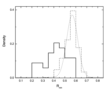
Figure 2: Comparison of $R_{min}$ for real objects compared with all original two sigma detections. Two populations of $R_{min}$ values distribution are displayed. The solid stair line shows all known objects, including globular clusters, dwarf galaxies, bright galaxies and galaxy clusters, and our five candidates. The distribution shows two peaks. The peak between 0.2 and 0.3 is due to 5 known globular clusters. The peak at 0.4 is associated with dwarf galaxies and normal galaxies. As comparison, the dashed stair line shows the distribution of all other overdensities with a gaussian fitting curve(dot line), where the average value is $R_{min}=0.57$ and $\sigma=0.1$. This figure shows that the globular clusters have the smallest $R_{min}$, the dwarf galaxies reach a larger radus, and both objects have a significantly smaller $R_{min}$ than non-candidates.

$R_{min}$, the minimum value of $R$, measures how many stars, in percent, are unrelated to the best fit isochrone line in the Hess diagrams. In the extreme case that stars are uniformly distributed in color-magnitude plane, considering that the isochrone line is only a thin line and cannot cover many stars in the plane, $R_{min}\sim 1$ is derived. In the opposite extreme case that the candidate contains no background stars so that its features are completely described by a template, $R_{min}\sim 0$ is reasonable. $R_{min}$ distributions for all known objects, candidates satellites and other overdensities are shown in Figure 2. The population of known objects and candidates addresses significantly smaller $R_{min}$ values than that of non-candidates overdensities.

Specifically, we use 9 known globular clusters and dwarf spheroidal galaxies: UMa I & II, CVn I & II, Pal4, NGC6205, NGC5466, NGC5272, and NGC6341, to test the effectiveness of the algorithm. They are all located in the detected area and were all detected by our selection process. Their distance moduli range from 14 to 22, as measured by previous authors (which are listed in Table 1). The standard deviation in the accuracy of the DM is $\sigma=0.23$mag.

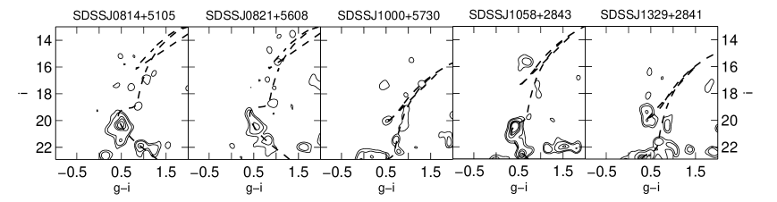
Figure 3: The Hess contours of candidates with the best-fitting isochrone lines overlaid on them. Contours are positive densities (0.05, 0.1, 0.15, 0.2, 0.25, 0.3 stars per bin). The size of each bin is $0.03mag\times 0.1mag$. Best-fitting stellar evolution isochrone lines are overlaid with dashed lines.

Best fit isochrone lines are shown together with Hess diagrams of our candidate Milky Way satellites in Figure 3. The distance modulus of the best fit template is an estimate of the distance to each overdensity. Table 2 displays the parameters of the matching templates for each candidates, though we don’t expect that this method of isochrone fitting will produce accurate measurements of the ages and metallicities of each candidate. We list our best fit metallicity and age parameters simply to show that they are not unreasonable for star clusters or dwarf galaxies in the Galactic halo.

$R_{min}$ values in table 1 again show the same trend with Figure 2 that globular clusters have smaller $R_{min}$ values, while low surface brightness dSphs (for example UMa II) have larger $R_{min}$ values. The fact that an acceptable DM is derived for UMa II, although it has a higher $R_{min}$ that reaches the non-candidates range(see Figure 2), gives us confidence that our technique for finding distances is valid even for these low surface brightness candidates.

2.3 Properties of Candidates

Center positions, geometric properties and absolute magnitudes are estimated for each candidate and listed in Table 2.

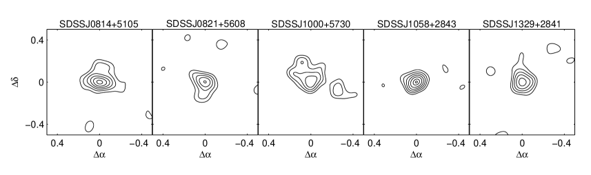
Figure 4: Isodensity contours of five candidates. The contour levels are 2, 3, 4, 5, 6, 7 and 7.5$\sigma$ above the background. The samples that generate the contours are selected from the corresponding Hess diagram.

In order to measure position and geometric properties for each candidate Milky Way satellite, stars associated with candidates are selected. We select stars which are located within the $1^{\circ}\times 1^{\circ}$ around the center position of candidates and also within bins in the Hess diagram (right panel in Figure 1) that have more than 0.05 stars per bin. Density contour diagrams of the five candidates are derived by counting selected stars and are displayed in Figure 4.

Because there are relatively few stars in our samples, we did not fit for the ellipticity of the candidates. We fit only circularly symmetric profiles. Background level is estimated by averaging star density of an annulus area around each candidates with radius from 30arcmin to 60arcmin. It is then subtracted from radial profile before fitting.

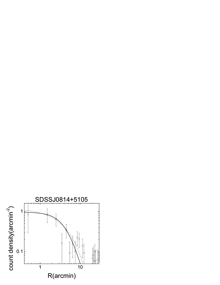
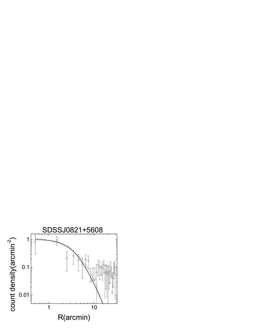
SDSSJ0821+5608

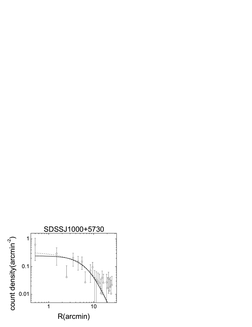
SDSSJ1000+5730

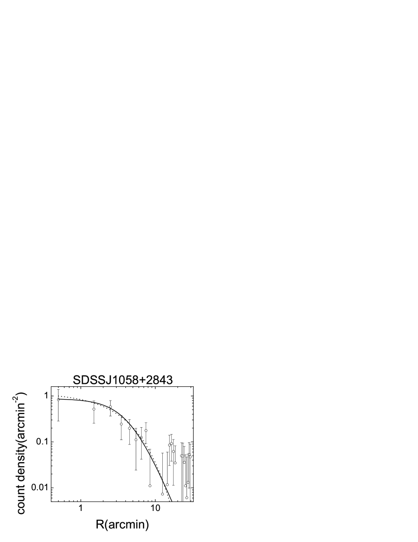
SDSSJ1058+2843

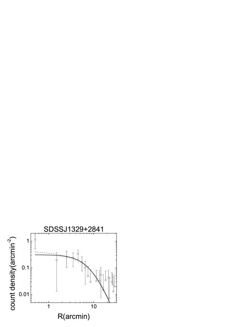
SDSSJ1329+2841

Figure 5: Density radial profiles for candidates.Background levels are subtracted before fitting models. The solid lines are Plummer model fit curves. The dashed lines are exponential model fit curves.

In order to check our methods, we compare the half-light radius of Pal5 and Boo using our method and compare the results with previous measurements in the literature. For Pal5 we derive $r_{h}=2.64^{\prime}\pm{0.07}$ for the exponential model and $r_{h}=2.91^{\prime}\pm{0.07}$ for the Plummer model. These values are similar to the previously measured value of $r_{h}=2.96^{\prime}$ in Harris (1996). For Boo, we find $r_{h}=14.4^{\prime}\pm{1.8}$ for the exponential model and $r_{h}=14.6^{\prime}\pm{1.5}$ for the Plummer model, while in Belokurov et al. 2006c corresponding values are $r_{h}=13.0^{\prime}\pm{0.7}$ and $r_{h}=12.6^{\prime}\pm{0.7}$. The results support our methods for estimating globular cluster and dwarf galaxy parameters, though there may be larger errors for lower luminosity objects. All candidates are fitted by exponential and Plummer models(McConnachie & Irwin (2006)). Radial profiles and fitting curves are displayed in Figure 5. Half-light radii derived by integrating exponential and Plummer profiles are tabulated in Table 2. Geometrical sizes of these candidates are computed from the estimated distances and the angular sizes from each model profile and also show in Table 2.

To estimate absolute magnitude of candidates we use Hess diagrams derived by subtracting field Hess diagrams from those generated by stars inside $\rm r_{h}$, normalized by area. Overlapping corresponding best matched isochrone masks on these Hess diagrams, only star counts located at neighbors of isochrone lines are kept. Then, g-band and r-band magnitudes are computed by integrating all positive flux values in these masked Hess diagrams. Total color index $\rm(B-V)_{tot}$ and Total apparent magnitude $\rm V{tot}$ are conducted from Formula 3 and 4 (Fukugita et al. (1996)).

$$(B-V)_{tot}=(g_{tot}-r_{tot}+0.23)/1.05$$ (3)

$$V_{tot}=r_{tot}+0.49(B-V)_{tot}-0.11$$ (4)

$$M_{V,tot}=V_{tot}+5-5log(d)$$ (5)

Consequently, absolute magnitudes are computed via 5. Absolute magnitudes estimated with different radial profile models are tabulated in Table 2. As a test, we estimate the absolute magnitudes of Com, CVn II, Her and Leo IV, which are low luminosity dwarf galaxies discovered in SDSS data(Belokurov et al. (2007)), using this method. The maximum bias of all four objects between our results and the literature’s is $\rm|\Delta M_{V,tot}|=0.55mag$, which is smaller than the standard error(0.6mag) mentioned in the literature. ANOVA analysis also shows that the estimation of our method is not significantly different with those from Belokurov et al. (2007).

3 Discussion

It is difficult to identify all 5 candidates reliably using only SDSS data; accurate follow up observations using a large telescope is required to determine the types, which could be: star clusters, dwarf spheroidal galaxies, tidal debris or chance superposition of field stars. We expect that these candidates are not merely field stars.

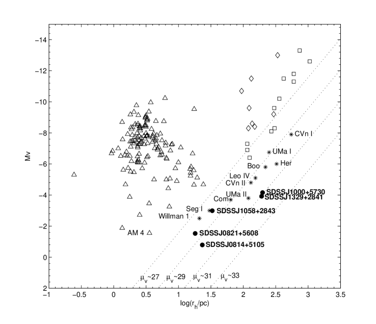
Figure 6: Location of different classes of objects in the plane of half light radius vs. absolute magnitude. Lines of constant surface brightness are marked. Filled circles with bold labels are the 5 candidates revealed in this paper. Triangles are known Globular Clusters (Harris (1996)). Stars with labels are Milky Way satellites discovered from SDSS(Belokurov et al. 2006c , Belokurov et al. (2007), Zucker et al. 2006b , Willman et al. 2005a and Willman et al. 2005b ), Diamonds are dwarf galaxies in the local group(Irwan & Hatzidimitriou (1995) and Mateo (1998)). Rectangles are Andromeda dwarf galaxies(McConnachie & Irwin (2006) and Martin et al. (2006))

Belokurov et al. (2007) uses the $R_{h}$ vs. $M_{V}$ plane to identify Her, Leo IV, CVn II, Com as dSphs, while Seg I is an unusual low luminosity globular cluster. We adopt that same method, and plot our candidates with known Milky Way satellites in Figure 6. The half-light radii of 5 candidates are derived by integrating exponential profiles and Plummer profiles. The absolute magnitudes are derived by adding all possible member stars flux which located in half-light radius and time 2. We plot the 5 candidates in $R_{h}$ vs. $M_{V}$ plane with the mean values derived by exponential and Plummer model. $R_{h}$ and $M_{V}$ of known globular clusters are come from Harris (1996), and those of SDSS discovered Milky Way dwarf spheroidal galaxies are come from Belokurov et al. 2006c , Belokurov et al. (2007), Zucker et al. 2006b , Willman et al. 2005a and Willman et al. 2005b , those of dwarf galaxies in the local group are come from Irwan & Hatzidimitriou (1995) and Mateo (1998), and those of Andromeda dwarf galaxies are come from McConnachie & Irwin (2006) and Martin et al. (2006).

SDSSJ0814+5105, SDSSJ0821+5608 and SDSSJ1058+2843:

SDSSJ0814+5105, SDSSJ0821+5608 and SDSSJ1058+2843 have surface brightness which are similar to other known satellites discovered from SDSS with extremely faint absolute magnitudes, even fainter than AM4, the faintest one in Harris (1996). Their location in Figure 6 suggests that these stellar systems are more similar to globular clusters than to dwarf galaxies. Tidal radii of SDSSJ0814+5105 , SDSSJ0821+5608 and SDSSJ1058+2843 in Figure 6 are computed using the equation

$$r_{tidal}\sim{R(\frac{M_{cand}}{3M_{MW}})^{1/3}}$$ (6)

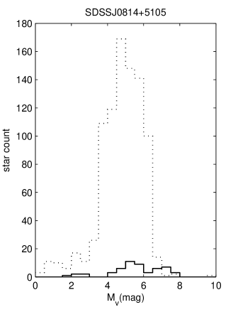
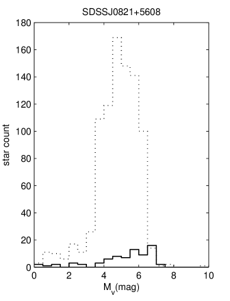
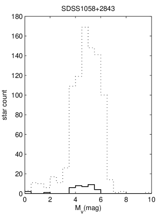
Figure 7: Luminosity function comparison between SDSSJ0814+5105, SDSSJ0821+5608 and SDSSJ1058+2843, marked as solid line, and Pal 5, marked as dot line, within half-light radii. Stars between 4 and 6 mag correspond to spectral types from F to G in main sequence. Star counts of F and G stars are used to roughly estimate the total mass.

from Binney & Tremaine (1987), where $R$ is the candidate’s galactocentric distance, $M_{cand}$ is its total mass, and $M_{MW}$ is the total mass of the Milky Way within $R$. We assume that the distance from the Sun to the center of the Milky Way is 8kpc and $v_{c}=220kms^{-1}$ at distance $R$. $M_{cand}$ is estimated by comparing star counts of F and G stars located in main sequences of the three candidates and Pal 5 (Figure 7). Since the formula for the tidal radius does not include dark matter, the actual tidal radius is larger than estimated if the candidates are dwarf galaxies with substantial dark matter content.

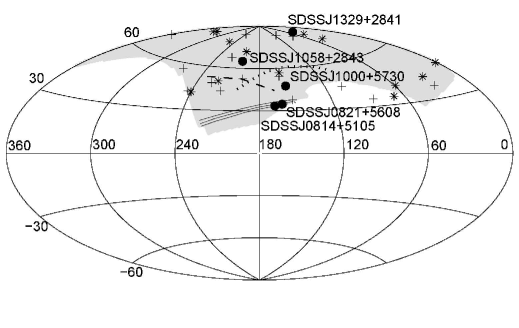
Figure 8: Overdensities’ positions in galactic coordinates in Aitoff projection. The gray area encloses the main area of North Galactic Cap covered by the SDSS DR5 data. Filled circles are candidates in this paper. Plus symbols are UMa II, Willman 1, UMa I, CVn I, CVn II, Her, Leo IV, Com and Seg 1. Star symbols are globular clusters in the SDSS DR5 area we detect. The triple thin solid lines are Anticenter Stream of Grillmair 2006b which may be related to the Monoceros Ring. The thin dotted line is GD-1. The thin dashed line is Orphan stream.

Notice that SDSSJ0814+5105 and SDSSJ0821+5608 overlap the Anticenter Stream (Grillmair 2006b ), which may be related to Monoceros Ring displayed in Figure 8. According to Newberg et al. (2002) the turnoff magnitude of Monoceros Ring is at $g=19.4$. In Figure 1 we estimate SDSSJ0814+5105 and SDSSJ0821+5608 has a magnitude of the turnoff as $g=19.5$. They are almost at the same distance. However, according to Grillmair 2006b , the Anticenter Stream has a turnoff magnitude as $g=18.7$, quite different from the results of Newberg et al. (2002) and substantially closer than the new candidates. The question is, are they globular clusters in the Monoceros stream, or are they just part of the debris more compact than in other areas?

SDSSJ1000+5730 & SDSSJ1329+2841: SDSSJ1000+5730 and SDSSJ1329+2841 are faint, extended objects with half light radii similar to that of most of dSphs. They have surface brightness near $\mu_{V}\sim{31}mag/arcsec^{2}$, which are lower than all known dSphs discovered from SDSS. Their type cannot be determined only by SDSS due to their faintness, but they look like dwarf galaxies.

4 Conclusions

In this paper we report five interesting overdensities detected in the SDSS database. They show features of globular clusters or dSphs in their CMDs. Mass estimation for SDSSJ0814+5105, SDSSJ0821+5608 and SDSSJ1058+2843 indicate that their tidal radii are bigger than their half-light radius, which implies that they are likely globular clusters with low surface brightness. The half-light radius and absolute magnitude of SDSSJ1329+2841 suggest a likely dSph. Although surface magnitude measurements suggest that SDSSJ1000+5730 is fainter than all known dSphs, its Hess diagram implies that it is an interesting object that needs follow-up observations.

H.N. acknowledges funding from the National Science foundation (AST 07-33161).

Funding for the SDSS and SDSS-II has been provided by the Alfred P. Sloan Foundation, the Participating Institutions, the National Science Foundation, the U.S. Department of Energy, the National Aeronautics and Space Administration, the Japanese Monbukagakusho, the Max Planck Society, and the Higher Education Funding Council for England. The SDSS Web Site is http://www.sdss.org/.

The SDSS is managed by the Astrophysical Research Consortium for the Participating Institutions. The Participating Institutions are the American Museum of Natural History, Astrophysical Institute Potsdam, University of Basel, University of Cambridge, Case Western Reserve University, University of Chicago, Drexel University, Fermilab, the Institute for Advanced Study, the Japan Participation Group, Johns Hopkins University, the Joint Institute for Nuclear Astrophysics, the Kavli Institute for Particle Astrophysics and Cosmology, the Korean Scientist Group, the Chinese Academy of Sciences (LAMOST), Los Alamos National Laboratory, the Max-Planck-Institute for Astronomy (MPIA), the Max-Planck-Institute for Astrophysics (MPA), New Mexico State University, Ohio State University, University of Pittsburgh, University of Portsmouth, Princeton University, the United States Naval Observatory, and the University of Washington.

Table 1: Comparison of distances from template matching method with previous studies

Name	Z from template	Age from template	DM from template	DM from references	$R_{min}$	References
		($log_{10}(yr)$)	(mag)	(mag)
UMa II	0.0004	10.1	17.9	17.5	0.50	Zucker et al. 2006b
UMa I	0.0001	10	19.9	20	0.41	Willman et al. 2005a
Pal4	0.001	10.2	20.2	20.02	0.37	Harris (1996)
CVn II	0.0004	10.2	20.9	20.9	0.25	Belokurov et al. (2007)
CVn I	0.0004	10.15	21.7	21.75	0.28	Zucker et al. 2006a
NGC5272	0.001	10.1	15	15.04	0.21	Harris (1996)
NGC5466	0.001	10.05	16.1	16.1	0.34	Harris (1996)
NGC6205	0.004	9.95	14.7	14.28	0.21	Harris (1996)
NGC6341	0.001	10	14.9	14.59	0.28	Harris (1996)

Table 2: Parameters of each overdensity.

Parameter	SDSSJ0814+5105	SDSSJ0821+5608	SDSSJ1000+5730	SDSSJ1058+2843	SDSSJ1329+2841
RA(J2000)	$\rm 08^{h}13^{m}42^{s}$	$\rm 08^{h}21^{m}15^{s}$	$\rm 10^{h}00^{m}28^{s}$	$\rm 10^{h}58^{m}04^{s}$	$\rm 13^{h}29^{m}13^{s}$
DEC(J2000)	$\rm+51^{\circ}05^{\prime}27^{\prime\prime}$	$\rm+56^{\circ}08^{\prime}16^{\prime\prime}$	$\rm+57^{\circ}30^{\prime}10^{\prime\prime}$	$\rm+28^{\circ}42^{\prime}39^{\prime\prime}$	$\rm+28^{\circ}41^{\prime}27^{\prime\prime}$
l(deg)	167.743	161.665	155.506	202.649	45.716
b(deg)	33.449	34.615	47.372	64.966	81.513
Z	0.004	0.004	0.001	0.004	0.0004
Age($\rm log_{10}(yr)$)	10.5	10	10.15	9.95	10.1
$\rm(m-M)_{0}$(mag)	15.7	15.7	19.6	16.9	19.4
$\rm R_{min}$	0.5	0.45	0.47	0.36	0.58
Distance(kpc)	$13.8^{+1.5}_{-1.4}$	$13.8^{+1.5}_{-1.4}$	$83.2^{+9.3}_{-8.4}$	$24^{+2.7}_{-2.4}$	$75.9^{+8.5}_{-7.6}$
$\rm r_{h}$(exponential)(arcmin)	$\rm 6.2\pm{1.0}$	$\rm 4.7\pm{1.0}$	$\rm 8.1\pm{2.7}$	$\rm 4.7\pm{0.7}$	$\rm 8.6\pm{2.5}$
$\rm r_{h}$(Plummer)(arcmin)	$\rm 5.4\pm{0.8}$	$\rm 4.3\pm{0.8}$	$\rm 8.3\pm{2.2}$	$\rm 4.8\pm{0.5}$	$\rm 8.8\pm{1.9}$
$\rm r_{h,g}$(exponential)(pc)	$\rm 24.9\pm{4.0}$	$\rm 18.9\pm{4.0}$	$\rm 196.0\pm{63}$	$\rm 32.8\pm{4.9}$	$\rm 189.8\pm{55}$
$\rm r_{h,g}$(Plummer)(pc)	$\rm 21.7\pm{3.2}$	$\rm 17.3\pm{3.2}$	$\rm 200.8\pm{53}$	$\rm 33.5\pm{3.5}$	$\rm 194.2\pm{42}$
Background level($\rm arcmin^{-2}$)	0.11	0.1	0.02	0.12	0.12
$\rm M_{V}$(exponential)(mag)	-0.77	-1.63	-4.15	-2.99	-3.91
$\rm M_{V}$(Plummer)(mag)	-0.81	-1.42	-4.16	-2.98	-3.92

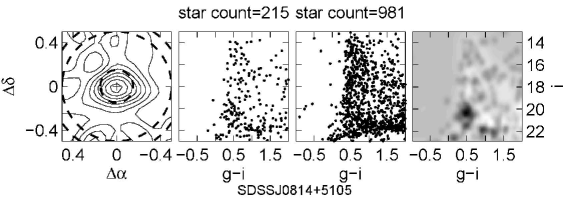
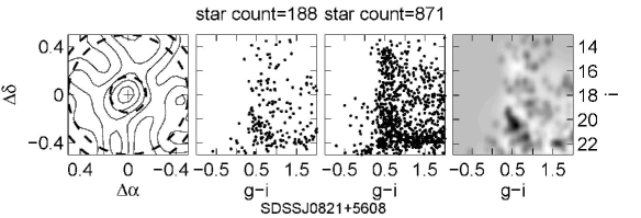
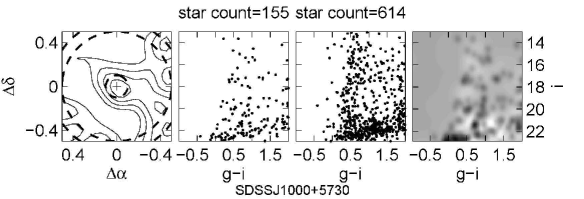
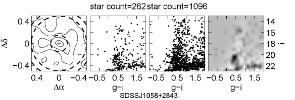
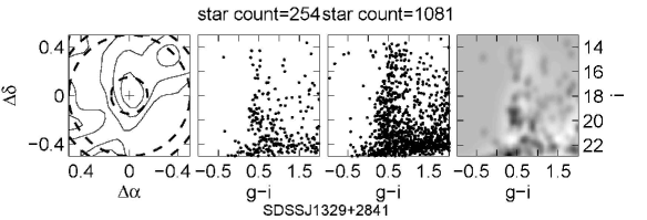
Figure 1: Overdensity detections. The first column of diagrams are density contours. Each density contour is constructed by nonparametric distribution density estimation with a Gaussian kernel and a window width of $0.1^{\circ}$, using stars with $19<i<22$mag located in the $1^{\circ}\times 1^{\circ}$ area around the candidate. The second column of diagrams displays the core CMDs of overdensities. Points in this column are samples from the smallest circle ($r=0.1^{\circ}$ or $0.15^{\circ}$) overlaid on density contours. The third column of diagrams displays field CMDs of the overdensities. Points in this column are samples from the annuli between the intermediate circle ($r=0.5^{\circ}$) and the biggest circle ($r=0.6^{\circ}$). The right most column of diagrams are Hess diagrams which are the result of subtraction between the core CMDs and corresponding field CMDs with normalization on total star counts. The size of each bin in the Hess diagrams is $0.03mag\times 0.1mag$.

References

- Adelman-McCarthy et al. (2007) Adelman-McCarthy, J., et al., 2007, ApJS, submitted
- Binney & Tremaine (1987) Binney, J., & Tremaine, S., 1987, Galactic Dynamics (Princeton: Princeton Univ. Press)
- Cox (2000) Cox, A. N. ed., 2000, Allen’s Astrophysical Quantities (4th edition), Springer-Verlag New York Inc., p.400
- (4) Belokurov L., et al., 2006a, ApJ, 637, L29
- (5) Belokurov L., et al., 2006b, ApJ, 642, L137
- (6) Belokurov L., et al., 2006c, ApJ, 647, L111
- Belokurov et al. (2007) Belokurov L., et al., 2007, ApJ, 654, 897
- Bergbusch & VandenBerg (1992) Bergbusch, P. S., & VandenBerg, D. A., 1992, ApJS, 81, 163
- Fukugita et al. (1996) Fukugita, M., et al., 1996, AJ, 111, 1748
- Fellhauer et al. (2006) Fellhauer, M., et al., 2006, MNRAS, submitted astro-ph/0611157
- Grillmair & Smith (2001) Grillmair, C. J., & Smith, G. H., AJ, 122, 3231
- (12) Grillmair, C. J., & Dionatos, O. 2006a, ApJ, 641, L37
- (13) Grillmair, C. J., & Dionatos, O. 2006b, ApJ, 643, L17
- Grillmair & Johnson (2006) Grillmair, C. J., & Johnson, R. 2006, ApJ, 639, L17
- (15) Grillmair, C. J., 2006a ApJ, 645, L37
- (16) Grillmair, C. J., 2006b ApJ, 651, L29
- Girardi et al. (2004) Girardi L.,et al., 2004 A&A, 422, 205
- Harris (1996) Harris, W. E., 1996, AJ, 112, 1487
- Irwan & Hatzidimitriou (1995) Irwin, M., & Hatzidimitriou, D., 1995, MNRAS, 277, 1354
- Jurić et al. (2005) Jurić, M., et al., 2005 ApJ, submitted astro-ph/0510520
- King (1962) King, I., 1962, AJ, 67, 471
- Lee, Demarque & Zinn (1990) Lee, Y.-W., Demarque, P., Zinn, R., 1990, ApJ, 350, 155
- Lynden-Bell & Lynden-Bell (1995) Lynden-Bell, D., & Lynden-Bell, R. M., 1995, MNRAS, 275, 429
- Majewski et al. (2003) Majewski, S. R., et al., 2003, ApJ, 599, 1082
- Mandushev et al. (1991) Mandushev, G., Spassova, N., & Staneva, A., 1991, A&A, 252, 94
- Martin et al. (2006) Martin, N., et al., 2006 MNRAS, 371, 1983
- Mateo (1998) Mateo, M. L., 1998, ARA&A, 36, 435
- McConnachie & Irwin (2006) McConnachie, A. W., & Irwin, M. J., 2006, MNRAS, 365, 1263
- Newberg et al. (2002) Newberg, H. J., et al. 2002, ApJ, 569, 245
- Odenkirchen et al. (2001) Odenkirchen, M., et al. 2001, ApJ, 548, L165
- Rocha-Pinto et al. (2004) Rocha-Pinto, et al., 2004, ApJ, 615, 732
- Rockosi et al. (2002) Rockosi, C. M., et al. 2002, AJ, 124, 349
- Schlegel et al. (1998) Schlegel, D. J., Finkbeiner, D. P., & Davix, M., 1998 ApJ, 500, 525
- Stetson et al. (1999) Stetson, P. B., et al., 1999, AJ, 117, 247
- (35) Willman, B., et al., ApJ, 626, L85
- (36) Willman, B., et al., AJ, 129, 2692
- Yanny et al. (2003) Yanny, B., et al., 2003, ApJ, 588, 824
- York et al. (2000) York, D. G., et al., 2000 AJ, 120, 1579
- Zucker et al. (2004) Zucker, D. B., et al., 2004 ApJ, 612, L121
- (40) Zucker, D. B., et al., 2006a ApJ, 643, L103
- (41) Zucker, D. B., et al., 2006b ApJ, 650, L41