The extended star formation history of the star cluster NGC 2154 in the Large Magellanic Cloud

Abstract

The color-magnitude diagram (CMD) of the intermediate-age Large Magellanic Cloud (LMC) star cluster NGC 2154 and its adjacent field, has been analyzed using Padova stellar models to determine the cluster’s fundamental parameters and its Star Formation History (SFH). Deep $BR$ CCD photometry, together with synthetic CMDs and Integrated Luminosity Functions (ILFs), has allowed us to infer that the cluster experienced an extended star formation period of about 1.2 Gyrs, which began approximately 2.3 Gyr and ended 1.1 Gyr ago. The physical reality of such a prolonged period of star formation is however questionable, and could be the result of inadequacies in the stellar evolutionary tracks themselves. A substantial fraction of binaries (70$\%$) seems to exist in NGC 2154.

The star cluster NGC 2154

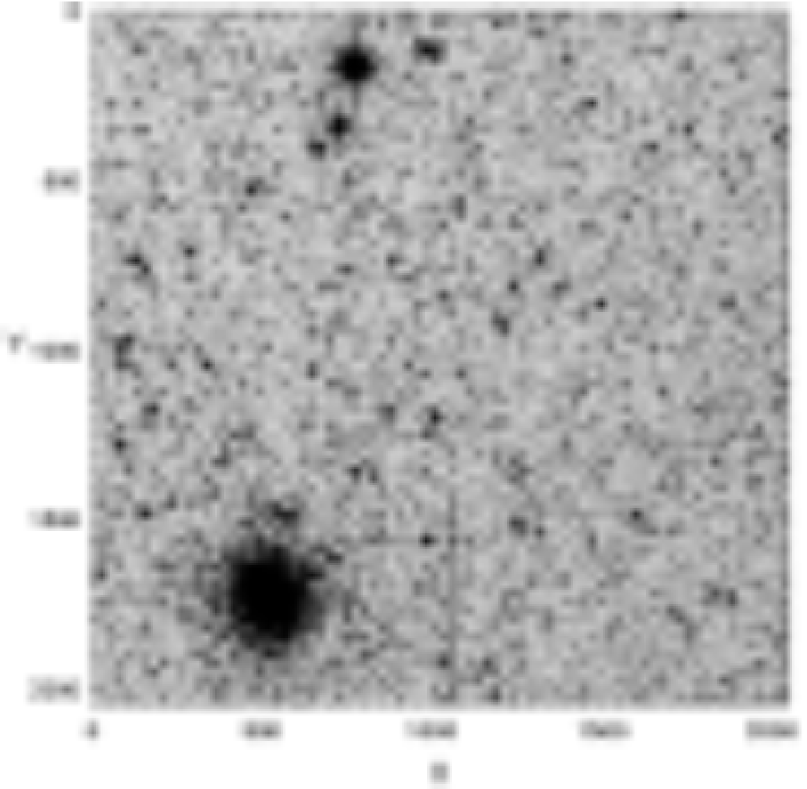
Figure 1: $R$ band image of NGC 2154 and the adjacent LMC stellar field. North is up, East to the left. The size of the field is $8\aas@@fstack{\prime}85\times 8\aas@@fstack{\prime}85$

1 Introduction

The star cluster system of the Magellanic Clouds (MCs) differs significantly from that of the Milky Way (and also from one another), differences which are commonly attributed to a different chemical and dynamical evolution. Furthermore, MC clusters exhibit a broad range of properties in contrast to our galaxy, thus representing a more ample range of stellar populations than those represented by Galactic clusters. For the above reasons, MCs clusters have become a challenging domain for stellar and galactic evolutionary models, and are routinely used as an observational workbench to address these issues (see e.g. Barmina et al. 2002, Bertelli et al. 2003, Woo et al. 2003). A very specific case is that of the intermediate-age, metal-poor populations, which are conspicuous in the MC, yet rather poorly represented in our galaxy.

One of many examples of intermediate-age clusters in the LMC is NGC 2154. Although this cluster is morphologically globular, it is considered to be of intermediate age (SMB type V; Searle et al. 1980). Persson et al. (1983) were able to constrain its age to the 1-3 Gyr range, but a detailed study of its basic parameters (requiring high-precision deep photometry) was still lacking.

Here we present deep CCD photometry, reaching B,R$\sim$25, of NGC 2154 and its adjacent LMC field, which has allowed for an unprecedented study of the cluster, and a first-ever study of the SFH of this LMC field. The present work is one result of a more comprehensive study of the MCs, which includes the study of their SFH (Noel et al. 2006; submitted to AJ), and the determination of their absolute proper motions with respect to background QSOs (see e.g. Pedreros et al. 2006). One of the LMC QSO fields selected for the proper-motion work by chance included the neglected LMC cluster NGC 2154, which gave us the possibility to observe this cluster -and its surrounding field- routinely during our four-year (2001-4) campaign, with the (additional) motivation of determining not only its fundamental parameters, but also the SFH of the field (which will be the subject of a forthcoming paper; Girardi et al. 2007).

The layout of the paper is as follows. Sect. 2 and 3 describe the observations and the reduction strategy. In Sect. 4 we study the cluster structure and derive an estimate of its radius. Sect. 5 and 6 deal with the CMDs and describe the derivation of the cluster fundamental parameters. In Sect. 7 we summarize our conclusions.

2 Observations

$B(R)_{KC}$ images of the NGC 2154 region in the LMC were acquired with a 24$\mu$ pixels Tektronix 2048$\times$2048 detector attached to the Cassegrain focus of the du Pont 2.5-meter telescope (C100) at Las Campanas Observatory, Chile. Gain and read noise were 3 e-/ADU and 7 e-, respectively. This set-up provides direct imaging over a field of $8\aas@@fstack{\prime}85\times 8\aas@@fstack{\prime}85$ with a scale of $0\aas@@fstack{\prime\prime}259$/pix. This relatively large field of view allowed us to include the cluster and a good sampling of the LMC field in all frames. The field covered by the observations is shown in Fig. 1.

Details on the available frames and their corresponding exposure times are listed in Table 1. The B and R band-passes were selected in order to satisfy both the needs of the SFH and astrometry programs (for this latter it was mandatory to obtain R-band images). Typical seeing was about $0\aas@@fstack{\prime\prime}9$.

All frames were pre-processed in a standard way using the IRAF package CCDRED. For this purpose, zero exposures and sky flats were taken every night.

Table 1: Log-book of observations for NGC 2154.

Date	Airmass	Filter	Exp. Time
			[sec.$\times$	N]
15-10-01	1.28	$R$	60$\times$	1
	1.28	$R$	300$\times$	3
16-10-01	1.27	$R$	400$\times$	3
17-10-01	1.28	$B$	400$\times$	1
	1.27	$R$	400$\times$	3
18-10-01	1.28	$R$	400$\times$	3
08-10-02	1.51	$R$	60$\times$	1
	1.49	$R$	400$\times$	9
	1.30	$B$	400$\times$	1
	1.29	$B$	600$\times$	4
09-10-02	1.51	$R$	60$\times$	2
	1.31	$B$	60$\times$	1
	1.30	$B$	600$\times$	1
	1.28	$R$	300$\times$	3
	1.28	$R$	400$\times$	1
10-10-02	1.29	$B$	60$\times$	1
	1.29	$B$	600$\times$	1
	1.28	$R$	400$\times$	1
11-10-02	1.37	$B$	60$\times$	1
	1.32	$B$	600$\times$	4
	1.30	$R$	400$\times$	2
	1.28	$R$	300$\times$	4
12-10-02	1.37	$B$	60$\times$	1
	1.37	$B$	600$\times$	3
	1.28	$R$	60$\times$	1
	1.28	$R$	300$\times$	3
20-10-03	1.29	$R$	60$\times$	1
	1.29	$R$	200$\times$	4
	1.27	$B$	800$\times$	3
21-10-03	1.29	$R$	60$\times$	1
	1.29	$B$	800$\times$	3
	1.28	$R$	300$\times$	4
22-10-03	1.29	$R$	600$\times$	1
	1.27	$R$	300$\times$	4
24-10-03	1.31	$R$	60$\times$	1
	1.31	$R$	600$\times$	2
	1.29	$R$	300$\times$	6
04-11-04	1.30	$R$	60$\times$	1
	1.29	$R$	600$\times$	6
	1.28	$B$	800$\times$	3
05-11-04	1.31	$R$	5$\times$	3
	1.30	$R$	30$\times$	3
	1.30	$R$	300$\times$	2
	1.29	$B$	10$\times$	4
	1.28	$B$	120$\times$	3
	1.28	$B$	600$\times$	2
	1.27	$R$	60$\times$	2
	1.27	$R$	300$\times$	5
	1.27	$B$	600$\times$	6

$N$ indicates the number of frames obtained.

Table 2: Coefficients of the calibration equations

	run 2001
	(four nights)
$b_{1}$	$+0.734\pm 0.003$
$b_{2}$	$+0.218\pm 0.002$
$b_{3}$	$-0.044\pm 0.001$
$r_{1}$	$+0.434\pm 0.003$
$r_{2}$	$+0.083\pm 0.002$
$r_{3}$	$-0.001\pm 0.001$

3 The Photometry

3.1 Standard star photometry

Our instrumental photometric system was defined by the use of the Harris UBVRI filter set, which constitutes the default option at the C100 for broad-band photometry on the standard Johnson-Kron-Cousins system. On photometric nights, standard star areas from the catalog of Landolt (1992) were observed multiple times to determine the transformation equations relating our instrumental (b, r) magnitudes to the standard (B, R_KC) system. To determine atmospheric extinction optimally, a few of them were followed each night up to about 2.0 air-masses. Besides, the standard star fields were selected to provide a wide color coverage, being $-0.4\leq(B-R)\leq 3.6$ (see Fig. 2). Aperture photometry was carried out for all the standard stars using the IRAF DAOPHOT/PHOTCAL package.

To put our observations into the standard system, we used transformation equations of the form:

$b=B+b1+b2*X+b3*(B-R)$
$r=R+r1+r2*X+r3*(B-R)$

In these equations $b$, $r$ are the aperture magnitude already normalized to 1 sec, and $X$ is the airmass. We did not include second-order color terms because they turned out to be negligible in comparison to their uncertainties. The values of the transformation coefficients are listed in Table 2. The night-to-night variation of the coefficients turned out to be very small ($\sim$ 0.001), so we adopted the average values over all nights. The residuals resulting from the fits are showed in Fig. 2, and the global rms of the calibration was 0.011 mag for both B and R filters.

3.2 Cluster and LMC field photometry

Here we follow the procedure outlined in Baume et al. (2004). We first averaged images taken the same night, and with the same exposure time and filter, in order to get a higher signal-to-noise ratio for the faint stars, and also to clean the images from cosmic rays. Then, instrumental magnitudes and (X,Y) centroids of all stars in each frame were derived by means of profile-fitting photometry with the DAOPHOT package, using the Point Spread Function (PSF) method (Stetson 1987); and all instrumental magnitudes from different nights were combined and carried to same system (2001 reference) by using DAOMASTER (Stetson 1992). Stellar magnitudes in the standard system were obtained then by using the transformations indicated in section 3.1.
This resulted in a photometric catalog consisting of about 20000 stars

In Fig. 3 we present the photometric errors trends (from DAOPHOT and DAOMASTER) as a function of the B magnitude. Down to $B=22$, both the $B$ band and $R$ band errors remain lower than 0.025 mag. From Fig. 2 it can be easily seen that the main source of error originates in the B-band observations. It is this filter that determines the deepness of our photometry, a point that is relevant to the completeness analysis (see Sect. 3.3).

3.3 Photometric completeness

For all comparisons described in the next sections, completeness of the observed star counts is a relevant issue. Completeness corrections were determined by means of artificial-star experiments on our data (see Carraro et al. 2005). Basically, we created several artificial images by adding in random positions a total of 40000 artificial stars to our true images. They were distributed with a uniform probability distribution with the same color and luminosity of the real sample . In order to avoid the creation of overcrowding, in each experiment we added the equivalent to only 15of the original number of stars.

Given that in general the $B$ band images are shallower than those in the $R$ band, we have adopted as completeness factor that estimated for $B$. This factor is defined as the ratio between the number of artificial stars recovered and the number of artificial stars added. Computed values of the completeness factor for different B magnitude bins are listed in Table 3, both for the cluster (r ¡ 400 pix), and for a representative comparison field (see Sect. 6.1). It must be noticed that due to the inherent nature of a very compact star cluster (see Figs. 1 and 4), more than half of the stars would occupy less than half of the volume. As a consequence, the completeness fractions for the cluster stars are likely to be a bit overestimated. On the other hand, the use of a lower radius for the cluster region would have the disadvantage to imply larger uncertainties in the completeness factors.

Table 3: Completeness analysis results in the $B$ band.

$\Delta B$	NGC 2154	Field
	(r$<$400pix)
19.5-20.0	100.0%	100.0%
20.0-20.5	92.7%	100.0%
20.5-21.0	75.1%	100.0%
21.0-21.5	57.4%	100.0%
21.5-22.0	56.8%	100.0%
22.0-22.5	56.1%	100.0%
22.5-23.0	55.0%	100.0%
23.0-23.5	53.9%	82.7%
23.5-24.0	41.7%	61.1%
24.0-24.5	29.5%	62.0%
24.5-25.0	32.4%	65.6%
25.0-25.5	35.2%	82.5%
25.5-26.0	36.3%	49.6%

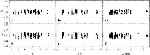
Figure 2: Trend of residuals of the standard stars calibration.

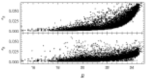
Figure 3: Photometric errors in $B$ and $R$ given by DAOPHOT and DAOMASTER, as a function of the $B$ magnitude.

4 Star counts

4.1 Cluster radius

In order to study the cluster structure, as a first step we estimated the position of the cluster center by determining the highest peak in the stellar density, which was done by visual inspection of the our images. This peak was found at: $X=515$; $Y=1725$, which corresponds to $\alpha_{2000}=5^{h}57^{m}38^{s}.2$; $\delta_{2000}=-67^{o}15^{\prime}40^{\prime\prime}.7$, coordinates which are similar to those given in the $SIMBAD$ database.

The next step was to compute the cluster’s size, which was done constructing radial profiles by two methods: the radial stellar density profile and the the radial flux profile methods:

a) In the first, stars are counted in a number of successive rings, $30^{\prime\prime}$ wide, concentric around the adopted cluster center, and then divided by their respective areas. Because our data does not permit complete annuli beyond 515 pix, we have assumed that the measurable annuli portions are still representative of the field stellar populations around the cluster. The density profiles obtained, down to two different $B$ limit magnitude limits (20 and 21) are shown in Fig. 4a.

b) In the second method, the flux ($-2.5~{}log~{}[ADUs/area]$) within concentric annuli 10 pixels wide ($2\aas@@fstack{\prime\prime}59$) is measured directly over the ($B$ band) cluster image. The resulting profile is presented in Fig. 4b. A measure of the cluster’s radius is obtained by fitting a model from Elson, Fall and Freeman (EFF; see Elson et al. 1987), appropriate for LMC clusters (Mackey & Gilmore 2003). The expression used was:

$\mu=\mu_{0}[1+(r/a)^{2}]^{-\gamma/2}+\phi$

where $r$ is the distance from the adopted cluster center, $\mu_{o}$ the central surface brightness, $a$ is a measure of the core radius, $\gamma$ the power law slope at large radii, and, finally, $\phi$ is the field surface brightness. The computed parameters are given in Fig. 4b.

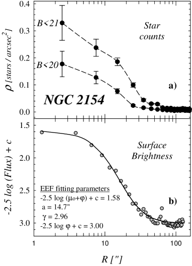
Figure 4: a) Radial density profiles for NGC 2154. Numbers indicate the limit $B$ magnitudes for each case. b) Radial flux profile for NGC 2154 (grey circles) and the EFF model fit (solid curve) together with the computed fitted parameters ($c$ is an arbitrary constant).

4.2 Observed Luminosity Function

We have constructed B-band Luminosity Functions (LFs) of the cluster region ($r<400$ pix) and of a similarly size field region (centered at $X=1500$, $Y=500$). The counts presented were corrected using the completeness factors given in Table 3 (see Sect. 3.3). The results are plotted in Fig. 5a.
In Figure 5b we present the pure cluster LF obtained by subtracting the field region LF from the cluster region LF.

Finally, we separated the data (both in the cluster region and in the field region) in two sets in order to isolate the red clump (RC) stars: those with $B<21.5$ and $B-R>1.0$, from the rest of the data (the main sequence region, MS). The resulting, field subtracted, LFs for the RC and MS regions are given in Fig. 5c and Fig. 5d, respectively.

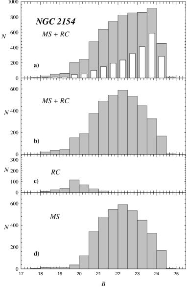
Figure 5: a) LFs corrected by completeness factors. The grey histogram corresponds to the ’cluster area’, whereas the white histogram to the ’field area’. b) LF corrected by field contamination. c) and d) Idem as panel b) but only for RC and MS regions respectively. (see Sect. 4.2).

5 Color-Magnitude Diagrams

In Fig. 6 we present the CMD of all stars measured in the complete field shown in Fig. 1. In Fig. 7 we present the CMD of the region centered at X=515, Y=1725 and having $r\leq 400$ pix (the cluster region, see Sect. 4). Although well centered in the cluster, this CMD is clearly contaminated by LMC field stars (it is interesting to note that, as it is, this CMD closely resembles that of the intermediate-age LMC cluster NGC 2173 studied by Gallart et al. (2003)).

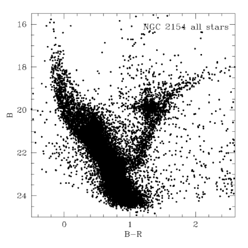
Figure 6: NGC 2154 CMD for all the measured stars.

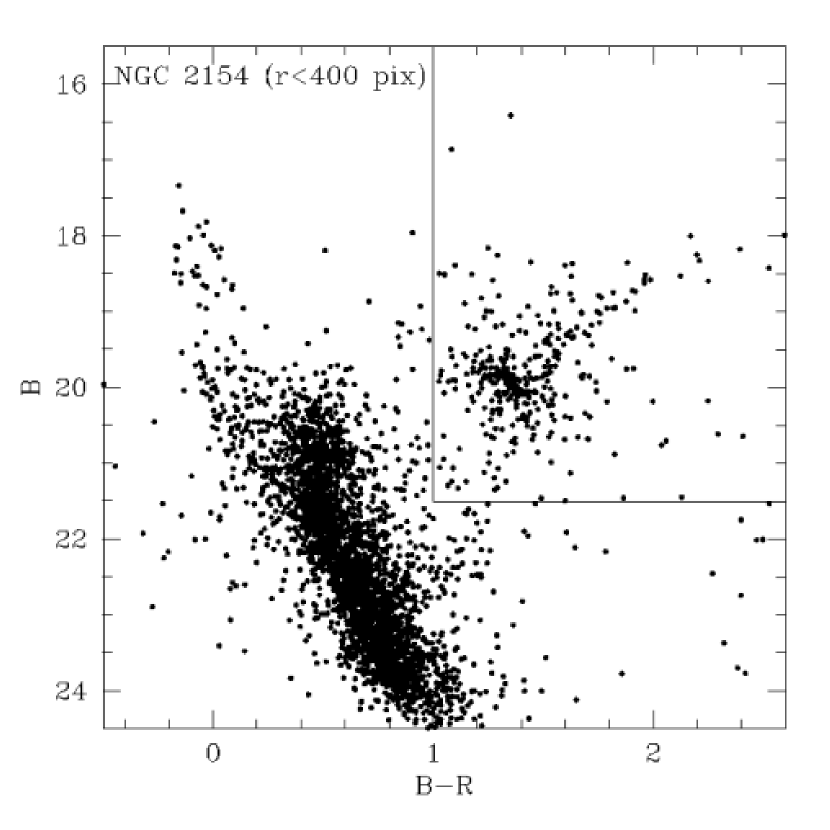
Figure 7: NGC 2154 CMD for the stars lying within 400 pixel from the cluster center. The solid line encloses the area where we looked for evolved stars.

To obtain a cleaner CMD, we applied the statistical decontamination method described in Vallenari et al. (1992) and Gallart et al. (2003). In this procedure, a statistical subtraction of field stars is carried out making a star-by-star comparison between selected reference field regions and the cluster region. Briefly, for any given star in the reference field regions we look for the most similar (in color and magnitude) star in the cluster region, and remove it from the cluster’s CMD. It should be noted that the procedure takes into account the different completeness level of the cluster and the field.

For the above purpose, we selected three reference field regions having the same area of the cluster region, which we call (see Fig. 8) Field$\#1$ (centered at X= 1500,Y=500), Field$\#2$ (centered at X=1500,Y=1500) and Field$\#3$ (centered at X=500,Y=500). They were chosen at proper distances from the cluster center, in order to avoid the presence of cluster stars in them. The results are shown in Fig. 8. The three upper panels show the CMDs of the reference fields, whereas the middle and lower panels show the corresponding CMDs of the subtracted stars, and the corresponding clean cluster CMDs, respectively.

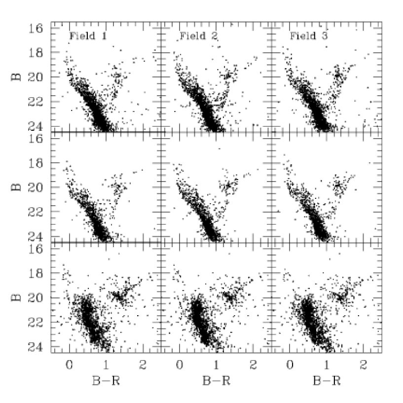
Figure 8: Field star decontamination procedure. The upper panel shows the CMDs of three different field regions. The middle panel shows the corresponding CMDs of the subtracted stars. In the lower panel the corresponding clean cluster CMDs are shown. See text for details.

Probably due to peculiarities in the distribution of field stars across the cluster region, a perfect decontamination was however not possible. Inspection of Fig. 8 shows that clean cluster regions present several groups of stars that are more numerous than in the reference field regions, despite the fact that all regions have the same area. In the clean CMDs some field stars still remain above the MS, to the left of the MS and everywhere in the red clump region. This effect surely results from the statistically low number of stars in those regions of the CMD.

Nonetheless, the procedure was very effective and helped us to improve the shape of the turnoff region (TO), and to remove several field red giant Branch (RGB) and horizontal branch stars. A careful inspection of Fig. 8 led us to adopt as the clean NGC 2154 CMD, that obtained using Field $\#3$ for the statistical decontamination (lower right panel). In this case, the subtracted field is the closest to the corresponding original field, and the number of field stars still in the cluster region is significantly lower than in the other two cases.

6 Comparison with stellar models

In this section we derive estimates of NGC 2154’s fundamental parameters by comparing its CMD with theoretical stellar evolutionary models from the Padova library of stellar tracks and isochrones (Girardi et al. 2000). These models have already been used in the past to study LMC star clusters with satisfactory results (e.g. Barmina et al. 2002, Bertelli et al. 2003). We first summarize previous work on NGC 2154 and what we know from the literature of its basic parameters.

6.1 Metallicity

Bica et al. (1986) used H$\beta$ and G-band photometry to estimate that the metallicity of NGC 2154 is $Z=0.006$. NGC 2154 was later observed by Olszewski et al. (1991) as part of a spectroscopic survey of giant stars in LMC star clusters, who derived a metallicity measuring the pseudo-equivalent width of three Ca lines. Two stars were measured with this purpose, giving an estimate of the cluster’s metallicity of [Fe/H]=-0.56$\pm$0.20. Adopting the Carraro et al. (1999) relation, this value corresponds to Z = 0.005. We shall adopt this estimate of the metallicity throughout this work.

6.2 Reddening and Distance modulus

While the distance modulus to the LMC is known with reasonable precision (Westerlund 1997, $(V_{o}-M_{V})=18.5$), no estimates of the reddening in the direction of NGC 2154 are available. To complicate matters, the reddening across the galaxy is known to be highly variable (Oestreicher & Schmidt-Kaler 1996; Zaritsky et al. 2004). As for the Galactic extinction law, here we shall use $R_{V}$=3.1 (Rieke & Lebofsky 1985).

6.3 Isochrone fitting

In Fig. 9 we have superposed three Z=0.005 ([Fe/H]= -0.60) isochrones, taken from the Girardi et al. (2000) database, to our adopted clean NGC 2154 CMD. It should be noted that this metallicity is not directly available, so it has been interpolated from different metallicity datasets. We have selected these isochrones because they provide a good fit to the MS and the TO region, and also to the magnitude and color of the RC. They have been shifted by the reddening and distance modulus indicated in the figure. The values presented for these parameters imply a corrected distance modulus of $(B_{o}-M_{B})$ in the range 18.45 to 18.50, in good agreement with the widely adopted distance modulus given by Westerlund (1997).

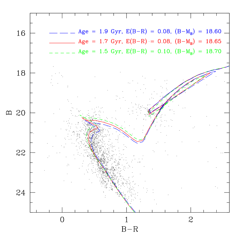
Figure 9: CMD of NGC 2154 decontaminated from field stars (see see Sect. 5). The three $Z=0.005$ isochrones superposed are from the Girardi et al. (2000) database (see Sect. 6.3).

Quick examination of Fig. 9 shows that:

• The MS is significantly wide. This may be due to a combination of observational errors, binarity, differential reddening, and age spread;

• The RGB clump is wide in color, and slightly tilted. This again can be ascribed to differential reddening and binarity;

• The stars above the TO, and outside the MS edges are mostly interlopers belonging to the LMC field in front of the cluster;

• On the other hand, the reddest field stars are probably members of the Milky Way Halo.

In the next Section we test some of these interpretations by means of synthetic CMDs.

6.4 Synthetic Color-Magnitude Diagrams and Model Luminosity Functions

Synthetic CMDs have been generated using the TRILEGAL code described in Girardi et al. (2005). The detailed procedure is outlined in Carraro et al. (2002). Using typical values derived from our observations (see Sect. 3), we have also simulated the photometric errors as a function of $B$ and $R$ magnitude.

Using our results of the isochrone fitting, we generated a synthetic CMD for a cluster which underwent an instantaneous burst of star formation 1.7 Gyr ago, and which has a population of 290 evolved stars. This number of evolved stars was derived from the luminosity function discussed in Sect. 4; and it is somewhat uncertain due to (1) possible errors while removing the contamination by the field, and (2) Poisson statistics. If we neglect for the moment the uncertainties in the field contamination, and assume the Kroupa (2001) Inital mass Function (IMF) corrected for binaries, this number of evolved stars implies a cluster mass of $33.3\pm 2.0\times 10^{3}$ $M_{\odot}$.

Our initial CMD simulation includes a fraction f=30% of detached binaries, and assumes that their mass ratio is uniformly distributed between 0.7 and 1.0. This assumption is in agreement with the observational data for the LMC clusters NGC 1818 (Elson et al. 1998), NGC 1866 (Barmina et al. 2002), and NGC 2173 (Bertelli et al. 2003). It is worth recalling that the photometry of a binary with mass ratio smaller than 0.7 is almost indistinguishable from its primary alone, so that extending the interval of simulated mass ratios would not change the results.

The results for this initial choice of parameters are shown in Fig. 10. The left panel shows the observational, decontaminated, CMD of NGC 2154 as derived in the previous section, and the right panel shows the result of our best simulation; chosen among many synthetic CMDs generated with the same input parameters but varying the random seed (Bertelli et al. 2003). The top panel presents the observational (see Sect. 4.2) ILF (Integrated Luminosity Function, solid line) together with the corresponding best fitting model ILF (dashed line).

In the simulations, special attention was given to the shape of the TO region, and to the color and magnitude of the RGB clump. Because of the complicated structure of the TO, which is broadened by the presence of binaries and the extended star formation period, for the derivation of the cluster’s distance and reddening we have used mainly the RGB clump. As can be readily seen, the mean color and magnitude of the clump has been well reproduced, allowing us to infer a reddening $E(B-R)=0.09\pm 0.02$ ($E(B-V)=0.057$), and distance modulus $(B-M_{B})_{0}=(V-M_{V})_{0}=18.48\pm 0.10$. Both these values are well within the widely accepted estimates for the LMC.

The red clump stars, however, seem to present a more elongated, tilted, distribution in the CMD, than in the initial simulation. This kind of structure might be caused by an increased fraction of binaries, by differential reddening, or by an age spread inside the cluster. All of these effects would affect not only the CMD, but also its integrated LF, and in different ways.

We have investigated these possible effects by running additional simulations in which we varied the following quantities:

• The fraction of binaries $f$, from 0 (no binaries) to 1 (each star drawn from the IMF is the primary of a system with mass ratio between 0.7 and 1) at steps of 0.1. Because the binaries are added with equal probability to both the MS and red giant part of the CMD, $f$ affects the predicted dwarf/giant ratio, and hence the ILF.

• The $1\sigma$ dispersion in reddening, between 0 and a maximum of 0.09 in $E(B-R)$. Of course, negative values of reddening are not allowed, and become 0. This causes a maximum broadening of about 0.2 mag of the red clump in $B-R$, without affecting the overall shape of the ILF.

• The duration of the star formation episode that generated the cluster, from 0 to $2.0$ Gyr, with steps of about 0.2 Gyr, centered at an age of 1.75 Gyr. This spread has a modest effect in the red clump luminosity, but affects the turn-off region of the ILF.

For each model in the grid, we compute the reduced $\chi^{2}$, defined as the mean squared difference between model and observations, in the magnitude interval $16<B<21.5$. Fainter stars are not included both because (1) below the turn-off region the ILF becomes very sensitive to the IMF, which is not known with enough accuracy; and (2) at those magnitudes the completeness corrections become large and consequently more uncertain.

The model with the lowest value of $\chi^{2}$ (=347) has $f=0.7$, $\sigma E(B-R)=0.09$ mag, and a SFH duration of 1.2 Gyr. The corresponding best fitting synthetic CMD and model ILF are presented in Fig. 11. The top panel presents the observational (see Sect. 4.2) ILF (solid line) together with the model ILF (dashed line). This theoretical ILF therefore represents the same population, with the same binary fraction, same star formation history, and photometric errors as the synthetic CMD, and with as many red giants as in the observations. It can be readily noticed that they agree reasonably well down to $B=23.5$, magnitude level at which the incompleteness corrections are still smaller than 50$\%$. It should be noticed however, that the differences between them are statistically significant, i.e. larger than the 1$\sigma$ error bars (67% confidence level) determined from the Poisson statistics.

We would like to note that a solution of similar quality, with $\chi^{2}=549$, is found for $f=0.4$, $\sigma E(B-R)=0.0$ mag, and a SFH duration of 2 Gyr. This second solution has reasonable values of $f$ (well in agreement with estimates for other LMC clusters) and $\sigma E(B-R)$. Despite the good quality of the ILF fit as measured by the $\chi^{2}$, a 2 Gyr duration for the star formation in NGC 2154 seems unacceptably long.

7 Conclusions

We have presented and discussed deep $BR$ photometry of the intermediate-age open cluster NGC 2154 in the LMC. By using theoretical tools, namely isochrones, synthetic CMDs, and an ILF, we obtained estimates of the cluster fundamental parameters. The distance and reddening found fall within the commonly accepted values for the LMC.
Very interestingly, we found that the cluster CMD, and in particular the ILF, can be properly interpreted only allowing for a extended period of star formation (1.2 Gyr). Another, less extreme, example of extended period of cluster formation, is that of the almost coeval cluster NGC 2173 in the LMC, with 0.3 Gyr (Bertelli et al. 2003). Whether the presence of such extended period of star formation is physically possible, is to be investigated in future works. From our side, it is mandatory to mention that the detection of such a prolonged star formation period could well be caused by inadequacies in the stellar evolutionary tracks themselves. The most obvious among these inadequacies is the uncertain efficiency of core convective overshooting in MS stars of masses between 1 and 2 $M_{\odot}$ (see e.g. Chiosi 2006).

An interesting point raised by the referee is whether the blue stars which concur to enlarge the MS and thicken the TO producing the extended star formation effect we find, might indeed be Blue Stragglers Stars (BSSs). These stars are ubiquitous, and they are routinely found in Dwarf Galaxies, Galactic star clusters and the general Galactic field (de Marchi et al. 2006). Unfortunately, a comprehensive search and analysis of BSSs in the LMC clusters is still unavailable.
While there is no consensus yet on the mechanism which produces these stars, their position in the CMD and their population are reasonably well understood. They occupy a strip along the extension of the MS above the TO point, but tend to be bluer than the standard binary star sequence (which runs parallel to the MS). Besides, they occupy a region of the CMD where young stars of the general stellar field toward a star cluster or a dwarf galaxy are found. This complicates their detection and demand more effective membership criteria.
In our CMD, after the cleaning procedure, most of blue stars are actually more compatible with field stars, and the shape of the TO point does not seem to be affected by classical BSSs, which instead would occupy a region which detaches from the cluster MS at B $\approx$21.5, (B-R) $\approx$0.35, following the extension of the cluster MS below the TO.
The two classical explanations for these stars are that they are binary stars or more massive stars born in a separate later star formation episode. Our simulations include both these effects in a way that it is impossible to clarify whether BSSs are present or not.
We have visually compared the CMD of NGC 2154 with the CMD of the rich star cluster NGC 2173 by Bertelli et al. (2003). The main motivation for this choice is that this study investigates a cluster -NGC 2173- which is coeval to NGC 2154 and, interestingly, the authors find that only a sizable age dispersion can explain the shape of the TO.
As in our case, the cleaned CMD of this cluster (their Figs 4 and 5) show only a few stars on the blue side of the MS, and the region right above the TO is more easily explained in terms of binary stars and extended star formation.

The fact that another coeval cluster -NGC 2173- does show the same features as NGC 2154 and can be only interpreted as having experienced long-lasting star formation might instead be telling us that the physics of TO mass stars typical of this age might have some problems, as mentioned above.

Figure 10: The observational CMD of NGC 2154 is shown in the left panel. The right panel presents a synthetic CMD of the cluster obtained for our initial choice of parameters (i.e., assuming $Z=0.005$, an age of 1.7 Gyr, and 30% of binaries). The top panel presents the observational ILF (solid line) together with best model ILF obtained with the above parameters (dashed line). 1$\sigma$ Poisson error bars are included.

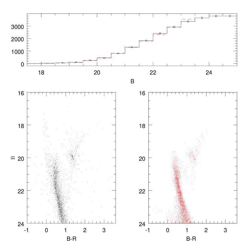
Figure 11: The observational CMD of NGC 2154 is shown in the left panel. The right panel presents our best fitting synthetic CMD of the cluster. The top panel presents the observational ILF (solid line) together with our finally adopted model ILF (dashed line). 1$\sigma$ Poisson error bars are included. See text for details.

References

- [1] Barmina R., Girardi L., Chiosi C., 2002, A&A 385, 847
- [2] Baume G., Moitinho A., Giorgi E.E., Carraro G., Vazquez R. 2004 A&A 417, 961
- [3] Bertelli G., Nasi E., Girardi L., Chiosi C., Zoccali M., Gallart C., 2003, AJ 125, 770
- [4] Bica E., Dottori H., Pastoriza M., 1986, A&A 156, 261
- [5] Carraro G., Girardi L., Chiosi C., 1999, MNRAS 309, 430
- [6] Carraro G., Girardi L., Marigo P., 2002, MNRAS 332, 705
- [7] Carraro G., Baume G., Piotto G., Méndez R.A., Schmidtobreick L., 2005, A&A 436, 527
- [8] Chiosi C., 2006, proceeding of the IAU symposium 239
- [9] de Marchi, F., de Angeli, F., Piotto, G., Carraro, G., Davies, M.B., 2006, A&A 489, 497
- [10] Elson R.A.W., Fall S.M., Freeman K.C. 1987, ApJ 323, 54
- [11] Gallart C., Zoccali M., Bertelli G., Chiosi C., Demarque P., Girardi L., Nasi E., Woo J.-H., Yi S., 2003, AJ 125, 742
- [12] Girardi L., Bressan A., Bertelli G., Chiosi C., 2000, A&AS 141, 371
- [13] Girardi L., Groenewegen M.A.T., Hatziminaoglou E., da Costa L., 2005, A&A 436, 895
- [14] Landolt A.U., 1992, AJ 104, 340
- [15] Mackey A.D., Gilmore G.F. 2003, MNRAS 338, 120
- [16] Oestreicher M., Schmidt-Kaler Th. 1996, A&AS 117, 303
- [17] Olszewski E.W., Schommer R.A., Suntzeff N.B., Harris H.C., 1991, AJ 1010, 515
- [18] Pedreros, M. Costa, E., Méndez, R.A., 2006, AJ, 131, 1461
- [19] Persson S.E., Aaronson M., Cohen J.G., Frogel J.A., Matthews K., 1983, ApJ 266, 105
- [20] Rieke G.H., Lebofsky M., 1985, ApJ 288, 618
- [21] Searle L., Wilkinson A., Bagnuolo W.G. 1980, ApJ 239, 803
- [22] Stetson P.B. 1987, PASP 99, 191
- [23] Stetson, P. B. 1992, in Stellar Photometry-Current Techniques and Future Developments, ed. C. J. Bulter, & I. Elliot (Cambridge: Cambridge University Press), IAU Coll., 136, 291
- [24] Vallenari A., Chiosi C., Bertelli G., Meylan G., Ortolani S., 1992, AJ 104, 1100
- [25] Westerlund B. 1997, in The Magellanic Clouds (Cambridge: Cambridge University Press)
- [26] Woo J.-H., Gallart C., Demarque P., Yi S., Zoccali M., 2003, AJ 125, 754
- [27] Zaritsky D., Harris J., Thompson I. B., Grebel E. K., 2004, AJ, 128, 1606