The Metallicity of Stars with Close Companions

Abstract

We examine the relationship between the frequency of close companions (stellar and planetary companions with orbital periods $<5$ years) and the metallicity of their Sun-like ($\sim$ FGK) hosts. We confirm and quantify a $\sim 4\sigma$ positive correlation between host metallicity and planetary companions. We find little or no dependence on spectral type or distance in this correlation. In contrast to the metallicity dependence of planetary companions, stellar companions tend to be more abundant around low metallicity hosts. At the $\sim 2\sigma$ level we find an anti-correlation between host metallicity and the presence of a stellar companion. Upon dividing our sample into FG and K sub-samples, we find a negligible anti-correlation in the FG sub-sample and a $\sim 3\sigma$ anti-correlation in the K sub-sample. A kinematic analysis suggests that this anti-correlation is produced by a combination of low-metallicity, high-binarity thick disk stars and higher-metallicity, lower-binarity thin disk stars.

1. Introduction

With the detection to date of more than $160$ exoplanets using the Doppler technique, the observation of Gonzalez (1997) that giant close–orbiting exoplanets have host stars with relatively high stellar metallicity compared to the average field star has gotten stronger (Reid, 2002; Santos et al., 2004; Fischer & Valenti, 2005; Bond et al., 2006). To understand the nature of this correlation between high host metallicity and the presence of Doppler-detectable exoplanets, we investigate whether this correlation extends to stellar mass companions.

There has been a widely held view that metal-poor stellar populations possess few stellar companions (Batten, 1973; Latham et al., 1988; Latham, 2004). This may have been largely due to the difficulty of finding binary stars in the galactic halo, e.g. Gunn & Griffin (1979). Duquennoy & Mayor (1991) investigated the properties of stellar companions amongst Sun-like stars but did not report a relationship between stellar companions and host metallicity. Latham et al. (2002) and Carney et al. (2005) reported a lower binarity for stars on retrograde Galactic orbits compared to stars on prograde Galactic orbits but found no dependence between binarity and metallicity within those two kinematic groups. Dall et al. (2005) speculated that the frequency of host stars with stellar companions may be correlated with metallicity in the same way that host stars with planets are.

In this paper we describe and characterize the correlation between host metallicity and the fraction of planetary and stellar companions. In Section 2 we define our sample of close planetary and stellar companions and we describe the variety of techniques used to obtain metallicities of stars that do not have spectroscopic metallicities from Doppler searches. In Section 3 we analyze the distribution of planetary and stellar companions as a function of host metallicity. We confirm and quantify the correlation between planet-hosts and high metallicity and we find a new anti-correlation between the frequency of stellar companions and high metallicity. In Section 4 we compare our stellar companion results to analogous analyses of the Nordström et al. (2004) and Carney et al. (2005) samples.

2. The Sample

We analyze the distribution of the metallicities of FGK main-sequence stars with close companions (period $<5$ years). For this we use the sample of stars analyzed by Grether & Lineweaver (2006). This subset of ‘Sun-like’ stars in the Hipparcos catalog, is defined by $0.5\leq B-V\leq 1.0$ and $5.4(B-V)+2.0\leq M_{V}\leq 5.4(B-V)-0.5$. This forms a parallelogram -0.5 and 2.0 mag, below and above an average main-sequence in the HR diagram. The stars range in spectral type from approximately F7 to K3 and in absolute magnitude in V band from 2.2 to 7.4. From this we define a more complete closer ($d<25$ pc) sample of stars and an independent more distant ($25<d<50$ pc) sample. See Grether & Lineweaver (2006) for additional details about the sample definition.

2.1. Measuring Stellar Metallicity

The metallicity of most of the extrasolar planet hosts have been determined spectroscopically. We analyse the metallicity data from three of these groups: (1) the McDonald observatory (hereafter, McD) group (e.g. Gonzalez et al., 2001; Laws et al., 2003), (2) the European Southern Observatory (hereafter, ESO) group (e.g. Santos et al., 2004, 2005), and (3) the Keck, Lick and Anglo-Australian observatory (hereafter, KLA) group (Fischer & Valenti, 2005; Valenti & Fischer, 2005).

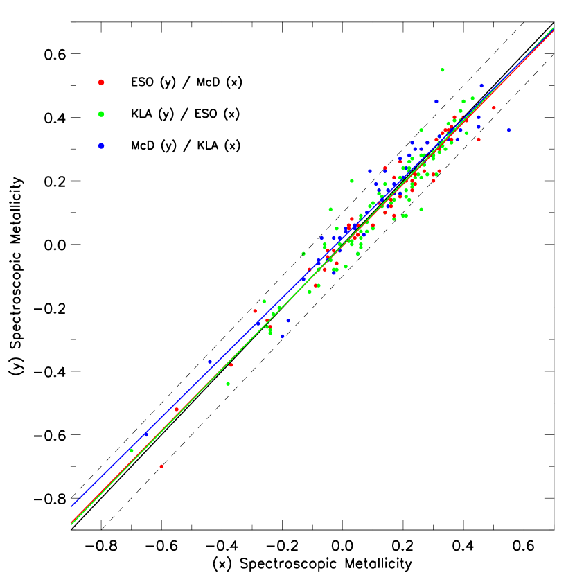
Figure 1.— Exoplanet Target Stars Metallicity Comparison. We compare the spectroscopic exoplanet target metallicities of the McD, ESO and KLA groups. The 59 red dots compare the ESO to the McD values of exoplanet target metallicity that these groups have in common. We find that the ESO values are on average $0.01$ dex smaller than the McD values with a dispersion of $0.05$ dex. Similarly the 99 green dots compare the KLA values to the average $0.01$ dex smaller ESO values with a dispersion of $0.06$ dex. The 56 blue dots compare the KLA to the average $0.01$ dex larger McD values with a dispersion of $0.06$ dex. A solid black line shows the slope-one line with dashed lines at $\pm 0.1$ dex. The three linear best-fits for these three comparisons are nearly identical to the slope-one line and almost all scatter is contained within 0.1 dex. The relationship between the McD and ESO values is very close with a marginally looser relationship to the KLA values. Thus, these values for exoplanet target metallicity are consistent at the $\sim 0.1$ dex level.

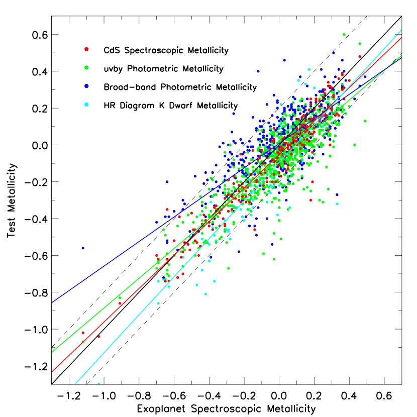
Figure 2.— Metallicity values from exoplanet spectroscopy compared to four other methods of obtaining stellar metallicities. We compare the exoplanet target spectroscopic metallicities (plotted on the $x$ axis as a ‘reference’) with the following test samples plotted on the $y$ axis: (1) CdS spectroscopic metallicities (red dots), (2) uvby photometric metallicities (green dots) (3) broad-band photometric metallicities (blue dots) and (4) HR diagram K dwarf metallicities (aqua dots). The mean differences between the test and the reference sample metallicities ($[{\rm Fe}/{\rm H}]_{\rm test}-[{\rm Fe}/{\rm H}]_{\rm ref}$) are $-0.05$, $-0.08$, $0.01$, and $-0.10$ dex respectively, with dispersions of $0.08$, $0.11$, $0.14$ and $0.14$ dex respectively. Comparing these mean differences and dispersions we find that the mean differences are within $1\sigma$ of the solid black slope-one line and thus we regard the systematic offsets as marginal. The four linear best-fits for these four comparisons (shown by the four colored lines) do not show significant deviation from the slope-one line (black) except for the metallicities derived using broad-band photometry (dark blue line).

All three of these groups find similar metallicities for the extrasolar planet target stars that they have all observed as shown by the comparisons in Fig. 1. Apart from the $\sim 1000$ KLA target stars analyzed with a consistently high precision by Valenti & Fischer (2005), many nearby ($d<50$ pc) FGK stars lack precise metallicities if they have any published measurement at all. A smaller sample of precise spectroscopic metallicities has also been published by the ESO group for non-planet hosting stars (Santos et al., 2005).

Since the large sample of KLA stars has been taken from exoplanet target lists it also has the same biases. This includes selection effects (i) against high stellar chromospheric activity (ii) towards more metal-rich stars that have a greater probability of being a planetary host and (iii) against most stars with known close ($\theta<2^{\prime\prime}$) stellar companions. We need to correct for or minimize these biases to determine quantitatively not only how the planetary distribution varies with host metallicity but also how the close stellar companion distribution varies with host metallicity, that is, we need metallicities of all stars in our sample in order to compare companion-hosting stars to non-companion-hosting stars, and to compare the metallicities of planet–hosting stars to the metallicities of stellar–companion–hosting stars.

In addition to the metallicities reported by the McD, ESO and KLA groups, we use a variety of other sources and techniques to determine stellar metallicity although with somewhat less precision. These include other sources of spectroscopic metallicities such as the Cayrel de Strobel et al. (2001) (hereafter, CdS) catalog, metallicities derived from uvby narrow-band photometry or broad-band photometry and metallicities derived from a star’s position in the HR diagram. The precision of the spectroscopic metallicity values in the CdS catalog are not well quantified. However, many of the stars in the catalog have several independent metallicity values which we average, excluding obvious outliers. To derive metallicities from uvby narrow-band photometry we apply the calibration of Martell & Smith (2004) to the Hauck & Mermilliod (1998) catalog. We also use values of metallicity derived from broad-band photometry in (Ammons et al., 2006). For stars with $5.5<M_{V}<7.3$ (K dwarfs) the relationship between stellar luminosity and metallicity is very tight (Kotoneva et al., 2002). Using this relationship, we derive metallicities for some K dwarfs from their position in the HR diagram.

Table 1Stellar Samples Used in Our Analysis

		Range	Stars with [Fe/H] Measurements
Sample	$B-V$	(pc)	Total	Binary	Targets	Planet Hosts	[Fe/H] Source
Our FGK	$0.5-1.0$	$d<25$	453	45 (9.9%)	379 (84%)	19 (5.0%)	Mostly Spec.
	$0.5-1.0$	$25<d<50$	2745	107 (3.9%)	1597 (58%)	36 (2.3%)	Mostly Phot.
Our FG	$0.5-0.75$	$d<25$	257	27 (10.5%)	228 (89%)	13 (5.7%)	Mostly Spec.
	$0.5-0.75$	$25<d<50$	1762	76 (4.3%)	1167 (66%)	32 (2.7%)	Mostly Phot.
Our K	$0.75-1.0$	$d<25$	196	18 (9.2%)	151 (77%)	6 (4.0%)	Mostly Spec.
	$0.75-1.0$	$25<d<50$	983	31 (3.2%)	430 (44%)	4 (0.9%)	Mostly Phot.
GC FGK	$0.3-1.0$	$d<40$	1375	378 (27.5%)	–	–	uvby Phot.
	$0.5-1.0$	$d<40$	1289	346 (26.8%)	–	–	uvby Phot.
GC FG	$0.5-0.75$	$d<40$	1117	291 (26.1%)	–	–	uvby Phot.
GC K	$0.75-1.0$	$d<40$	172	55 (32.0%)	–	–	uvby Phot.
CL AFGK	$0.0-1.0$	–	963	254 (26.4%)	–	–	Spec.

Note. — For notes $e$ - $j$, “HP Spec.” is high precision exoplanet target spectroscopy, “CdS Spec.” is Cayrel de Strobel et al. (2001) spectroscopy, “uvby Phot.” is uvby photometry, “BB Phot.” is broad-band photometry and “HR K Dwarf” is the method for obtaining metallicities for K dwarfs from their position in the HR diagram (Kotoneva et al., 2002).

To quantify the precision of their metallicities, we compare in Fig. 2 the different methods of determining metallicity. We use the high precision exoplanet target spectroscopic metallicities from the McD, ESO and KLA surveys (or the average when a star has two or more values) as the reference sample. We compare these metallicities with metallicities of the following test samples: (1) CdS spectroscopic metallicities, (2) uvby photometric metallicities, (3) broad-band photometric metallicities and (4) HR Diagram K dwarf metallicities.

The result of this comparison is that the uncertainties associated with the high quality exoplanet target spectroscopic metallicities of McD, ESO and KLA groups are the smallest, with the CdS spectroscopic metallicities only slightly more uncertain. The uncertainties associated with the uvby photometric metallicities are intermediate with broad-band photometric and HR diagram K dwarf metallicities being the least certain.

2.2. Selection Effects and Completeness

To minimize the scatter in the measurement of stellar metallicity while including as many stars in our samples as possible, we choose the metallicity source from one of the five groups based upon minimal dispersion. Thus we primarily use the spectroscopic exoplanet target metallicities. If no such value for metallicity is available for a star in our sample we use a spectroscopic value taken from the CdS catalog, followed by a uvby photometric value, a broad-band value and lastly a HR diagram K dwarf value for the metallicity. We use the dispersions discussed above as estimates of the uncertainties of the metallicity measurements.

Almost all $(453/464=98\%)$ of the close ($d<25$ pc) sample and $2745/2832=97\%$ of the more distant ($25<d<50$ pc) sample thus have a value for metallicity. Given the different uncertainties associated with the five sources of metallicity, the close sample has more precise values of metallicity than the more distant sample. The dispersion for the close and far sample are 0.07 and 0.10 dex respectively. See Table 1 for details.

We also investigate the color or host mass dependence of the host metallicity distributions. Thus we split our close and far samples which are defined by $0.5\leq B-V\leq 1.0$ into 2 groups, those with $0.5\leq B-V\leq 0.75$ which we call FG dwarfs and those with $0.75<B-V\leq 1.0$ which we call K dwarfs. This split is shown in Table 1. In this table we also show the total number of stars in the sample that have a known value of metallicity and the fraction that are close binaries, exoplanet target stars and exoplanet hosts.

In order to determine whether there is a real physical correlation between the presence of stellar or planetary companions and host metallicity we need to show that there are only negligible selection effects associated with the detection and measurement of these two quantities that could cause a spurious correlation. In Section 2.3 we show that the planetary companion fraction should be complete for planetary companions with periods less than 5 years for the sample of target stars that are being monitored for exoplanets. This completeness helps assure minimal spurious correlation between the probability of detecting planetary companions and host metallicity.

Table 2Metallicity and Frequency of Hosts with Close Planetary and Stellar Companions

Companions	Range	Total	Metal-poor	Sun-like	Metal-rich
Planets	$d<25$	19	2 (11%)	5 (26%)	12 (63%)
Stars	$d<25$	45	25 (56%)	14 (31%)	6 (13%)
Planets	$25<d<50$	36	3 (8%)	9 (25%)	24 (67%)
Stars	$25<d<50$	107	55 (51%)	36 (34%)	16 (15%)

The stellar companion sample is made up of two subsamples: those companions detected as part of an exoplanet survey and those that were not. The target list for exoplanets is biased against stellar binarity as discussed in Grether & Lineweaver (2006). We show that there is negligible bias between the probability of detecting stellar companions and host metallicity in two ways: (1) by showing that our close sample of stellar companions is nearly complete and (2) by using the Geneva-Copenhagen survey (hereafter, GC) of the Solar neighbourhood (Nordström et al., 2004) sample of stars, containing similar types of stars to those found in our sample, as an independent check on our results.

The GC sample of stars which contains F0-K3 stars is expected to be complete for stars with stellar companions closer than $d<40$ pc. For the close sample of stars ($d<25$ pc), the northern hemisphere of stars with close stellar companions is approximately complete. The southern hemisphere of stars is also nearly complete if we include the binary stars from Jones et al. (2002) that are likely to fall within our sample (Grether & Lineweaver, 2006). We then find that $\sim 10\%$ of stars have stellar companions with periods shorter than 5 years. If we make a small asymmetry correction (to account for the southern hemisphere not being as well monitored for binaries) we find that $\sim 11\pm 3\%$ of stars have stellar companions within this period range (Grether & Lineweaver, 2006). We also compare our sample with that of the “Carney-Latham” survey (hereafter, CL) of proper-motion stars (Carney & Latham, 1987; Carney et al., 1994) in Section 4. The CL sample also contains $\sim 11\%$ of stars with stellar companions with periods shorter than 5 years (Latham et al., 2002). We tabulate the properties of all these samples in Table 1.

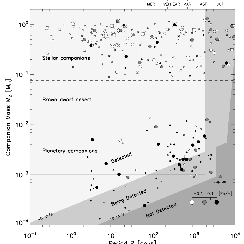
Figure 3.— Masses and periods of close companions to stellar hosts of FGK spectral type. We split the close companion sample into 3 groups defined by the metallicity of their host star: metal-poor ([Fe/H] $<-0.1$), Sun-like ($-0.1\leq$ [Fe/H] $\leq 0.1$) and metal-rich ([Fe/H] $>0.1$) which are plotted as white, grey and black dots respectively. The larger points are companions orbiting stars in the more complete $d<25$ pc sample, while the smaller points are companions to stars at distances between $25<d<50$ pc. We divide the stellar companions into those not monitored by one of the exoplanet search programs (shown with an ‘X’ behind the point) and those that are monitored. Both groups of stellar companions are distributed over the entire less-biased region (enclosed by thick line). Hence any missing stellar companions should be randomly distributed. For multiple companion systems, we select the most massive companion in our less-biased sample to represent the system.

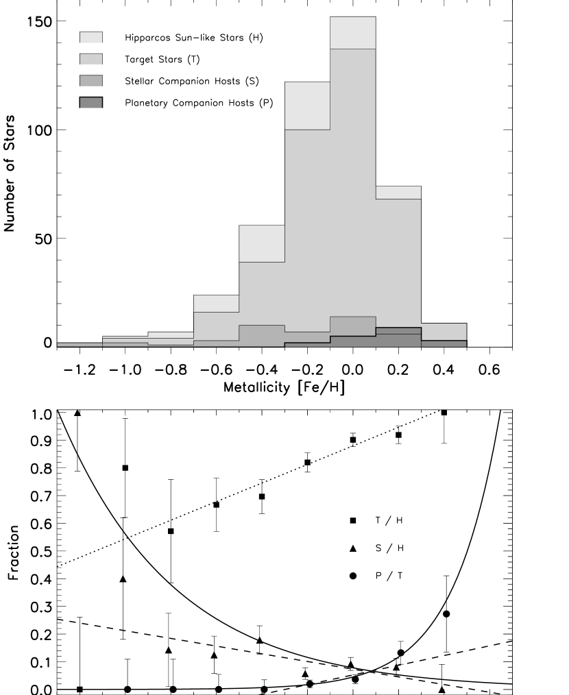
Figure 4.— Metallicities ($[{\rm Fe}/{\rm H}]$) of 453 stars in our close $d<25$ pc sample. Top: The lightest shade of grey are the Hipparcos ‘Sun-like’ stars in our close sample. The next darker shade of grey are all of the stars that are exoplanet targets. This is followed by a still darker shade of grey which are hosts of stellar companions. The darkest shade of grey are exoplanet hosts. In the Bottom plot, the fraction of target stars, stellar companion hosts and planetary companion hosts are shown by squares, triangles and circles respectively. The linear best-fit to the target fraction is shown by a dotted line. The linear and exponential best-fits to the stellar and planetary companion fractions are shown by dashed and solid lines respectively.

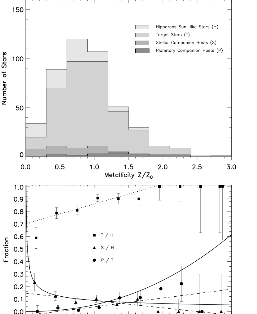
Figure 5.— Same as Fig. 4 except that metallicity is plotted linearly as ${\rm Z}/{\rm Z}_{\sun}$. All of the metal-rich (${\rm Z}/{\rm Z}_{\sun}>1.8)$ sample stars are being monitored for exoplanets but as the stellar metallicity decreases so does the fraction being monitored. This is because of a bias towards selecting more metal-rich target stars for observation due to an increased probability of planetary companions orbiting metal-rich host stars. The linear best-fit to the target fraction is shown by a dotted line. The linear and power-law best-fits to the stellar and planetary companion fractions are shown by dashed and solid lines respectively.

2.3. Close Companions

The close companions included in our $d<25$ pc and $25<d<50$ pc samples are enclosed in a rectangle of mass-period space shown in Fig. 3. These companions have primarily been detected using the Doppler technique but the stellar companions have been detected with a variety of techniques not exclusively from high precision exoplanet Doppler surveys. Thus we need to consider the selection effects of the Doppler method in order to define a less-biased sample of companions (Lineweaver & Grether, 2003). Given a fixed number of targets, the “Detected” region should contain all companions that will be found for this region of mass-period space. The “Being Detected” region should contain some but not all companions that will be found in this region and the “Not Detected” region contains no companions since the current Doppler surveys are either not sensitive enough or have not been observing for a long enough duration to detect companions in this regime. Thus as a consequence of the exoplanet surveys’ limited monitoring duration and sensitivity for our sample we only select those companions with an orbital period $P<5$ years and mass $M_{2}>0.001M_{\sun}$.

In Grether & Lineweaver (2006) we found that companions with a minimum mass in the brown dwarf mass regime were likely to be low mass stellar companions seen face on, thus producing a very dry brown dwarf desert. We also included the 14 stellar companions from Jones et al. (2002) that have no published orbital solutions but are assumed to orbit within periods of 5 years. We find one new planet and no new stars in our less biased rectangle when compared with the data used in Grether & Lineweaver (2006). This new planet HD 20782 (HIP 15527) (indicated by a vertical line through the point in Fig. 3), has been monitored for well over 5 years but only has a period of $\sim 1.6$ years and a minimum mass of $1.8M_{\rm Jup}$ placing it just between the “Detected” and “Being Detected” regions. While most planets are detected within a time frame comparable to the period, the time needed to detect this planet was much longer than its period because of its unusually high eccentricity of 0.92 (Jones et al., 2006). We thus have two groups of close companions to analyse as a function of host metallicity - giant planets and stars.

In Fig. 3 we split the close companion sample into 3 groups defined by the metallicity of their host star: metal-poor ($[{\rm Fe}/{\rm H}]<-0.1$), Sun-like ($-0.1\leq[{\rm Fe}/{\rm H}]\leq 0.1$) and metal-rich ($[{\rm Fe}/{\rm H}]>0.1$) which are plotted as white, grey and black dots respectively. Fig. 3 suggests that the hosts of planetary companions are generally metal-rich whereas the hosts of stellar companions are generally metal-poor. Table 2 and Fig. 4 confirm the correlation between exoplanets and high-metallicity and indicate an anti-correlation between stellar companions and high metallicity.

3. Close Companion - Host Metallicity Correlation

We examine the distribution of close companions as a function of stellar host metallicity in our two samples. We do this quantitatively by fitting power-law and exponential best-fits to the metallicity data expressed both linearly and logarithmically. We define the logarithmic $[{\rm Fe}/{\rm H}]$ and linear ${\rm Z}/{\rm Z}_{\sun}$ metallicity as follows:

$$[{\rm Fe}/{\rm H}]=\log({\rm Fe}/{\rm H})-\log({\rm Fe}/{\rm H})_{\sun}=\log({\rm Z}/{\rm Z}_{\sun})$$ (1)

where Fe and H are the number of iron and hydrogen atoms respectively and ${\rm Z}={\rm Fe}/{\rm H}$. We examine the close planetary companion probability $P_{\rm planet}$ and the close stellar companion probability $P_{\rm star}$ as a function of $[{\rm Fe}/{\rm H}]$ in Figs. 4 and 6 for the $d<25$ and $25<d<50$ pc samples respectively. Similarly we also examine $P_{\rm planet}$ and $P_{\rm star}$ as a function of ${\rm Z}/{\rm Z}_{\sun}$ in Fig. 5 and 7, which is effectively just a re-binning of the data in Fig. 4 and Fig. 6. We then find the linear best-fits to the planetary and stellar companion fraction distributions as shown by the dashed lines in Figs. 4-7.

We also fit an exponential to the $[{\rm Fe}/{\rm H}]$ planetary (as in Fischer & Valenti, 2005) and stellar companion fraction distributions in Figs. 4 and 6 and equivalently a power-law to the data points for the ${\rm Z}/{\rm Z}_{\sun}$ plots, Figs. 5 and 7. The two linear parameterizations that we fit to the data are:

$$P_{\rm lin\;Fe/H} = a[{\rm Fe}/{\rm H}]+P_{\sun}$$ (2)

$$P_{\rm lin\;Z/Z_{0}} = A({\rm Z}/{\rm Z}_{\sun})+(P_{\sun}-A)$$ (3)

and the two non-linear parameterizations are:

$$P_{\rm EP} = P_{\sun}10^{\alpha\;[{\rm Fe}/{\rm H}]}$$ (4)

$$= P_{\sun}({\rm Z}/{\rm Z}_{\sun})^{\alpha}$$ (5)

where $P_{\sun}$ is the fraction of stars of solar metallicity (i.e. $[{\rm Fe}/{\rm H}]=0$ and ${\rm Z}/{\rm Z}_{\sun}=1$) with companions.

If the fits for the parameters $a,A$ and $\alpha$ are consistent with zero then there is no correlation between the fraction of stars with companions and metallicity. On the other hand, a non-zero value, several sigma away from zero suggests a significant correlation ($a,A$ or $\alpha>0$) or anti-correlation ($a,A$ or $\alpha<0$).

Figure 6.— Same as Fig. 4 except for the 2745 stars in the more distant $25<d<50$ pc sample. It is harder to detect distant planets because of signal to noise considerations which limit observations to the brighter stars. This fainter, more distant sample relies more on photometric metallicity determinations than does the closer, brighter sample which has predominantly spectroscopic metallicity determinations (see Table 1). The fraction of stars being monitored for exoplanets is much lower than in Fig. 4.

Figure 7.— Same as Fig. 6 except that metallicity is plotted linearly as ${\rm Z}/{\rm Z}_{\sun}$ analogous to Fig. 5. In this more distant sample we find the same trends as in Fig. 5 but they are not as prominent.

The best-fit parameters $a,A$ and $P_{\sun}$ (but not $\alpha$) depend upon the period range and completeness of the sample. In order to compare the slopes from different samples, we parametrize this dependence in terms of the average companion fraction $P_{\rm avg}$ for the sample, i.e., if the average companion fraction for a sample is twice as large as for another sample, the best-fit slopes $a$ and $A$ as well as the fraction of stars of solar metallicity $P_{\sun}$ will also be twice as large. To compare samples with different $P_{\rm avg}$, we scale the best-fit Eqs. 2-5 to a common average companion fraction by dividing each equation by $P_{\rm avg}$. Thus, we scale the best-fit parameters $a,A$ and $P_{\sun}$ by dividing each by $P_{\rm avg}$. These scaled parameters are then referred to as $a^{\prime}=a/P_{\rm avg}$, $A^{\prime}=A/P_{\rm avg}$ and $P^{\prime}_{\sun}=P_{\sun}/P_{\rm avg}$. We list the unscaled best-fit parameters $a,A,P_{\sun},\alpha$ along with $P_{\rm avg}$ for each sample in Table 3. The parameters $a^{\prime}=a/P_{\rm avg}$ and $\alpha$ of the different samples are compared in Fig. 10.

We consistently find in Figs. 4 and 6 that metal-rich stars are being monitored more extensively for exoplanets than metal-poor stars as quantified by the “Target Stars” / “Hipparcos Sun-like Stars” ratio. This is because of a bias towards selecting more metal-rich stars for observation due to an increased probability of planetary companions orbiting metal-rich host stars. Note that this bias is well-represented by a linear trend as shown by the dotted best-fit line in these figures, and is not just a case of a few high metallicity stars being added to the highest metallicity bins. We correct for this bias by calculating “P/T” not “P/H” for each metallicity bin.

We find a correlation between $[{\rm Fe}/{\rm H}]$ and the presence of planetary companions in Fig. 4. The linear best-fit (Eq. 2) has a gradient of $a=0.18\pm 0.07$ ($\chi^{2}_{\rm red}=1.21$) and thus the correlation is significant at the $2\sigma$ level. The non-linear best-fit (Eq. 4) is $\alpha=2.09\pm 0.54$ ($\chi^{2}_{\rm red}=0.16$) and thus the correlation is significant at slightly more than the $3\sigma$ level.

Similarly we find a correlation between linear metallicity ${\rm Z}/{\rm Z}_{\sun}$ and the presence of planetary companions in the same data re-binned in Fig. 5. The linear best-fit (Eq. 3) has a gradient of $A=0.07\pm 0.03$ ($\chi^{2}_{\rm red}=1.25$) and the non-linear best-fit (Eq. 5) has an exponent of $\alpha=2.22\pm 0.39$ ($\chi^{2}_{\rm red}=1.00$) which are non-zero at the $\sim 2\sigma$ and $\sim 5\sigma$ significance levels respectively. These results are summarized in Table 3. We can compare the non-linear best-fit (Eq. 5) for linear metallicity ${\rm Z}/{\rm Z}_{\sun}$ and the non-linear best-fit (Eq. 4) for log metallicity $[{\rm Fe}/{\rm H}]$ since both contain the parameter $\alpha$. As shown by the $\chi^{2}$ per degree of freedom $\chi^{2}_{\rm red}$, the non-linear goodness of fit is better than the linear goodness of fit. We rely on the best fitting functional form which is the non-linear parameterization of our results although we use both parameterizations in our analysis.

We combine these two non-independent, non-linear best-fit estimates by computing their weighted average. We assign an error to this average by adding in quadrature (1) the difference between the two estimates and (2) the nominal error on the average. Thus our best estimate is $\alpha=2.2\pm 0.5$. Hence the correlation between the presence of planetary companions and host metallicity is significant at the $\sim 4\sigma$ level for a non-linear best-fit and at the $\sim 2\sigma$ level with a lower goodness-of-fit for a linear best-fit in our close, most complete sample.

In Fig. 4, and its re-binned equivalent Fig. 5, we find an anti-correlation between the presence of stellar companions and host metallicity. The linear stellar companion best-fits have gradients of $a=-0.14\pm 0.06$ ($\chi^{2}_{\rm red}=3.00$) and $A=-0.06\pm 0.03$ ($\chi^{2}_{\rm red}=0.91$) respectively, both significant at the $\sim 2\sigma$ level. The non-linear best-fit to the stellar companions as a function of $[Fe/H]$ in Fig. 4 is $\alpha=-0.86\pm 0.10$ ($\chi^{2}_{\rm red}=1.33$) and the non-linear best-fit to the stellar companions as a function of ${\rm Z}/{\rm Z}_{\sun}$ in Fig. 5 is $\alpha=-0.47\pm 0.18$ ($\chi^{2}_{\rm red}=0.40$). Averaging these two as above we obtain, $-0.8\pm 0.4$, which is significant at the $\sim 2\sigma$ level. All these best-fits are summarized in Table 3.

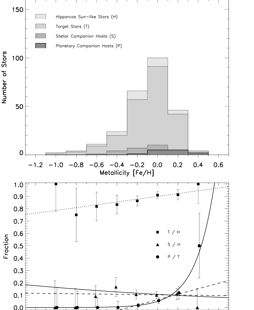
Figure 8.— Same as Fig. 4 for the stars in our close $d<25$ pc sample but only for FG dwarfs ($B-V\leq 0.75$). All stars have known metallicity in this sample. There is no apparent anti-correlation between metallicity and the presence of stellar companions.

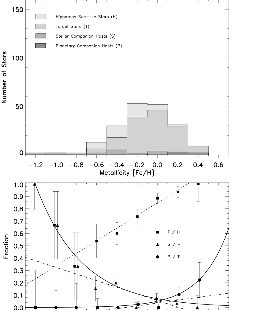
Figure 9.— Same as Fig. 4 for the stars in our close $d<25$ pc sample but only for K dwarfs ($B-V>0.75$). This plot shows a strong anti-correlation between metallicity and the presence of stellar companions.

Having found a correlation for planetary companions and an anti-correlation for stellar companions in our close sample and having found them to be robust to different metallicity binnings, we perform various other checks to confirm their reality. We check the robustness of both results to (i) distance and (ii) spectral type ($\sim$ mass) of the host star.

To check if these anti-correlations have a distance dependence, we repeat this analysis for the less complete $25<d<50$ pc sample. As shown by the best-fits in Figs. 6 and 7 and summarized in Table 3 we find only a marginal anti-correlation between the presence of stellar companions and host metallicity for the linear best-fits. The non-linear best-fits however still suggest an anti-correlation with $\alpha=-0.59\pm 0.12$ for log metallicity $[{\rm Fe}/{\rm H}]$ and $\alpha=-0.44\pm 0.12$ for linear metallicity ${\rm Z}/{\rm Z}_{\sun}$, which are significant at the $4\sigma$ and $3\sigma$ levels respectively. Combining these two estimates as described above we find $\alpha=-0.5\pm 0.2$ significant at the $2\sigma$ level in the $25<d<50$ pc sample.

The correlation between the presence of planetary companions and host metallicity for the less complete $25<d<50$ pc is significant at the $4\sigma$ and $3\sigma$ levels for the linear best-fits $a$ and $A$ respectively. The non-linear best-fit correlation has $\alpha=2.56\pm 0.45$ for log metallicity $[{\rm Fe}/{\rm H}]$ and $\alpha=3.00\pm 0.46$ for linear metallicity ${\rm Z}/{\rm Z}_{\sun}$ which are significant at the $5\sigma$ and $6\sigma$ levels respectively. Combining these two estimates we find the weighted average as above of $\alpha=2.8\pm 0.6$ significant at the $4\sigma$ level.

Having found the correlation for planetary companions and the anti-correlation for stellar companions robust to binning but less robust in the less-complete more distant sample, we test for spectral type ($\sim$ host mass) dependence. We split our sample into bluer and redder subsamples to investigate the effect of spectral type on the close-companion/host-metallicity relationship. We define the bluer subsample by $B-V\leq 0.75$ (FG spectral type stars) and the redder subsample by $B-V>0.75$ (K spectral type stars). Since $B-V$ has a metallicity dependence, a cut in $B-V$ will not be a true mass cut, but a diagonal cut in mass vs metallicity. Thus, interpreting a $B-V$ cut as a pure cut in mass introduces a spurious anti-correlation between mass and metallicity.

Table 3Best-fit Trends for Close–Companion Host–Metallicity Correlation (see Fig. 10)

	Range				Linear		Non-Linear
Sample	(pc)	Type	Figure	Companions	$a$ or $A$	$P_{\sun}$ [%]	$\alpha$	$P_{\sun}$ [%]	${P_{\rm avg}}$ [%]
	$d<25$	$[{\rm Fe}/{\rm H}]$	Fig. 4	Planets	$0.18\pm 0.07$	$4.8\pm 1.2$	$2.09\pm 0.54$	$4.5\pm 1.3$	$5.0$
	$d<25$	$[{\rm Fe}/{\rm H}]$	Fig. 4	Stars	$-0.14\pm 0.06$	$7.3\pm 1.4$	$-0.86\pm 0.10$	$7.8\pm 1.3$	$9.9$
	$d<25$	${\rm Z}/{\rm Z}_{\sun}$	Fig. 5	Planets	$0.07\pm 0.03$	$3.8\pm 2.5$	$2.22\pm 0.39$	$5.3\pm 1.4$	$5.0$
	$d<25$	${\rm Z}/{\rm Z}_{\sun}$	Fig. 5	Stars	$-0.06\pm 0.03$	$8.8\pm 3.5$	$-0.47\pm 0.18$	$8.8\pm 1.5$	$9.9$
	$d<25$	Avg.	–	Planets	–	–	$2.2\pm 0.5$	–	–
Our	$d<25$	Avg.	–	Stars	–	–	$-0.8\pm 0.4$	–	–
FGK	$25<d<50$	$[Fe/H]$	Fig. 6	Planets	$0.04\pm 0.01$	$1.6\pm 0.4$	$2.56\pm 0.45$	$2.3\pm 0.5$	$2.3$
	$25<d<50$	$[Fe/H]$	Fig. 6	Stars	$-0.00\pm 0.02$	$3.3\pm 0.4$	$-0.59\pm 0.12$	$3.5\pm 0.4$	$3.9$
	$25<d<50$	$Z/Z_{\sun}$	Fig. 7	Planets	$0.03\pm 0.01$	$2.0\pm 0.6$	$3.00\pm 0.46$	$2.0\pm 0.4$	$2.3$
	$25<d<50$	$Z/Z_{\sun}$	Fig. 7	Stars	$-0.01\pm 0.01$	$3.4\pm 0.8$	$-0.44\pm 0.12$	$3.6\pm 0.4$	$3.9$
	$25<d<50$	Avg.	–	Planets	–	–	$2.8\pm 0.6$	–	–
	$25<d<50$	Avg.	–	Stars	–	–	$-0.5\pm 0.2$	–	–
	$d<25$	$[Fe/H]$	Fig. 8	Planets	$0.22\pm 0.09$	$6.3\pm 1.7$	$2.33\pm 0.62$	$5.0\pm 1.7$	$5.7$
Our	$d<25$	$[Fe/H]$	Fig. 8	Stars	$-0.01\pm 0.08$	$10.3\pm 2.0$	$-0.18\pm 0.37$	$10.7\pm 2.1$	$10.5$
FG	$25<d<50$	$[Fe/H]$	–	Planets	$0.05\pm 0.02$	$2.0\pm 0.5$	$2.63\pm 0.46$	$2.8\pm 0.6$	$2.7$
	$25<d<50$	$[Fe/H]$	–	Stars	$0.04\pm 0.02$	$4.4\pm 0.6$	$-0.09\pm 0.18$	$4.7\pm 0.6$	$4.3$
	$d<25$	$[Fe/H]$	Fig. 9	Planets	$0.11\pm 0.10$	$3.6\pm 2.0$	$1.57\pm 0.85$	$5.1\pm 3.1$	$4.0$
Our	$d<25$	$[Fe/H]$	Fig. 9	Stars	$-0.27\pm 0.07$	$5.7\pm 1.9$	$-0.95\pm 0.14$	$7.1\pm 2.3$	$9.2$
K	$25<d<50$	$[Fe/H]$	–	Planets	$0.03\pm 0.03$	$0.9\pm 0.6$	$2.10\pm 2.16$	$1.3\pm 1.0$	$0.9$
	$25<d<50$	$[Fe/H]$	–	Stars	$-0.06\pm 0.02$	$2.0\pm 0.5$	$-1.12\pm 0.19$	$2.0\pm 0.5$	$3.2$
GC FGK	$d<40$	$[Fe/H]$	Fig. 12	Stars	$-0.15\pm 0.05$	$24.0\pm 1.5$	$-0.28\pm 0.07$	$23.9\pm 1.4$	$26.8$
GC FG	$d<40$	$[Fe/H]$	Fig. 13	Stars	$-0.05\pm 0.06$	$25.1\pm 1.6$	$-0.08\pm 0.10$	$25.5\pm 1.6$	$26.1$
GC K	$d<40$	$[Fe/H]$	Fig. 14	Stars	$-0.46\pm 0.10$	$22.3\pm 3.6$	$-0.52\pm 0.11$	$23.7\pm 3.9$	$32.0$
CL AFGK	–	$[Fe/H]$	–	Stars	$-0.07\pm 0.06$	$21.3\pm 3.4$	$-0.12\pm 0.09$	$21.6\pm 3.1$	$25.7$
Combined	–	$[Fe/H]$	Fig. 15	Stars	$-0.10\pm 0.03$	$20.5\pm 1.3$	$-0.22\pm 0.05$	$20.7\pm 1.2$	$25.7$

The linear best-fit to the stellar companions of the FG sample ($d<25$ pc) has a normalised gradient of $a^{\prime}=(-0.01\pm 0.08)/10.5\%=-0.1\pm 0.8$ and the non-linear best-fit is $\alpha=-0.2\pm 0.4$ as shown in Fig. 8. Both of these best-fits are consistent with the frequency of stellar companions being independent of host metallicity. The linear best-fit to the stellar companions of the K sample has a gradient of $a^{\prime}=(-0.27\pm 0.07)/9.2\%=2.9\pm 0.8$ and the non-linear best-fit is $\alpha=-1.0\pm 0.1$ as shown in Fig. 9 for the close $d<25$ pc stars. Both of these best-fits show an anti-correlation between the presence of stellar companions and host metallicity at above the $3\sigma$ level. Less significant results are obtained for the $25<d<50$ FG and K spectral type samples with stellar companions as shown in Table 3.

These results suggest that the observed anti-correlation between close binarity and host metallicity is either (i) real and stronger for K spectral type stars than for FG stars or (ii) due to a spectral-type dependent selection effect.

Under the hypothesis that the anti-correlation between host metallicity and binarity is real for K dwarfs, there is a possible selection effect limited to F and G stars that could explain why we do not see the anti-correlation as strongly in them. Doppler broadening of the line profile, due to random thermal motion in the stellar atmosphere and stellar rotation, both increase in more massive F and G stars due to their higher effective temperature and faster rotation speeds compared with less massive K stars. This wider line profile for F and G stars results in fewer observable shifting lines thus lowering the spectroscopic binary detection efficiency. However we directly examine the stellar companion fraction as a function of spectral type or color $B-V$ in Fig. 11. For both single-lined and double-lined spectroscopic binaries, if the binary detection efficiency was systemically higher for K dwarfs then the anti-correlation could be a selection effect. However we find that it is fairly independent of spectral type. Thus the anti-correlation does not appear to be a spectral-type dependent selection effect.

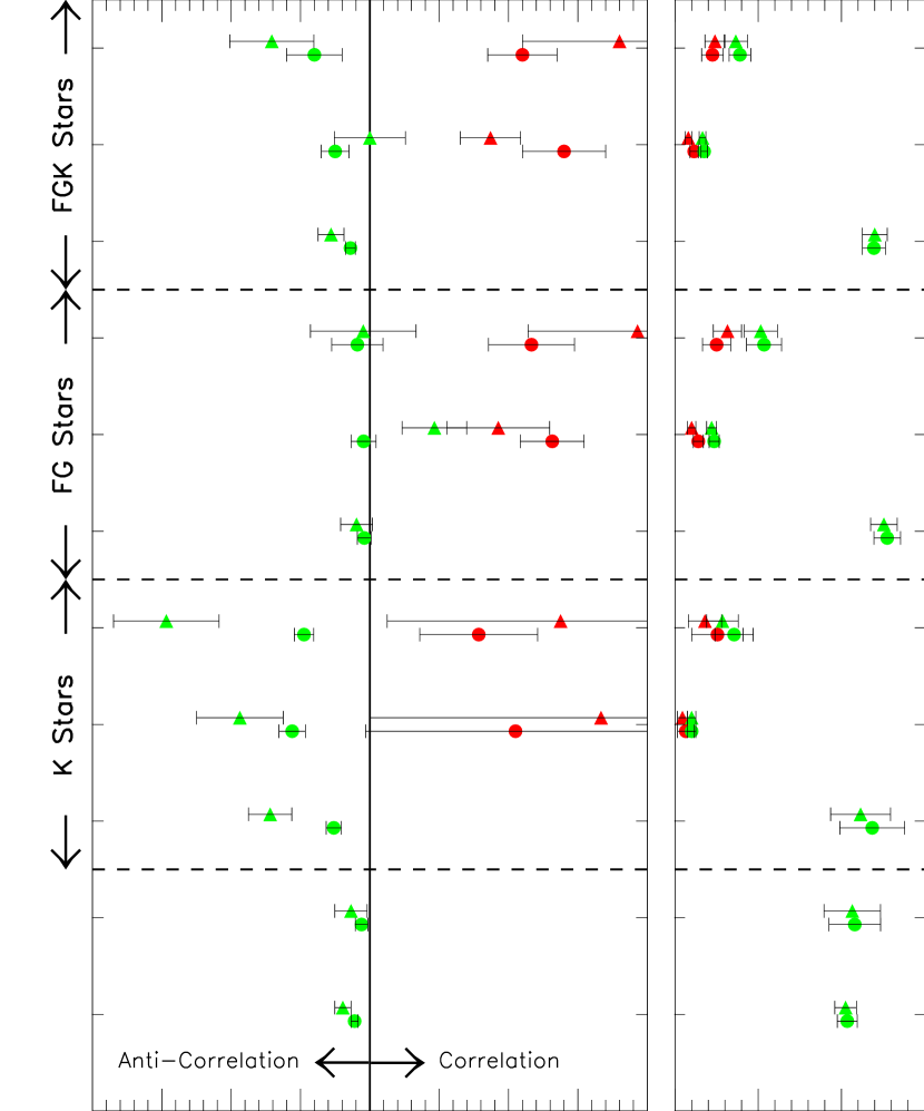
Figure 10.— We compare the linear $a^{\prime}$ (triangles) and non-linear $\alpha$ (circles) parameterizations for the various samples listed in Table 3. The red points are the best-fits to planetary companions and the green points the best-fits to stellar companions. The fact that the red planet values for $\alpha$ are significantly larger than zero confirms and quantifies the metallicity/planet correlation. The fact that the green stellar values for $\alpha$ are predominantly less than zero, significantly so only for K dwarfs, is a surprising new result. The labels on the RHS refer to the samples for which the best-fit parameterizations are valid. We normalize the linear parametrization by dividing the best-fit gradient $a$ by the average companion fraction $P_{\rm avg}$ (see text). This plot is a graphical version of Table 3 whose notes also apply to this plot. All of the best-fits are from $[{\rm Fe}/{\rm H}]$ plots except for our FGK stars where $\alpha$ is the average of the best-fits to both the $[{\rm Fe}/{\rm H}]$ and ${\rm Z}/{\rm Z}_{\sun}$ plots. The $P_{\sun}$ values plotted in the vertical panel on the right refer to the corresponding best-fit normalization at solar metallicity (Eqs. 2-5).

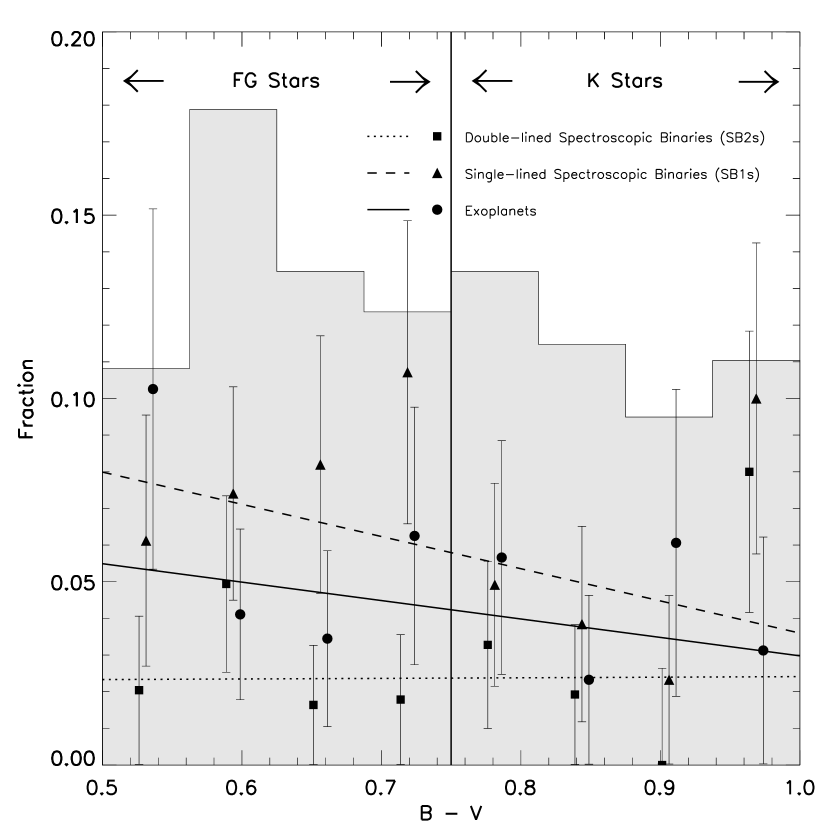
Figure 11.— Color ($B-V$) distribution for double-lined (squares) and single-lined (triangles) spectroscopic binaries (SB2s and SB1s respectively) and exoplanets (circles) in our close $d<25$ pc sample. The linear best-fit gradient for SB2s is $0.00\pm 0.06$, for SB1s it is $-0.08\pm 0.08$ and for exoplanets it is $-0.05\pm 0.08$. All three of these gradients are only significant at $\mbox{$\>\stackrel{{\scriptstyle<}}{{{}_{\sim}}}\>$}1\sigma$ level. There is no significant correlation between SB1, SB2 or planetary fraction for either FG ($B-V\leq 0.75$) stars or for K ($B-V>0.75$) stars.

We also examine the spectral type ($\sim$ mass) dependence of the correlation between planetary companions and host metallicity. The linear best-fit to the planetary companions of the FG sample has a gradient of $a^{\prime}=(0.22\pm 0.09)/5.7\%=3.9\pm 1.6$ and the non-linear best-fit is $\alpha=2.3\pm 0.6$ as shown in Fig. 8 for the close $d<25$ pc stars. These are significant at the 2 and 3 $\sigma$ levels respectively. The linear best-fit to the planetary companions of the K sample has a gradient of $a^{\prime}=(0.11\pm 0.10)/4.0\%=2.8\pm 2.5$ and the non-linear best-fit is $\alpha=1.6\pm 0.9$ as shown in Fig. 9 for the close $d<25$ pc stars. These are both significant at between the 1 and 2 $\sigma$ levels. The K sample contains fewer planetary and stellar companions compared to the FG sample. Both the linear and non-linear fits are consistent between the FG and K samples suggesting that the correlation between the presence of planetary companions and host metallicity is independent of spectral type and consequently host mass. The fraction of planetary companions is also fairly independent of spectral type as shown in Fig. 11.

Thus our results suggest that the correlation between the presence of planetary companions and host metallicity is significant at the $\sim 4\sigma$ level and that the anti-correlation between the presence of stellar companions and host metallicity is significant at the $\sim 2\sigma$ for the $d<25$ pc FGK sample. Splitting both samples into FG and K spectral type stars suggests that the correlation between the presence of planetary companions and host metallicity is independent of spectral type but that the anti-correlation between the presence of stellar companions and host metallicity is a strong function of spectral type with the anti-correlation disappearing for the bluer FG host stars (see Fig. 10). We find no spectral-type dependent binary detection efficiency bias that can explain this anti-correlation.

4. Is the Anti-Correlation between Metallicity and Stellar Binarity Real?

We further examine the relationship between stellar metallicity and binarity by comparing our sample with that of the Geneva and Copenhagen survey (GC) of the solar neighbourhood (Nordström et al., 2004) that has been selected as a magnitude-limited sample, a volume-limited portion ($d<40$ pc) of which we analyse. This selection criteria infers that the sample is kinematically unbiased, i.e., the sample contains the same proportion of thin, thick and halo stars as is found in the solar neighbourhood. We also compare our sample with that of the “Carney-Latham” survey (CL) that has been kinematically selected to have high proper motion stars (Carney & Latham, 1987), i.e., it contains a larger proportion of halo stars compared to disk stars than is observed for the solar neighbourhood.

Our sample is based on the Hipparcos sample that has a limiting magnitude for completeness of $V=7.9+1.1\sin|b|$ (Reid, 2002) where $b$ is Galactic latitude. Thus the Hipparcos sample is more complete for stars at higher Galactic latitudes where the proportion of halo stars to disk stars increases. Hence our more distant ($25<d<50$ pc) sample will have a small kinematic bias in that it will have an excess of halo stars, whereas our closer ($d<25$ pc) sample will be less kinematically biased.

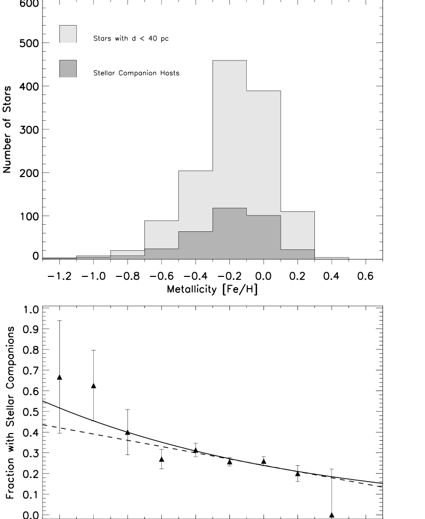
Figure 12.— Histogram of stars in the complete volume limited GC sample ($d<40$ pc). We exclude those stars with $b-y<0.3$ so that the spectral type range becomes F7-K3 and thus similar to that of our sample. We only include those stars that have between 2 and 10 radial velocity measurements with the CORAVEL spectrograph. We find an anti-correlation between binarity and host metallicity as shown by the linear and non-linear best-fits represented by the dashed and solid lines respectively.

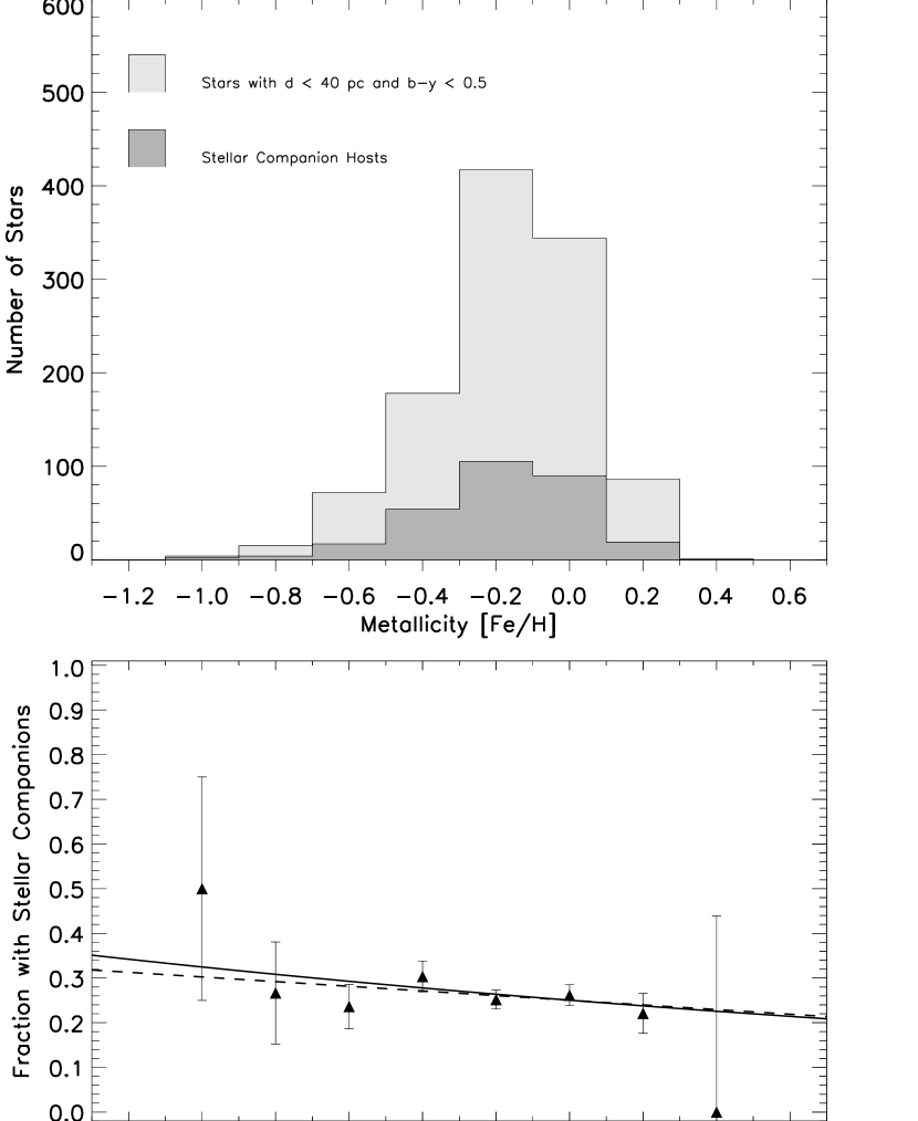
Figure 13.— Same as Fig. 12 but only for the FG dwarfs in the GC sample of stars ($d<40$ pc). We define FG dwarfs as those with $b-y<0.5$ ($B-V\mbox{$\>\stackrel{{\scriptstyle<}}{{{}_{\sim}}}\>$}0.75$). We find only a marginal anti-correlation between binarity and host metallicity as shown by the linear best-fit with gradient $a=-0.05\pm 0.06$ and the non-linear best-fit with $\alpha=-0.11\pm 0.10$. Using $P_{\rm avg}=26.1\%$, the scaled linear gradient $a^{\prime}=(-0.05\pm 0.06)/26.1\%=-0.2\pm 0.2$.

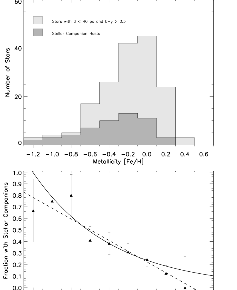
Figure 14.— Same as Fig. 12 but only for the K dwarfs in the GC sample of stars ($d<40$ pc). We define K dwarfs as those with $b-y>0.5$ ($B-V\mbox{$\>\stackrel{{\scriptstyle>}}{{{}_{\sim}}}\>$}0.75$). We find a very strong anti-correlation between binarity and host metallicity as shown by the linear best-fit with gradient $a=-0.46\pm 0.10$. The non-linear best-fit is $\alpha=-0.52\pm 0.11$. The scaled linear gradient $a^{\prime}=(-0.46\pm 0.10)/32.0\%=-1.4\pm 0.3$. Comparing this plot with Fig. 13 suggests that the anti-correlation between binarity and host metallicity is stronger for redder stars.

4.1. Comparison with a Kinematically Unbiased Sample

The GC sample contains primarily F and G dwarfs with apparent visual magnitudes $V\mbox{$\>\stackrel{{\scriptstyle<}}{{{}_{\sim}}}\>$}9$ and is complete in volume for $d<40$ pc for F0-K3 spectral type stars. Unlike our sample analyzed in Section 3, it also includes early F spectral type stars. The GC sample color range is defined in terms of $b-y$ not $B-V$ like our samples. We remove these early F stars with $b-y<0.3$ ($B-V\mbox{$\>\stackrel{{\scriptstyle<}}{{{}_{\sim}}}\>$}0.5$, Cox, 2000) from the sample so that the GC sample spectral type range is similar to ours. The GC sample then ranges from $0.3\leq b-y\leq 0.6$ ($0.5\mbox{$\>\stackrel{{\scriptstyle<}}{{{}_{\sim}}}\>$}B-V\mbox{$\>\stackrel{{\scriptstyle<}}{{{}_{\sim}}}\>$}1.0$) with those stars above $b-y=0.5$ ($B-V\sim 0.75$) referred to as K stars. We also exclude suspected giants from the GC sample.

For the GC sample, we only include those binaries observed by CORAVEL between 2 and 10 times so as to avoid a potential bias where low metallicity stars were observed more often, thus leading to a higher efficiency for finding binaries around these stars. This homogenizes the binary detection efficiency such that any real signal will not be removed by such a procedure. Unlike our sample for which we only include binaries with $P<5$ years, the GC sample also includes much longer period visual binaries in addition to short period spectroscopic binaries such that the total binary fraction of all types corresponds to $\sim 25\%$. Comparing this with the period distribution for G dwarf stars of Duquennoy & Mayor (1991) this binary fraction corresponds to binary systems with periods less than $\sim 10^{5}$ days.

For the volume limited $d<40$ pc sample we again find an anti-correlation between binarity and stellar host metallicity as shown in Fig. 12. Both the linear and non-linear best-fits listed in Table 3 are significant at or above the $3\sigma$ level. We also split the GC sample into FG and K spectral type stars in Figs. 13 and 14 respectively. The anti-correlation between the presence of stellar companions and host metallicity is significant at less than the $1\sigma$ level for FG stars but significant at the $\sim 4\sigma$ level for K stars.

These results are qualitatively the same as those found for our sample but quantitatively weaker as shown in Fig. 10 (confer rows of points labeled GC). This may be due to the higher fraction of late F and early G spectral type stars compared to our samples or the larger range ($\sim 10^{5}$ days) in binary periods contained in the GC sample compared to our sample where $P<5$ years. Another way of interpreting this anti-correlation between binarity and metallicity may be in terms of the age and nature of different components of the Galaxy described by stellar kinematics, i.e., F stars are generally younger than K stars and thus are more likely to belong to the younger thin disk star population than the older thick disk star population. Hence we examine our results in terms of stellar kinematics.

4.2. Comparison with a Kinematically Biased Sample

We also compare our samples and that of the GC survey with the Carney & Latham (1987) high proper motion survey (CL). The CL survey contains all of the A, F and early G, many of the late G and some of the early K dwarfs from the Lowell Proper Motion Catalog (Giclas et al., 1971, 1978) and which were also contained in the NLTT Catalog (Luyten, 1979, 1980). The number of stars in this distribution increases as the stellar colors become redder, peaking at about $B-V=0.65$, following which the numbers of stars begin to decrease (Carney et al., 1994). This group has also obtained data for a smaller number of stars from the sample of Ryan (1989) who sampled sub-dwarfs (metal-poor stars beneath the main-sequence) that have a high fraction of halo stars in the range $0.35<B-V<1.0$. We refer to this combined sample as outlined in Carney et al. (2005) as the CL sample. This CL sample contains all binaries detected as spectroscopic binaries, visual binaries or common proper motion pairs.

In Fig. 15 we plot the binary fraction of stars on prograde and retrograde Galactic orbits as shown in Fig. 3 of Carney et al. (2005). All of the CL stars have $[{\rm Fe}/{\rm H}]\leq 0.0$. The CL distribution contains a small subset of metal-poor $[{\rm Fe}/{\rm H}]\leq-0.2$ stars from Ryan (1989) that has a one-third lower prograde binary fraction due to fewer observations. Thus stars with metallicities of between $-0.2$ and $0.0$ have a higher binary fraction than the rest of the CL distribution. We make a small correction for this bias in the binary fraction in the range $-0.2<[{\rm Fe}/{\rm H}]<0.0$ by lowering the 2 highest metallicity prograde points of the CL distribution by $2\%$.

We note an anti-correlation between the binary fraction and metallicity for $-1.3<[{\rm Fe}/{\rm H}]<0.0$ range of prograde disk stars of the CL distribution as shown in Fig. 15. We find that the linear best-fit to this anti-correlation has a gradient of $a=-0.07\pm 0.06$ and the non-linear best-fit has $\alpha=-0.12\pm 0.09$, which are both significant at slightly above the $1\sigma$ level. For consistency we exclude the two lowest metallicity points from this best-fit so that we analyse the same region of metallicity as our samples and the GC sample and because these two low metallicity points will probably contain a significant fraction of halo stars. The average binary fraction is $P_{\rm avg}=26\%$ for the disk-dominated part of the prograde CL distribution. Carney et al. (2005) found no correlation between binarity and host metallicity for the retrograde halo stars.

We overplot our $d<25$ pc binary fraction (from Fig. 4) along with the GC $d<40$ pc binary fraction (from Fig. 12) onto the prograde CL sample in Fig. 15. All three of these samples have different binary period ranges and levels of completeness. We scale our sample and the GC sample to the size of the Carney et al. (2005) sample by scaling the distributions to contain the same number of binary stars at solar metallicity. The most metal-poor point in our close binary distribution is scaled above $100\%$, hence we set this point to $100\%$. The combined three sample distribution shows an anti-correlation between binarity and metallicity. The normalized linear best-fit to this is $a^{\prime}=(-0.10\pm 0.03)/25.7\%=-0.39\pm 0.12$ and the non-linear best-fit is $\alpha=-0.22\pm 0.05$ which are both significant at or above the $\sim 3\sigma$ level (see last row of Table 3). This combined result is our best estimate and indicates a strong anti-correlation between stellar companions and metallicity for $[{\rm Fe}/{\rm H}]>-1.3$.

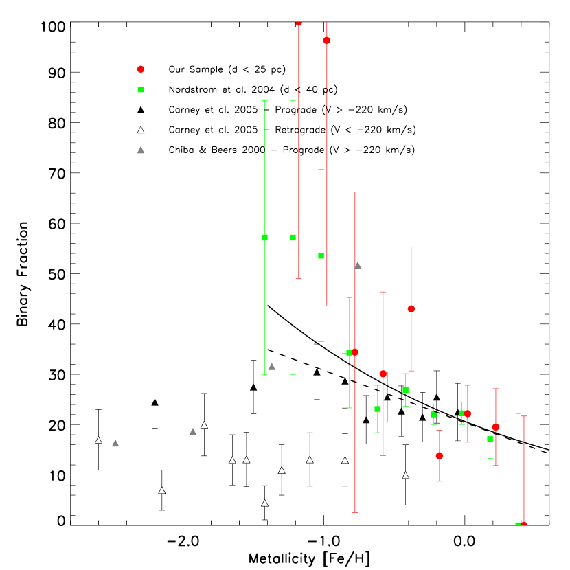
Figure 15.— This plot is adapted from Fig. 3 of Carney et al. (2005). The black triangles are the points from the CL sample of proper motion stars with prograde Galactic tangential velocities. We overplot the binary fraction as a function of host metallicity for our close ($d<25$ pc) F7-K3 sample (Fig. 4) with red circles and the green squares are from the volume limited GC sample ($d<40$ pc) for F7-K3 stars (Fig. 12). The three samples contain different average binary fractions because the period range and the levels of completeness of the stellar companions varies between the samples as discussed in the text. We normalise the distributions by scaling our sample and the GC sample so that they contain the same fraction of binary stars as the sample of Carney et al. (2005) at $[{\rm Fe}/{\rm H}]=0$. The linear and non-linear best-fits to the three samples combined are shown as dashed and solid lines respectively.

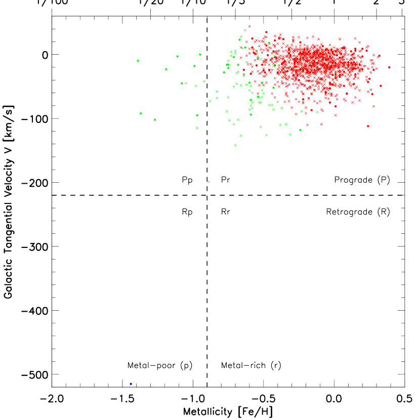
Figure 16.— We plot tangential Galactic velocity $V$ as a function of metallicity $[{\rm Fe}/{\rm H}]$ for the kinematically unbiased GC sample ($d<40$ pc). We use a probabilistic method to assign the stars in the GC sample to the three Galactic populations (halo, thick and thin disks) as discussed in the Appendix. Red points are thin disk stars, green points are thick disk stars and a blue point is the single halo star in the sample at $V<-500$ km/s. Crosses represent FG spectral-type stars and circles K stars. The ratio of thick/thin disk stars is $\sim 3$ times higher for K stars than for FG stars.

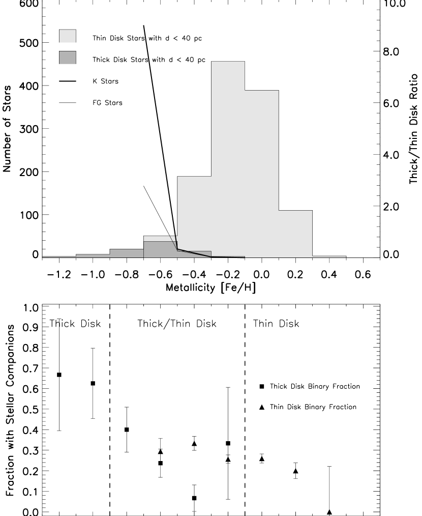
Figure 17.— Histogram of the stars in Fig. 16 suspected of belonging to the thick disk and the thin disk in the GC sample ($d<40$ pc). Notice the difference by a factor $\sim 2$ between the higher binary fraction thick disk stars and the lower binary fraction thin disk stars. We note that the K star distribution contains a higher ratio of thick disk stars than the FG star distribution in the thick/thin disk overlap region.

4.3. Discussion

We examine our results in terms of Galactic populations by determining the most likely population membership (halo, thick or thin disk) for each star in the GC sample using the method outlined in the Appendix and then plotting them in the Galactic tangential velocity $V$ - metallicity $[{\rm Fe}/{\rm H}]$ plane as in Fig. 16. We use red points for the thin disk stars, green points for the thick disk stars and a blue point for the single halo star. The kinematically unbiased GC sample contains mostly thin disk stars. Excluding the one halo star in the GC sample, stars with $[{\rm Fe}/{\rm H}]\mbox{$\>\stackrel{{\scriptstyle<}}{{{}_{\sim}}}\>$}-0.9$ belong to the thick disk and stars with $[{\rm Fe}/{\rm H}]\mbox{$\>\stackrel{{\scriptstyle>}}{{{}_{\sim}}}\>$}-0.1$ belong to the thin disk. The region $-0.9\mbox{$\>\stackrel{{\scriptstyle>}}{{{}_{\sim}}}\>$}[{\rm Fe}/{\rm H}]\mbox{$\>\stackrel{{\scriptstyle>}}{{{}_{\sim}}}\>$}-0.1$ contains a combination of both thick and thin disk stars.

We also plot these thick and thin disk stars as separate histograms in metallicity in Fig. 17. In the region $[{\rm Fe}/{\rm H}]\mbox{$\>\stackrel{{\scriptstyle<}}{{{}_{\sim}}}\>$}-0.9$ that contains only thick disk stars, we find that the binary fraction is approximately twice as large as for the region $[{\rm Fe}/{\rm H}]\mbox{$\>\stackrel{{\scriptstyle>}}{{{}_{\sim}}}\>$}-0.1$ that contains only thin disk stars. In both of these single population regions the binary fraction also appears to be approximately independent of metallicity. While our purely probabilistic method of assigning the stars in the GC sample to Galactic populations is useful for determining the general regions of parameter space that the individual populations occupy, it is not precise enough to show exactly which stars belong to which population. This is especially true for the regions of parameter space that have large overlaps such as that between the thick and thin disk stars in Fig. 16. Thus the thin and thick disk binary fractions in the interval $-0.9\mbox{$\>\stackrel{{\scriptstyle<}}{{{}_{\sim}}}\>$}[{\rm Fe}/{\rm H}]\mbox{$\>\stackrel{{\scriptstyle<}}{{{}_{\sim}}}\>$}-0.1$ are probably mixtures. We suspect that the thin and thick disk binary fractions in this overlap region will remain at the same levels as found for the non-overlapping regions. The anti-correlation between binarity and metallicity in the $-0.9\mbox{$\>\stackrel{{\scriptstyle<}}{{{}_{\sim}}}\>$}[{\rm Fe}/{\rm H}]\mbox{$\>\stackrel{{\scriptstyle<}}{{{}_{\sim}}}\>$}-0.1$ range may be due to this overlap between higher binarity thick disk stars and lower binarity thin disk stars.

We now partition the Galactic tangential velocity $V$ - metallicity $[{\rm Fe}/{\rm H}]$ parameter space into four quadrants. We split the $V$ parameter space into those stars on prograde Galactic orbits (P) and those on retrograde Galactic orbits (R). We split the $[{\rm Fe}/{\rm H}]$ parameter space into those stars that are metal rich (r) with $[{\rm Fe}/{\rm H}]\mbox{$\>\stackrel{{\scriptstyle>}}{{{}_{\sim}}}\>$}-0.9$ and those that are metal poor (p) with $[{\rm Fe}/{\rm H}]\mbox{$\>\stackrel{{\scriptstyle<}}{{{}_{\sim}}}\>$}-0.9$. We then label these quadrants by the direction of Galactic orbital motion followed by the range in metallicity or Pp, Pr, Rr and Rp as shown in Fig. 16. We now assume that the Pp quadrant contains a mixture of halo and thick disk stars and that the Pr quadrant contains a mixture of thin and thick disk stars and that the Rp and Rr quadrants only contain halo stars.

The combined anti-correlation between binarity and metallicity in Fig. 15, that all three samples appear to have in common, is predominantly in the Pr quadrant of $V-[{\rm Fe}/{\rm H}]$ parameter space that contains a mixture of thick and thin disk stars. As discussed above this anti-correlation may be due to the overlap of high binarity thick disk stars and lower binarity thin disk stars.

While Latham et al. (2002) suggest that the halo and disk populations have the same binary fraction, Carney et al. (2005) find lower binarity in retrograde stars. As shown in Fig. 15 there is a clear difference of about a factor of 2 in the region $[{\rm Fe}/{\rm H}]\mbox{$\>\stackrel{{\scriptstyle>}}{{{}_{\sim}}}\>$}-0.9$ between the binary fractions of prograde disk stars compared to retrograde halo stars (Pr and Rr respectively). All the retrograde halo stars appear to have the same binary fraction (quadrants Rr and Rp). The Pp quadrant contains prograde halo stars and has a $\sim 2$ times higher binary fraction than the quadrants containing retrograde halo stars. However the Pp quadrant also contains thick disk stars in addition to prograde halo stars.

We propose that the Pp region, $[{\rm Fe}/{\rm H}]\mbox{$\>\stackrel{{\scriptstyle<}}{{{}_{\sim}}}\>$}-0.9$, for stars on prograde Galactic orbits contains a mixture of low binarity halo stars and high binarity thick disk stars. In Fig. 15 at $[{\rm Fe}/{\rm H}]\sim-0.9$ our close sample ($d<25$ pc) and the GC sample ($d<40$ pc) start to diverge from the data points of the CL survey. This observed divergence may be due to the CL survey being comprised of high proper motion stars and consequently a higher fraction of prograde halo stars compared to thick disk stars than the kinematically unbiased GC sample and our relatively kinematically unbiased sample where thick disk stars probably numerically dominate over halo stars.

Using a kinemically unbiased sample, Chiba & Beers (2000) report that for the three regions $-1.0>[{\rm Fe}/{\rm H}]>-1.7$, $-1.7>[{\rm Fe}/{\rm H}]>-2.2$ and $-2.2>[{\rm Fe}/{\rm H}]$ that the fraction of stars that belong to the thick disk are $29\%$, $8\%$ and $5\%$ respectively, with the rest belonging to the halo. We restrict these thick disk fraction estimates to stars only on prograde orbits by assuming that all of the thick disk stars are on prograde orbits and that half of the halo stars are prograde and the other half are retrograde. Thus the fraction of prograde stars that are thick disk stars is $45\%$, $15\%$ and $10\%$ for the three metallicity regions respectively.

Using these three prograde restricted thick disk/halo ratios reported in Chiba & Beers (2000) combined with observed binary fraction for the thick disk (55%) and halo (12%) stars in Fig. 15 we can test the proposal in the Pp quadrant that the two lowest metallicity prograde points from Carney et al. (2005) contain a mixture of low binarity halo stars and high binarity thick disk stars. We plot the three estimated mixed thick disk/halo binary fraction points as grey triangles in Fig. 15. We note that they are consistent with the two prograde Carney et al. (2005) points thus supporting our proposal that the Pp quadrant contains a mixture of low binarity halo stars and high binarity thick disk stars. These mixed thick disk/halo points also show a correlation between the presence of stellar companions and metallicity for stars in the Pp region.

Our results suggest that thick disk stars have a higher binary fraction than thin disk stars which in turn have a higher binary fraction than halo stars. Thus for stars on prograde Galactic orbits we observe an anti-correlation between binarity and metallicity for the region of metallicity $[{\rm Fe}/{\rm H}]\mbox{$\>\stackrel{{\scriptstyle>}}{{{}_{\sim}}}\>$}-0.9$ that contains an overlap between the lower-binarity, higher-metallicity thin disk stars and the higher-binarity, lower-metallicity thick disk stars. We also find for stars on prograde Galactic orbits, a correlation between binarity and metallicity for the range $[{\rm Fe}/{\rm H}]\mbox{$\>\stackrel{{\scriptstyle<}}{{{}_{\sim}}}\>$}-0.9$, that contains an overlap between the higher-binarity, higher-metallicity thick disk stars and the lower-binarity, lower-metallicity halo stars.

5. Summary

We examine the relationship between Sun-like (FGK dwarfs) host metallicity and the frequency of close companions (orbital period $<5$ years). We find a correlation at the $\sim 4\sigma$ level between host metallicity and the presence of planetary companion and an anti-correlation at the $\sim 2\sigma$ level between host metallicity and the presence of a stellar companion. We find that the non-linear best-fit is $\alpha=2.2\pm 0.5$ and $\alpha=-0.8\pm 0.4$ for planetary and stellar companions respectively (see Table 3).

Fischer & Valenti (2005) also quantify the planet metallicity correlation by fitting an exponential to a histogram in $[{\rm Fe}/{\rm H}]$. They find a best-fit of $\alpha=2.0$. Our result of $\alpha=2.2\pm 0.3$ is a slightly more positive correlation and is consistent with theirs. Our estimate is based on the average of the best-fits to the metallicity data binned both as a function of $[{\rm Fe}/{\rm H}]$ and ${\rm Z}/{\rm Z}_{\sun}$. Larger bins tend to smooth out the steep turn up at high $[{\rm Fe}/{\rm H}]$ and may be responsible for their estimate being slightly lower.

We also analyze the sample of Nordström et al. (2004) and again find an anti-correlation between metallicity and close stellar companions for this larger period range. We also find that K dwarf host stars have a stronger anti-correlation between host metallicity and binarity than FG dwarf stars.

We compare our analysis with that of Carney et al. (2005) and find an alternative explanation for their reported binary frequency dichotomy between stars on prograde Galactic orbits with $[{\rm Fe}/{\rm H}]\mbox{$\>\stackrel{{\scriptstyle<}}{{{}_{\sim}}}\>$}0$ compared to stars on retrograde Galactic orbits with $[{\rm Fe}/{\rm H}]\mbox{$\>\stackrel{{\scriptstyle<}}{{{}_{\sim}}}\>$}0$. We propose that the region, $[{\rm Fe}/{\rm H}]\mbox{$\>\stackrel{{\scriptstyle<}}{{{}_{\sim}}}\>$}-0.9$, for stars on prograde Galactic orbits contains a mixture of low binarity halo stars and high binarity thick disk stars. Thick disk stars appear to have a $\sim 2$ higher binary fraction compared to thin disk stars, which in turn have a $\sim 2$ higher binary fraction than halo stars.

While the ratio of thick/thin disk stars is $\sim 3$ times higher for K stars than for FG stars we only observe a marginal difference in their distributions as a function of metallicity. In the region $-0.9\mbox{$\>\stackrel{{\scriptstyle<}}{{{}_{\sim}}}\>$}[{\rm Fe}/{\rm H}]\mbox{$\>\stackrel{{\scriptstyle<}}{{{}_{\sim}}}\>$}-0.1$ that we suspect contains a mixture of thick and thin disk stars, the K star distribution contains a higher ratio of thick disk stars compared to the FG star distribution at a given metallicity. This difference is marginal but can partially explain the kinematic and spectral-type ($\sim$ mass) results.

Thus for stars on prograde Galactic orbits as we move from low metallicity to high metallicity we move through low binarity halo stars to high binarity thick disk stars to medium binarity thin disk stars. Since halo, thick disk and thin disk stars are not discrete populations in metallicity and contain considerable overlap, as we go from low metallicity to high metallicity for prograde stars, we firstly observe a correlation between binarity and metallicity for the overlapping halo and thick disk stars and then an anti-correlation between binarity and metallicity for the overlapping thick and thin disk stars.

Appendix A Probability of Galactic Population Membership

We use a similar method to that of Reddy et al. (2006) in assigning a probability to each star of being a member of the thin disk, thick disk or halo populations. We assume the GC sample is a mixture of the three populations. These populations are assumed to be represented by a Gaussian distribution for each of the 3 Galactic velocities $U,V,W$ and for the metallicity $[{\rm Fe}/{\rm H}]$. The age dependence of the quantities for the thin disk are ignored. The equations establishing the probability that a star belongs to the thin disk ($P_{\rm thin}$), the thick disk ($P_{\rm thick}$) or the halo ($P_{\rm halo}$) are

$$P_{\rm thin}=f_{1}\frac{P_{1}}{P}\;,\;P_{\rm thick}=f_{2}\frac{P_{2}}{P}\;,\;P_{\rm halo}=f_{3}\frac{P_{3}}{P}$$ (A1)

where

$$P = \sum f_{i}P_{i}$$ (A2)

$$P_{i} = C_{i}\exp\left[-\frac{U^{2}}{2\sigma_{U_{i}}^{2}}-\frac{(V-\langle V\rangle)^{2}}{2\sigma_{V_{i}}^{2}}-\frac{W^{2}}{2\sigma_{W_{i}}^{2}}-\frac{([{\rm Fe}/{\rm H}]-\langle[{\rm Fe}/{\rm H}]\rangle)^{2}}{2\sigma_{[{\rm Fe}/{\rm H}]_{i}}^{2}}\right]$$

$$C_{i} = \frac{1}{\sigma_{U_{i}}\sigma_{V_{i}}\sigma_{W_{i}}\sigma_{[{\rm Fe}/{\rm H}]_{i}}}(i=1,2,3)$$

Using the data in Table 4 taken from Robin et al. (2003) we compute the probabilities for stars in the GC sample. For each star, we assign it to the population (thin disk, thick disk or halo) that has the highest probability. We plot the probable halo, thick and thin disk stars of the GC sample in Fig. 16.

Table 4Properties of the Three Stellar Populations

Component	$\sigma_{U}$	$\langle V\rangle$	$\sigma_{V}$	$\sigma_{W}$	$\langle[{\rm Fe}/{\rm H}]\rangle$	$\sigma_{[{\rm Fe}/{\rm H}]}$	Fraction $f$
Thin Disc	43	-15	28	17	-0.1	0.2	0.925
Thick Disc	67	-53	51	42	-0.8	0.3	0.070
Halo	131	-226	106	85	-1.8	0.5	0.005

Note. — Data from Robin et al. (2003).

References

- Ammons et al. (2006) Ammons, S.M., Robinson, S.E., Strader, J., Laughlin, G., Fischer, D. & Wolf, A., 2006, ApJ, 638:1004-1017
- Batten (1973) Batten, A.H., 1973, Pergamon, Oxford
- Bond et al. (2006) Bond, J.C., Tinney, C.G., Butler, P., Jones, H.R.A., Marcy, G.W., Penny, A.J. & Carter, B.D., 2006, MNRAS, 370:163-173
- Carney & Latham (1987) Carney, B.W. & Latham, D.W., 1987, AJ 93:116-156
- Carney et al. (1994) Carney, B.W., Latham, D.W., Laird, J.B. & Aguilar, L.A., 1994, AJ 107:2240-2289
- Carney et al. (2005) Carney, B.W., Angular, L.A., Latham, D.W. & Laird, J.B., 2005, that Omega Centauri is Related to the Effect’, ApJ, 129:1886-1905
- Cayrel de Strobel et al. (2001) Cayrel de Strobel, G., Soubiran, C., Ralite, N., 2001, A&A, 373:159-163
- Chiba & Beers (2000) Chiba, M. & Beers, T.C., 2000, ApJ, 119:2843-2865
- Cox (2000) Cox, A.N., 2000, AIP Press, 4th Edition
- Dall et al. (2005) Dall, T.H., Bruntt, H. & Strassmeier, K.G., 2005, A&A, 444:573-583
- Duquennoy & Mayor (1991) Duquennoy, A. & Mayor, M., 1991, A&A, 248:485-524
- Fischer & Valenti (2005) Fischer, D.A. & Valenti, J., 2005, ApJ, 622:1102-1117
- Giclas et al. (1971) Giclas, H.L., Burnham, R. & Thomas, N.G., 1971, Lowell Observatory, Flagstaff
- Giclas et al. (1978) Giclas, H.L., Burnham, R., Jr. & Thomas, N.G., 1978, Lowell Observatory Bulletin, 8:89
- Gonzalez (1997) Gonzalez, G., 1997, MNRAS, 285:403-412
- Gonzalez et al. (2001) Gonzalez, G., Laws, C., Tyagi, S. & Reddy, B.E., 2001, AJ, 121:432-452
- Grether & Lineweaver (2006) Grether, D. & Lineweaver, C.H., 2006, ApJ, 640:1051-1062
- Gunn & Griffin (1979) Gunn, J.E. & Griffin, R.F., 1979, AJ, 84:752-773
- Hauck & Mermilliod (1998) Hauck, B. & Mermilliod, M., 1998, A&A, 129:431-433
- Jones et al. (2002) Jones, H.R.A., Butler, P., Marcy, G.W., Tinney, C.G., Penny, A.J., McCarthy, C. & Carter, B.D., 2002, MNRAS, 337:1170-1178
- Jones et al. (2006) Jones, H., Butler, P., Tinney, C.H., Marcy, G., Carter, B., Penny, A., McCarthy, C.H. & Bailey, J. , 2006, MNRAS, 369:249-256
- Kotoneva et al. (2002) Kotoneva, E., Flynn, C. & Jimenez, R., 2002, MNRAS, 335, 1147-1157
- Laughlin & Adams (1997) Laughlin, G. & Adams, F.C., 1997, ApJ, 491:L51-L54
- Latham et al. (1988) Latham, D.W., Mazeh, T., Carney, B.W., McCrosky, R.E., Stefanik, R.P. & Davis, R.J., 1988, AJ, 96:567-587
- Latham et al. (2002) Latham, D.W., Stefanik, R.P., Torres, G., Davis, R.J., Mazeh, T., Carney, B.W., Laird, J.B. & Morse, J.A., 2002, ApJ, 124:1144-1161
- Latham (2004) Latham, D.W., 2004, ASP Conference Series Vol 318, eds. Hilditch, R.W., Hensberge, H. & Pavlovski, K.
- Laws et al. (2003) Laws, C., Gonzalez, G., Walker, K.M., Tyagi, S., Dodsworth, J., Snider, K. & Suntzeff, N.B., 2003, AJ, 125:2664-2677
- Lineweaver & Grether (2003) Lineweaver, C.H. & Grether, D., 2003, ApJ, 598:1350-1360
- Luyten (1979) Luyten, W.J., 1979, University of Minnesota, Minneapolis
- Luyten (1980) Luyten, W.J., 1980, University of Minnesota, Minneapolis
- Martell & Smith (2004) Martell, S. & Smith, G.H., 2004, PASP, 116:920-925
- Nordström et al. (2004) Nordström, B., Mayor, M., Anderson, J., Holmberg, J., Pont, F., Jørgensen, B.R., Olsen, E.H., Udry, S. & Mowlavi, N., 2004, A&A, 418:989-1019
- Reddy et al. (2006) Reddy, B.E., Lambert, D.L. & Allende Prieto, C., 2006, MNRAS, 367:1329-1366
- Reid (2002) Reid, I.N., 2002, PASP, 144:306-329
- Robin et al. (2003) Robin, A.C., Reylé, C., Derrière, S. & Picaud, S., 2003, A&A, 409:523-540
- Ryan (1989) Ryan, S.G., 1989, AJ 98:1693-1767
- Santos et al. (2005) Santos, N.C., Israelian, Mayor, M., Bento, J.P., Almeida, P.C., Sousa, S.G. & Ecuvillon, A., 2005, A&A, 437:1127-1133
- Santos et al. (2004) Santos, N.C., Israelian, G. & Mayor, M., 2004, A&A, 415:1153-1166
- Valenti & Fischer (2005) Valenti, J.A. & Fischer, D.A., 2005, ApJ, 159:141-166