Application of an XMM-Newton EPIC Monte Carlo Technique to Analysis and Interpretation of Data for the Abell 1689, RX J0658-55, and Centaurus Clusters of Galaxies

Abstract

We propose a new Monte Carlo method to study extended X-ray sources with the European Photon Imaging Camera (EPIC) aboard XMM-Newton. The smoothed particle inference (SPI) technique, described in a companion paper, is applied here to the EPIC data for the clusters of galaxies Abell 1689, Centaurus, and RX J0658-55 (the “bullet cluster”). We aim to show the advantages of this method of simultaneous spectral and spatial modeling over traditional X-ray spectral analysis. In Abell 1689 we confirm our earlier findings about structure in the temperature distribution and produce a high-resolution temperature map. We also find a hint of velocity structure within the gas, consistent with previous findings. In the bullet cluster, RX J0658-55, we produce the highest resolution temperature map ever to be published of this cluster, allowing us to trace what looks like the trail of the motion of the bullet in the cluster. We even detect a south-to-north temperature gradient within the bullet itself. In the Centaurus cluster we detect, by dividing up the luminosity of the cluster in bands of gas temperatures, a striking feature to the north-east of the cluster core. We hypothesize that this feature is caused by a subcluster left over from a substantial merger that slightly displaced the core. We conclude that our method is very powerful in determining the spatial distributions of plasma temperatures and very useful for systematic studies in cluster structure.

1. Introduction

Early work on X-ray emission from clusters of galaxies, based on X-ray data obtained with instruments of modest angular and spectral resolution, implied that the profiles of X-ray emission are smooth and that the spectra can be adequately described as nearly isothermal hot plasma, generally indicating relaxed structure. This picture has changed markedly with precise imaging data from the Chandra and XMM-Newton instruments: X-ray images of clusters reveal complex intensity distributions, where in general, the surface brightness lacks circular symmetry. The cluster emission cannot be described by a single- temperature plasma. Neither is the distribution of temperatures spherically symmetric, and it cannot simply be described as radially dependent (e.g.  Markevitch et al., 2000). In addition, simple but well-motivated models such as “cooling flows” fail to adequately describe the observations (e.g.  Peterson et al., 2001), even for clusters that are otherwise “relaxed.” This is likely due to a complex history and physical processes associated with the cluster formation, which is yet to be fully understood. Such complexity may include effects of recent merger activity; large-scale “bubbles,” presumably due to the interaction of the outflows produced by the central active galaxy; sharp abundance gradients associated with recently triggered star formation; or other, still unknown processes (Sanders et al., 2004). Clearly, an analysis technique not relying on symmetry of the flux or temperature distribution is needed.

The methods considered for this task include fitting isothermal spectra to fixed or adaptively binned grids of photons across the detector plane (e.g.  Markevitch et al., 2000; Sanders et al., 2004). Another approach is imaging deprojection or “onion-peeling” methods (e.g.  Fabian et al., 1981), which in turn have been extended to spectroscopic deprojection (Arabadjis et al., 2002; Arnaud et al., 2001; Kaastra et al., 2004; Andersson & Madejski, 2004). An alternative method developed recently by some of us and termed “smoothed particle inference” or SPI (Peterson, Marshall, & Andersson (2007); hereafter PMA07) relies on a description of a cluster as a large set of “primitives,” which in our case are smoothed particles, or “blobs.” Each of those is described by its overall luminosity and a spatial position, but also by a Gaussian width, a single temperature, and a set of elemental abundances. A large set (well upward of a hundred) of such primitives is then propagated through the instrument response using Monte Carlo (MC) techniques, and their parameters are adjusted via the use of Markov chain methods to map out the likelihood of the distribution as compared to the observation. The resulting distribution is then a good “nonparametric” description of the cluster.

In this paper, we describe the implementation of this method to observations obtained with the XMM-Newton imaging detectors known collectively as the European Photon Imaging Camera (EPIC). We apply the method to data from three clusters of galaxies, namely Abell 1689, RX J0658-55, and the Centaurus cluster. All three clusters exhibit a substantial degree of complexity, and furthermore, all three have good-quality, deep XMM-Newton observations, which in turn can be compared against previous X-ray analyses as well as data from other instruments, such as the Chandra observatory. In particular, Abell 1689 is likely a merger or a superposition of two components aligned close to the line of sight (e.g.  Andersson & Madejski, 2004); RX J0658-55 reveals an ongoing merger close to the plane of the sky (Markevitch et al., 2002); and the Centaurus cluster shows abundance gradients as well as filaments and bubbles, presumably caused by the energy deposited in the cluster by the central radio source (Fabian et al., 2005). The choice of objects should provide a good illustration (or test) of the method for three quite different cases. To perform this analysis, we constructed a Monte Carlo for the XMM-Newton EPIC detectors that is analogous to the MC that some of us developed for the Reflecting Grating Spectrometer (RGS; Peterson et al., 2004). However, here we use the new Markov chain-based method, SPI, for parameter iteration, as described above.

Below, in Section 2, we describe the previous and current observations of the three clusters and summarize the data reduction procedures. In Section 3, we summarize the SPI method and describe the specifics of the XMM-Newton EPIC response function used here. We also describe the application of the method to the data. In Section 4 we discuss the results of the analysis, including the spatially resolved maps of the spectral parameters. In Section 5 we summarize the paper and discuss the advantages and disadvantages of the method and, finally, we discuss the future applications of the method in Section 6.

2. Choice of targets and data reduction

Here we describe the choice of targets selected to demonstrate the capabilities and versatility of our method. The three chosen targets span a broad range of complexity of the flux, temperature, and redshift. Note that the exact same analysis chain is applied to all objects.

2.1. Abell 1689

This cluster is one of the objects most studied with gravitational lensing techniques, as the optical images clearly reveal arcs and arclets, allowing strong-lensing analysis (Tyson & Fischer, 1995). Deep studies with the ESO MPG Wide Field Imager provide additional constraints towards the determination of the cluster gravitational potential, via the use of weak lensing (Clowe & Schneider, 2001; King et al., 2002). More recently, the mass profile has been detailed further with combined strong and weak lensing, using Hubble Space Telescope (HST) ACS and Subaru images (Broadhurst et al., 2005). The optical data (including studies of galaxy velocities) indicate that the cluster contains sub-structures (Miralda-Escude & Babul, 1995; Lokas et al., 2006). The early X-ray data for this cluster indicated an X-ray intensity profile that implied a single, relaxed system, but the mass determination from the X-ray analysis indicated a lower mass (by about a factor of 2) than the mass value determined from lensing (e.g.  Miralda-Escude & Babul, 1995).

The analysis of the XMM-Newton observation used in this paper, but using more traditional techniques than the SPI method, was presented by Andersson & Madejski (2004), and we refer the reader to that paper for more extensive discussion of Abell 1689’s properties as well as previous X-ray observations. In summary, the X-ray emission appears to be symmetric, and the average temperature inferred for the region of 3$\arcmin$ in radius is $9.3\pm 0.2$ keV, assuming the value of the Galactic column of $1.8\times 10^{20}$ cm^-2 derived by Dickey & Lockman (1990). However, the spatial analysis indicates that the temperature of the emitting plasma is clearly not uniform, ranging from $\sim 7$ to $\sim 10$ keV, with a hint of a temperature gradient in the southwest - northeast direction. In addition, the redshift of the emitting gas as inferred from the X-ray spectrum varies across the image, with a high-redshift structure to the east, with $z=0.185\pm 0.006$, separated from the rest of the cluster at $z=0.17$. This strongly suggests that the cluster consists of two components in projection, which either have started to merge, or are falling towards each other. One of the premises of our study is to determine if the two sub-components are indeed related, or if they should be treated as two separate clusters that happen to be located close to the same line of sight in the sky and are observed in projection against each other.

2.2. RX J0658-5557

RX J0658-5557 (or 1ES 0657-55.8), at $z=0.296$ was first discovered as an extended X-ray source by the Einstein IPC (Tucker et al., 1995) and was later found from Advanced Satellite for Cosmology and Astrophysics (ASCA) data (Tucker et al., 1998) to have a temperature of about 17 keV, although subsequent simultaneous analysis of ASCA and ROSAT PSPC data by Liang et al. (2000) suggested a lower value of $14.5^{+2.0}_{-1.5}$ keV. Still, even the revised value of the temperature makes it one of the hottest known clusters. The disturbed profile of the X-ray emission seen in the ROSAT observation suggests an ongoing merger (Tucker et al., 1998). Furthermore, it is associated with a powerful radio halo (Liang et al., 2001), probably radiating via the synchrotron process, which suggests the presence of a population of ultra-relativistic particles. RX J0658-5557 was first observed by Chandra in 2000 October with 24.3 ks of usable data (Markevitch et al., 2002), and now has a total of over 500 ks of Chandra exposure clearly revealing the bow shock in front of the “bullet” emerging from the merger. The collision is clearly supersonic, with a Mach number of 3 deduced from the angle of the Mach cone.

The XMM-Newton data for the cluster have been analyzed previously in Zhang et al. (2004) and Finoguenov et al. (2005), who find an average temperature of $13.6\pm 0.7$ keV, using data in the 2-12 keV range and fixing $n_{H}$ to the Galactic value of $6.5\times 10^{20}$ cm^-2 (Dickey & Lockman, 1990). In addition, the XMM-Newton data have been used in joint spectral fits with the Rossi X-Ray Timing Explorer (RXTE) data (in the context of the search for hard X-ray emission) by Petrosian et al. (2006), where the hard X-ray flux would be by Compton scattering of the cosmic microwave background by the same relativistic particles that are responsible for the radio emission. In their analysis, Petrosian et al. (2006) use MOS and pn data in the range 1.0 - 10.0 keV, and, adopting the absorbing column to be that measured for our Galaxy of $4.6\times 10^{20}$ cm^-2 by Liang et al. (2001), they infer an average temperature for the region within a 4$\arcmin$ radius of $12.0\pm 0.5$ keV, in marginal agreement with that determined by Finoguenov et al. (2005), with the difference probably being due to the use of different bandpasses, calibration files, and the assumed absorbing column density.

Similarly to Abell 1689, the spatial structure of the gravitational potential in this cluster has been extensively studied using both strong and weak gravitational lensing. Weak-lensing analysis by Clowe et al. (2004) and, more recently, joint weak- and strong- lensing analysis by Clowe et al. (2006) and Bradac et al. (2006), reveals a striking offset between the peaks in the gravitating material and X-ray-luminous matter. This suggests a scenario in which the subclusters have collided head-on and the gas is being slowed down by ram pressure, while the dark matter is able to pass through more or less without resistance. As such, this cluster offers one of the most compelling arguments for dark matter, which interacts only via gravitation, being distinct from the baryonic material, which is responsible for the X-ray luminosity.

2.3. The Centaurus cluster

The Centaurus cluster, also known as Abell 3526, is one of the most nearby clusters, and because of this, it enables good spatially resolved studies of cluster structure. It is a relatively cool cluster, at an average temperature of $kT=3.68\pm 0.06$ keV (Fukazawa et al., 1998), with a modest luminosity. One of its distinguishing characteristics is the detection of spatially resolved gradients of elemental abundances, even with data of modest angular resolution (see, e.g., Fukazawa et al. 1994, 1998). This, as well as a wide distribution of temperatures of the emitting plasma, is clear in the Chandra data (Fabian et al., 2005), where the X-ray image shows a “swirl” in the central structure, with a filament extending towards the north-east. This feature could have been shaped by a strong magnetic field or a bulk flow within the intracluster medium. In Sanders & Fabian (2006), the XMM-Newton data are analyzed in combination with the Chandra data in order to derive maps of abundances for separate elements. They find that the element ratios are consistent with the solar ratios, with a metallicity of up to twice the solar value. A recent observation using the XIS detector (the X-ray Imaging Spectrometer) aboard the Suzaku satellite finds no evidence for bulk motion of the cluster gas and put an upper limit of $|\Delta v|<1400~{}$km s^-1 on any line-of-sight velocity difference (Ota et al., 2007).

2.4. Observation details and data reduction

The data were reduced using standard pipeline processing as of XMM-Newton SAS version 6.5 producing photon event lists. For the screening of soft proton flares, we create light curves in the 10 - 12 keV band for MOS and in the 12 - 14 keV band for pn in 100 s bins. We discarded the data when the total flux reached $3\sigma$ above the quiescent level (cf.  Pratt & Arnaud, 2002). After this cut, we perform a similar second cut on the soft flux light curves in the 0.3-10 keV band for MOS and the 0.3-12 keV band for pn, binned by 10s. We use all event patterns (singles, doubles, triples and quadruples) for MOS and singles and doubles only for pn. We also require XMMEA_EM for MOS and XMMEA_EP for pn, and also FLAG=0. The resulting effective exposure times and gross count rates in the $0.3-10~{}$keV band for the three observations are shown in Table 1.

Table 1Observation parameters

Name / ObsID	Detector	Exposure (ks)	Count Rate (s-1)
A1689
0093030101	MOS	37	4.4
	pn	29	15
RX J0658-5557
0112980201	MOS	25	3.3
	pn	22	9.9
Centaurus
0046340101	MOS	46	18
	pn	42	60

In the case of A1689, we use the same data set as reported in Andersson & Madejski (2004) but reprocessed with the latest software and calibration data. For the “bullet” cluster, we extracted and analyzed data collected during the XMM-Newton pointing on 2000 October 20 - 21; this is the same XMM-Newton observation as was reported in Zhang et al. (2004), Finoguenov et al. (2005) and Petrosian et al. (2006) (see above). Finally, the Centaurus observation was collected on 2002 January 3 and is the same as the one used by Sanders & Fabian (2006).

Using the SAS command eexpmap, we create exposure maps with $1\arcsec\times 1\arcsec$ bins in detector coordinates for all detectors. These account for bad pixels and columns in the data and correct for varying exposure over the CCDs.

3. Application of SPI to XMM-Newton data

3.1. Smoothed Particle Inference

The method of Smoothed Particle Inference (SPI), which was constructed to model diffuse X-ray-emitting astrophysical sources, is described in PMA07. Here we only give a brief summary of the basic features of the method.

In order to describe currently observed diffuse X-ray sources, a model with thousands of parameters is required. Our choice of model is a set of spatially Gaussian X-ray emitters of an assigned spectral type. Each Gaussian “blob” is described by a spatial position, a Gaussian width, and a set of spectral parameters.

In the Monte Carlo simulation, the flux of the astrophysical source at each energy and spatial position is converted to a prediction of the number of photons detected at a given detector position and energy. We calculate the probability of detection, $D$, given the instrument response $R$ and the source model flux $F$:

$$D(x,y,p)=\int dE~{}d\theta~{}d\phi~{}R(x,y,p|\theta,\phi,E)~{}\frac{d^{2}F}{dE~{}d\theta~{}d\phi}.$$ (1)

Here $(x,y)$ is the position on the detector, $p$ is the observed pulseheight, $(\theta,\phi)$ are sky coordinates and $E$ is the photon energy. This integral is calculated by simulating photons sequentially while taking into account mirror and detector characteristics (described in the next section, 3.2).

The goodness of fit of the model is calculated from the likelihood function of the model parameters. The model data consist of a finite number of simulated photons, and we use a two-sample likelihood statistic to assess the goodness of fit. We explore the parameter space of the model with the Markov chain Monte Carlo (MCMC) method. The high dimensionality of the parameter space requires a method that is capable of exploring this space without being trapped in local minima. The Markov chain step is Gaussian, with a width that varies depending on parameter history. We also find it necessary to make some parameters coupled. These are the same for all particles (global) and vary simultaneously.

3.2. The XMM-Newton EPIC response function

The ESA XMM-Newton satellite consists of three co-aligned X-ray telescopes and an optical/UV telescope (Jansen et al., 2001). The telescopes focus X-rays onto two reflection grating spectrometers (RGS) and onto three CCD arrays for imaging spectroscopy: MOS1, MOS2 and pn. The imaging detectors are collectively referred to as the European Photon Imaging Camera (EPIC, Turner et al., 2001).

The full details of EPIC are covered in Ehle et al. (2006), and its latest calibration is described in Kirsch (2006). This section briefly describes the EPIC response function as calculated by us using the XMM-Newton Current Calibration Files (CCF) library and explains how it is used in the Monte Carlo. A detailed description of the response calculation and interpolation is described in Peterson et al. (2004) for the XMM-Newton RGS Monte Carlo. F or EPIC the detector response is different in structure, but the Monte Carlo process is the same.

In summary, the response probability function of the EPIC cameras can be written as

$$R(x,y,p|\theta,\phi,E)=A(E)v(\theta,\phi,E)\mathrm{psf}(x,y|\theta,\phi,E)v_{R}(E)\times$$

$$f(E)q(E)r(p|x,y,E)i(x,y)$$ (2)

where $A(E)$ is the mirror effective area, $v(\theta,\phi,E)$ is the mirror vignetting, psf$(x,y|\theta,\phi,E)$ is the energy-dependent point-spread function (PSF), $v_{R}(E)$ is the Reflection Grating Array (RGA) vignetting, $f(E)$ is the filter transmission, $q(E)$ is the quantum efficiency, $r(p|x,y,E)$ is the pulse-height response, and $i(x,y)$ is an exposure map correcting for bad pixels and differences in exposure time between different CCDs.

This function gives the probability of detecting a photon of energy $E$ originating at sky coordinates $(\theta,\phi)$ as an event of pulse height $p$ at detector coordinates $(x,y)$. The details of these parts of the detector response are given below.

Effective area and vignetting: The effective mirror collection area of the XMM mirrors is a function of energy and decreases with off-axis angle. This decrease is known as vignetting and is caused by shadowing from neighboring mirror shells. We obtain the on-axis effective area $A(E)$ and the vignetting $v(\theta,\phi,E)$ for each telescope from the XMM calibration files. The response files are interpolated linearly and rebinned in order to optimize the performance of the Monte Carlo simulation. The bin size for $A(E)$ is set to 50 eV, ranging from 0 to 10.45 keV. The $v(\theta,\phi,E)$ bins are 0.75 keV wide in energy and $0.01^{\circ}$ wide in off-axis angle.

Point-spread function: We use a circular symmetric approximation for the PSF as it is described in the calibration files. For on-axis extended sources of $<10\arcmin$ in radial extent, this is a sufficient approximation for our purposes. Here we approximate the PSF by use of the encircled energy for different photon energies available from the CCF. We use encircled energy samplings for photon energies from 0 to 9 keV with a 1.5 keV spacing. For each energy band the encircled energy is sampled at $1.37\arcsec$ intervals out to $9\arcmin$ from the center of the PSF.

RGA vignetting: In the MOS cameras a fraction of the photons are intercepted by the RGA with some energy dependence. This loss of photons for MOS1 and MOS2 is tabulated in the calibration files. In our Monte Carlo model, we use a sampling of this energy dependence of 0.5 keV.

Filter transmission: The transmission of the optical blocking filters aboard XMM-Newton is modeled for the thin, medium and thick filter configurations as a function of energy. We rebin the transmission as found in the existing calibration files into bins of 50 eV.

Quantum efficiency: The ability of the detector CCDs to detect photons as a function of energy, or quantum efficiency (QE), is tabulated in the CCF response files. We rebin the quantum efficiency for the Full Frame mode for MOS and both the Full Frame and Extended Full Frame modes for pn. We bin the QE in the range from 0 to 12 keV, with 15 eV spacing.

Pulse height redistribution function: EPIC pn response matrices are available from the XMM-Newton SAS Web site. In the pn detector, the CCD response of the 12 CCDs varies with the distance from the line separating the two CCD rows. The pn response matrices are available for every 20 pixel rows from rows 0-20 (Y0, at the edge) to rows 181-200 (Y9, at the center). In the Monte Carlo simulation, we calculate the distance from the detector center line and use the correct pn response matrix accordingly. We only use matrices for the Full Frame and Extended Full Frame observing modes, and only for event patterns 0-4 (singles and doubles) for pn.

EPIC MOS response matrices are dependent on the observing epoch and should be chosen according to the satellite revolution when the observation was taken. We use the SAS command rmfgen to generate MOS response matrices for 14 different epochs from revolution 101 to revolution 1021. In the Monte Carlo we choose whichever epoch is closest to the observation. For MOS we use imaging mode matrices with all event patterns (0-12; singles, doubles, triples and quadruples). Recently, it has been discovered that the MOS response is also dependent on distance from the detector axis (see the XMM-Newton EPIC Response and Background File Page, update 2005-12-15 ). In the XMM CCFs, the response is modeled in three different regions: a “patch,” “patch wings,” and outside “patch.” Therefore, we also generate response matrices for all three regions for each epoch. In the MC simulation all three are read in for the epoch in question, and the correct one is chosen on the basis of the location of the detected photon.

The pn response matrices are rebinned to an $800\times 800$ matrix with a constant 15 eV binsize from 0.05 to 12.05 keV for both energy and pulseheight. MOS matrices have a 15 eV binsize and run from 0 to 12 keV. These matrices are integrated over pulseheight to form cumulative distributions.

3.2.1 Response Calculation

In the Monte Carlo, photons are generated via probability density functions normalized to unity. We calculate the cumulative distribution by integrating the probability functions and then draw a number from 0 to 1 at random to choose a particular photon property. First, photons are chosen from a model function with a given set of input model parameters. The output variables are the photon energy and sky coordinates $(E,\theta,\phi)$. Second, we predict the detector coordinates and pulseheight $(p,x,y)$ by drawing photons using a response function $R$. In order to maintain the proper effective area and exposure normalization, photons are sometimes discarded according to the proper response functions (i.e. mirror effective area, filter transmission, vignetting, quantum efficiency, and exposure map). The response functions in equation (2) are in general not analytic and have to be stored in memory on grids. In order to limit the amount of used internal memory. we save the functions on coarse grids and interpolate linearly to get intermediate values.

3.3. Application to the Data

3.3.1 Data Binning

In the framework of SPI, a three-dimensional adaptive binning technique is used to bin the photon event lists. The details of this are described in PMA07. The bins are rectangular in shape and are created so that each bin with 20 photons or more is split in two starting out from the entire dataspace. The choice of which dimension ($x$,$y$ or pulse height) should be split is random, with a possibility to split one dimension more often, on average, than another. Here we choose to split the pulseheight dimension on average 10 times more often than the $x$ and $y$ dimensions. This results in three-dimensional bins that are fine in pulseheight and coarse in $x$ and $y$, suitable for spatially resolved spectroscopy. The sizes of the bins are defined with respect to the full size of the data space in that dimension ($20\arcmin$ for $x$ and $y$ and 9.7 keV for pulseheight).

For RX J0658-55 this results in 14361 bins with 13.3 photons bin^-1 on average, and for the A1689 data we get 31096 bins which equals 13.5 photons bin^-1 on average. For the Centaurus data, the binning resulted in 197092 bins with 13.7 photons bin^-1 on average.

For analysis, we use MOS data in the 0.3 - 10.0 keV range and pn data in the 1.1 - 10.0 keV range. The pn low-energy data are cut off due to pn-MOS disagreement at low energies (cf.  Andersson & Madejski, 2004). In both analyses we restrict ourselves to a $20\arcmin\times 20\arcmin$ spatial region centered on the respective cluster centers. After the model photons have been generated, they are binned on the same grid as the data photons before the two-sample likelihood is calculated.

3.3.2 Spatially Resolved Spectral Model

To model the cluster emission, we use a multi-component model consisting of spatially Gaussian smoothed particles, or “blobs,” of cluster emission. Each of these is described by a spatial position, a Gaussian width, a single temperature, a set of elemental abundances, and an overall flux. Since each particle is described by a Gaussian, there will always be overlapping components. This means that the model everywhere describes a multi temperature plasma.

In this case we set the spectral emission model to be described by the MEKAL (Mewe et al., 1985, 1986; Kaastra, 1992; Liedahl et al., 1995) thermal plasma model with solar abundances absorbed by a WABS (Morrison & McCammon, 1983) absorption model. The prior ranges for all parameters are set to be flat for a fixed range, except for the spatial Gaussian sigma which has a logarithmic prior distribution. The midpoint of the spectral parameter ranges is determined from simple spectral analysis using the full cluster emission. The width of the range is chosen from the values that are expected for that parameter in the cluster. It is, in general, an advantage to choose a parameter range that is wider than that expected. We choose to let both the equivalent hydrogen column and the redshift of the cluster plasma be variable in the analyses, as well as temperature and metallicity with respect to solar. The ranges used for the different clusters are shown in Table 2.

Table 2Allowed parameter ranges

Parameter	Min value	Max value	Global?
A1689
$n_{H}$ ($10^{20}$cm2)	0	3.5	Y
$T$ (keV)	5	11	N
$Z/Z_{\odot}$	0.15	0.35	N
$z$	0.15	0.21	N
R.A. & decl. (arcmin)	$-10\arcmin$	$+10\arcmin$	N
ln $\sigma$ (arcsec)	$0.5\arcsec$	$5.5\arcsec$	N
RX J0658-5557
$n_{H}$ ($10^{20}$cm2)	2.7	3.7	Y
$T$ (keV)	1	19	N
$Z/Z_{\odot}$	0.12	0.32	N
$z$	0.28	0.30	N
R.A. & decl.a (arcmin)	$-10\arcmin$	$+10\arcmin$	N
ln $\sigma$ (arcsec)	$0.25\arcsec$	$4.25\arcsec$	N
Centaurus
$n_{H}$ ($10^{20}$cm2)	0	2.2	Y
$T$ (keV)	0.5	9.5	N
$Z/Z_{\odot}$	0.1	1.5	N
$z$	0	0.015	N
R.A. & decl.a (arcmin)	$-10\arcmin$	$+10\arcmin$	N
$\sigma$ (arcmin)	$0.25\arcsec$	$4.25\arcsec$	N

In order to describe both the spatial and spectral properties of the clusters adequately, we choose to use 700 particles for the A1689 analysis and 600 for RX J0658-55 and Centaurus. A justification for this number of particles for data sets of similar complexity can be found in PMA07. However, we also do an analysis using only 100 components in order to check the consistency of the broad spatially varying spectral properties of the clusters.

3.3.3 Background Model

The XMM-Newton instrumental background consists of three different main parts: particle background (soft protons), cosmic-ray-induced internal line emission, and electronic noise. In our background model, epicback, the particle background is approximated by a power-law spectrum with a variable spectral index and a separate normalization for each detector. This part of the model is not propagated through the mirror model, but is exposed directly onto the CCDs. In fact, this background component is scattered somewhat by the mirrors and does have a radial dependence (Read et al., 2005). It decreases to about 80 % of its central value $10\arcmin$ from the pointing axis. This effect will be included in future papers. However, here, since we are dealing with bright clusters, we assume that a spatially flat modeling of this background is sufficient.

We determine the best-fit parameters of our background model using several EPIC observations with the filter wheel in the closed position and “blank fields” with removed point sources, as well as background files compiled by the XMM-Newton Science Operations Centre (SOC; Lumb, 2002). We find the best-fit value of the power-law index to be approximately $-0.22$ (varying from -0.20 to -0.24 in the different observations), and we choose to fix it at this value in the remaining analysis.

The internal line emission constitutes of fluorescent lines excited by high energy particles in various materials of the detector. These lines include the Al K, Si K, Au M, Cr K, Mn K, Fe K, Ni K, Cu K$\alpha$, Cu K$\beta$, Zn K, Au L$\alpha$ and Au L$\beta$ complexes. The lines are approximated with delta functions at the respective energies, and this is a good approximation, considering the limited energy resolution of the CCDs. The emission is assumed to be uniform across the detectors, except for the Cu K emission, which is highly nonuniform, with a hole, devoid of emission, in the center of the detector plane. We approximate this hole with the intersection of a circle with a $390\arcsec$ radius and a rectangle $630\arcsec$ wide. The relative normalization of these lines is determined individually for the MOS and pn detectors, using the filter wheel-closed observations.

The electronic noise background includes bright pixels and columns, readout noise, etc., and is modeled as an exponential, $F\propto e^{-(E/E_{i})}$, with a variable value of $E_{i}$, where $E$ is the energy assigned to the noise event. We find an appropriate value for $E_{i}$ to be $\sim 150$ eV when using the MOS cutoff at 0.3 keV and the pn cutoff at 1.1 keV. This value is a fixed parameter in the analysis. This noise background is assumed to be spatially uniform.

The fraction of photons going to each of these model components (particle, lines, and noise) is variable in the analysis and all have a flat prior from 0 to 1. Also, the fraction of photons for each model component going to each detector (MOS1, MOS2, and pn) is variable. The total normalization of the background model with respect to the cluster model, as well as the hard and soft X-ray background (XRB) components, is then set as a variable parameter also with a flat prior from 0 to 1.

We model the soft Galactic X-ray background using a uniform emission component consisting of a MEKAL spectral model with WABS absorption. The plasma temperature is fixed at 0.16 keV, with a metal abundance of $0.3Z_{\sun}$ at $z=0$, and the absorption is fixed at $n_{H}=1.5\times 10^{20}~{}$cm^-2. Similarly, the hard XRB, presumably due to superposition of unresolved AGNs, is modeled using a power law with $\Gamma=1.47$ and with absorption fixed at $n_{H}=1.2\times 10^{21}~{}$cm^-2. In general, it is customary to use zero absorption for the soft XRB and Galactic absorption for the hard component in XRB analysis (e.g.  Hickox & Markevitch, 2006). We choose here to use the above values simply due to the fact that they give a better fit to the data in our analysis of the blank fields mentioned above, as well as source-free regions outside the clusters analyzed here.

An example of the background model spectrum for two observations with the filter wheel in the closed position is shown in Figure 1. All parameters of the background models are global.

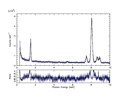
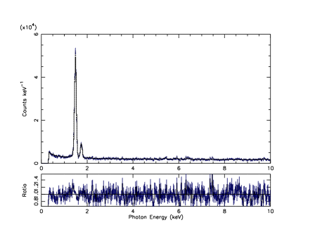
Figure 1.— Typical background model including electronic noise, internal line emission, and particle background from a filter wheel-closed observation in pn (left) and for both MOS detectors (right). The flux is shown in units of counts per 25 eV, with the data shown as dashed lines and the model as solid lines. The ratio of the two is shown in the lower panels. The effective exposure time for the pn exposure is 28 ks, whereas for each MOS exposure it is 23 ks.

3.3.4 Markov Chain Model Sample

In the Monte Carlo, photons are simulated according to the probability functions given by the model parameters, as described in Section 3.1. The simulated photons are propagated through the detector model and binned on the grid determined by the three-dimensional photon density of the data, as described in Section 3.3.1. The two-sample likelihood Poisson statistic is calculated to provide a goodness of fit. In our analysis we use a model-to-data oversimulation factor of 10 for all data sets to reduce the model noise. In principle, it would be ideal to utilize a factor as large as possible, but we are limited by finite CPU speed and internal memory. In PMA07 we compare different values of this factor and show that the results improve significantly when using a value of 10 or greater. Parameters are iterated by Markov chain sampling, as described in the previous Sections.

Figure 2 shows the evolution of the statistic (Poisson $\chi^{2}$/dof.)$-1$. Illustrated are (from left to right) values for the 700 blob run for A1689, the 600 blob run for RX J0658-55 and the 600 blob run for Centaurus. The statistic (Poisson $\chi^{2}$/dof) approaches a value very close to 1 and stabilizes after $\sim 2000$ iterations. The value of the statistic at iteration 2000 for the three data sets (1.005, 1.013 and 1.016) is taken as an indicator that we have achieved an accurate fit.

In the bottom panels of the same figure we show the evolution of the (Poisson $\chi^{2}$/dof)-1 value for the control runs with 100 smoothed particles. In general, the runs with more blobs reach a good fit faster and approach a lower value of the fit statistic. On the basis of these plots we consider the chain to be stable after 2000 iterations, when the statistic becomes stationary and close to 1. We only use samples from iteration 2000 on to deduce cluster properties in the following sections.

Figure 2.— Poisson $\chi^{2}$ per degree of freedom for (top, from left to right), the Abell 1689, RX J0658-5557, and Centaurus standard runs (700,600 and 600 blobs respectively), and (bottom, from left to right) the Abell 1689, RX J0658-5557, and Centaurus 100 blob runs .

4. Final model

To visualize the output model sample we use the methods described in PMA07. We stop the Markov chains after 4000 iterations and assume convergence after 2000 iterations, as described above. We are left with 2000 models, each consistent with the data. Each iteration takes approximately 30 minutes on a single Intel Pentium 4 2.0 GHz CPU which results in about 3 months of computing time per cluster. The models are filtered and marginalized in order to deduce the cluster properties that are discussed below.

4.1. Abell 1689

To confirm that we have an acceptable overall spectral fit, we plot the model spectrum as inferred from the model sample versus the data and the ratio of the two in Figure 3. This plot shows an overall accurate spectral fit with the exception of the instrumental Cu K line, which appears to be detected at a slightly higher energy than expected. This mismatch is most likely due to gain variations in the XMM-Newton CCDs. The accuracy of the fit is seen by looking at the statistic in Figure 2.

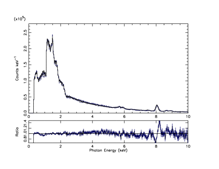
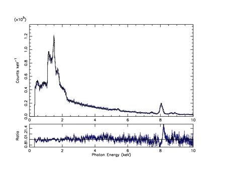
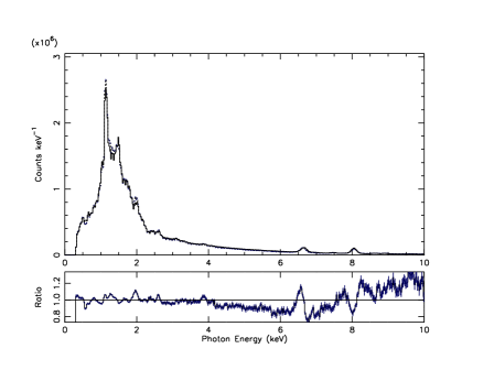
Figure 3.— Spectral comparison of the data (dashed line) to the model (solid line) for the Abell 1689 700 blob analysis (top left), the RX J0658-55 600 blob analysis (top right), and the Centaurus 600 blob analysis (bottom) for the full $20\arcmin\times 20\arcmin$ field used in the analysis. Flux is in units of photon counts per 25 eV bin, with the ratio of data to model shown in the lower panels. The model spectra are produced by averaging the spectrum from every 100th iteration from 2000 to 4000 and are renormalized to match the data counts. The spectra include all backgrounds and all three EPIC detectors.

To infer the luminosity distribution of the cluster, we generate the luminosity map for each model in the sample and take the median in each spatial pixel in order to make the median luminosity map shown in Figure 4 (right). The bolometric luminosity, $L_{bol}$, is displayed in units of $10^{44}~{}$erg s^-1 per $2\arcsec\times 2\arcsec$. The map of raw counts (counts per $2\arcsec\times 2\arcsec$) from the screened data file is shown on the left for comparison. There is good agreement between the reconstruction and the raw data; specifically, the reconstructed profile is sharper than the data due to PSF deconvolution and the fact that obvious chip gaps in the data are compensated by taking the exposure into account.

We have selected three interesting regions (numbered in Figure 4), motivated by our analysis in Andersson & Madejski (2004) to study in more detail the distribution of plasma temperatures in those regions. First, for a cluster that has a quite regular surface brightness distribution, similar to clusters with well-established “cooling cores,” the temperature of the core for Abell 1689 is quite high: $\sim 7.5$ keV. Second, we have identified a region of hotter plasma, $\sim 9$ keV, to the north of the cluster core, indicating possible shock heating of the gas in that region. Third, we have chosen to study in detail a region south of the core exhibiting a temperature almost as low as that of the core itself.

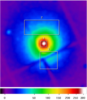
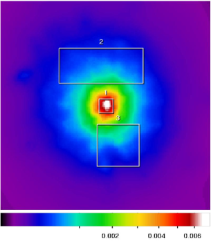
Figure 4.— Results of the analysis for Abell 1689, showing the central $5\arcmin\times 5\arcmin$ region. Left: Raw data smoothed by a $4\arcsec$ kernel Gaussian (counts per $2\arcsec\times 2\arcsec$ pixel). Right: Luminosity reconstruction using the median of all samples at each spatial point ($L_{bol}/10^{44}~{}$erg s^-1 per $2\arcsec\times 2\arcsec$).

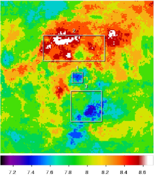
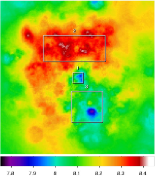
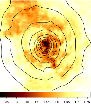
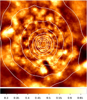
Figure 5.— Results of the analysis for Abell 1689, showing the central $5\arcmin\times 5\arcmin$ region. Top left, temperature map (in units of keV) constructed using the mode of the distribution for all samples at each spatial point; top right, temperature map (in units of keV) constructed using the median of the distribution for all samples at each spatial point; bottom left, temperature uncertainty map (in units of keV) showing the 1 $\sigma$ variation of the temperature mode in the model sample; bottom right, temperature uncertainty map (in units of keV) showing the 1 $\sigma$ variation of the emission-weighted temperature in the model sample.

Next, we form a median temperature map by first weighting the temperature of each model particle by its luminosity, creating a temperature map for each model in the 2000 model MCMC sample. This sample of maps is then averaged by taking the median of the distribution of temperatures for each spatial pixel, as is done in the creation of luminosity maps. Instead of taking the luminosity-weighted average, in another attempt to visualize the distribution of temperatures in the cluster, we bin the luminosity in bins of temperature in each spatial pixel, creating a three dimensional differential luminosity data cube. We do this for all sample models, and for each of them, we calculate the mode of the resulting distribution of each spatial pixel. Taking the median over all model samples of this mode accurately describes the dominant temperature at any given spatial position. We note that this will not give the same value of the temperature as one would get from traditional spectral analysis. The temperature measurement is biased due to the degeneracies present in spectral fitting when allowing for 700 separate temperature phases. However, we believe that it is the method of highest contrast when separating distinct temperature components of a galaxy cluster. The median distribution mode and the median emission-weighted temperature are shown in Figure 5 (top left and top right). To display an estimate of the error on the emission-weighted temperature we calculate the 1 $\sigma$ variation on these quantities over the model sample. These maps are shown in the same figure (bottom left and bottom right). The uncertainty of the emission-weighted temperature is below 0.5 keV throughout most of the shown region. For all of the calculations above we have used the model run with 700 particles.

Figure 6.— Iteration averaged distribution of temperatures for A1689 regions 1 (core; left), 2 (south; middle) and 3 (north, right).

In order to study the regions selected above in more detail, we have extracted the differential luminosity distribution in these regions and binned them into 20 bins over the 5-11 keV allowed range. We have chosen to use the model run with 100 particles for this in order not to over-complicate the problem. While in this case the luminosity and temperature maps do not show the same level of detail, the distributions of spectral parameters become narrower.

The differential luminosity, plotted as the emission measure, $\int{n_{H}n_{e}}$dV, per keV, along with the median of the distribution, is shown for these regions in Figure 6. From these data alone we cannot detect any deviation from isothermality in these regions, mostly due to the inherent degeneracies associated with the attempt to fit high-temperature emission with a multi-phase model. Since most of the emission is from the bremsstrahlung continuum there are many combinations of gas phases (temperatures) that provide equally good fits to the data.

We have confirmed the existence of a region of hot plasma north of the cluster core as we reported in Andersson & Madejski (2004). This hotter plasma appears to extend in an arc approximately halfway around the northern part. The technique verifies both the presence of the colder emission to the south and the lower than ambient (by $\sim 1$ keV) temperature of the cluster core. Our analysis reveals an apparent trail to the south, possibly a remnant tracing the path of the cluster core, and the shock-heated region to the north. However, this could also be due to projection effects from filaments extending in the direction of the line of sight.

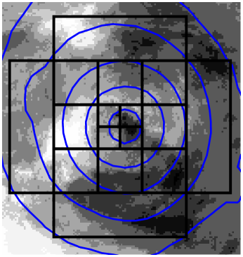
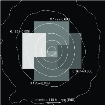
Figure 7.— Left: Redshift map of Abell 1689 obtained by taking the median of the dominant redshift mode over the model sample. The gray scale from black to white corresponds to $z=0.175-0.185$. Superposed contours from the raw event list data and grid regions from Andersson & Madejski (2004) are shown for comparison. Right: Results from the analysis in Andersson & Madejski (2004)

In our earlier findings we infer intra-cluster gas motions from a shift in the position of the Fe K line complex corresponding to $\Delta z\approx 0.01$. Here we show a map of cluster redshift (Figure 7, left) that is similar to the temperature maps shown above. The map was created by calculating the dominant redshift mode at each spatial pixel and taking the median over the samples. The superposed contours are iso-photon count from the raw data, and the grid is shown for comparison with the regions used in Andersson & Madejski (2004). The results from Andersson & Madejski (2004) are shown in Figure 7 (right). The map clearly confirms the $\Delta z\approx 0.01$ east-west gradient found previously by us, corresponding to a velocity of $\sim 3000~{}$km s^-1. We also assess the significance of this by analyzing the redshift-mode variation in the model sample. The $1\sigma$ model variance of the redshift mode in the regions of interest ranges from 0.016 to 0.019, and therefore our result is only $\sim 1\sigma$ significant. Putting an upper threshold on the redshift discrepancy, we find that $\Delta z<0.045$. However, we note that it is not clear that the above is the most appropriate estimate of the true uncertainty, since inherent properties of the method could increase the variance; possibly, another means of error estimation could give a more accurate result. Also, this particular model was not designed specifically to deduce the redshift-structure of the cluster gas. Devising the run only to measure this effect will likely prove more successful.

4.2. RX J0658-55

Similarly to the case of Abell 1689, we plot the model spectrum as inferred from a subsample of the model sample versus the data and the ratio of the two in Figure 3. This plot shows an acceptable fit, again with the exception of the Cu K line complex. The evolution of the Poisson $\chi^{2}$ as a function of Markov chain iteration is shown in Figure 2. As described previously, we generate a median luminosity map from the model and compare it with a counts map smoothed by a $4\arcsec$ Gaussian (Figure 8 right and left). It can be seen that the “bullet” and the main cluster features become somewhat sharper by the PSF deconvolution effect from the forward fitting that is inherent in the method.

We form and plot the luminosity weighted temperature map as well as a map based on the dominant temperature mode, in Figure 9 (top right and top left). In conjunction, the associated uncertainty maps are shown (bottom right and bottom left). Both maps clearly show the cold core remnant of the “bullet” and the hot shocked gas in front of it. Note that the mode and weighted temperature maps display different properties of the temperature structure and are not comparable. This of course is due to the approach used to model the plasma in our method. Instead of using just a single temperature, as is customary, in every spatial region, we use a number of phases that over the model sample form a nearly continuous distribution. We discuss this further in the paragraph discussing isothermal simulations below. The mode is often biased towards lower temperatures for plasmas with temperatures of 9 keV and lower, due to the fact that within the bandpass of EPIC, at higher $T$, the spectra are more similar to each other and therefore are more difficult to distinguish.

We do not see a clear decrease in temperature in front of the shock, as is expected, since the gas should be undisturbed here. It is possible that emission from the post-shock gas is smeared by the XMM-Newton PSF and completely dominates the pre-shock emission, which in turn would be very faint in comparison. The cold gas of the bullet shows an apparent tail stretching south-east from the bullet center. By looking at the temperature map alone, one would conclude that this tail might reveal the movement history of the bullet in the merger. However, the luminosity map and, much more clearly, the 500 ks Chandra exposure (M. Markevitch et al. in preparation), show a symmetrical Mach cone directed westward, indicating that this is the direction of motion. The weak-lensing analysis (Bradac et al., 2006) also shows the western dark matter halo just west of the bullet. It still cannot be ruled out that the bullet core entered to the north-east of the main cluster (see the “entry hole” devoid of emission in this region), proceeding south-west through the main cluster and eventually slingshotting around to the northwest, thus creating the tail visible in the temperature maps. The dark-matter dominated regions and the gas-dominated ones, of course, do not need to have similar merger paths. This scenario is also supported by the apparently previously shock-heated region of gas located directly south of the cluster. This part seems to have almost as hot a gas as the shock in front of the bullet. We select this region (No. 6) along with the six other regions shown in Figure 8, to do a more detailed analysis.

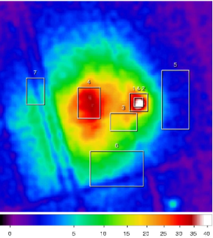
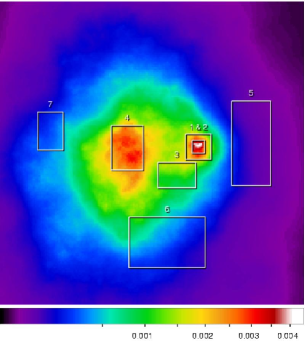
Figure 8.— Results of the analysis for RX J0658-55 showing central $5\arcmin\times 5\arcmin$ region. Left: Raw data smoothed by a $4\arcsec$ kernel Gaussian (counts per $2\arcsec\times 2\arcsec$ pixel). Right: Luminosity reconstruction using the median of all samples at each spatial point ($L_{bol}/10^{44}~{}$erg s^-1 per $2\arcsec\times 2\arcsec$).

In Figure 10 we show the detailed distributions of temperatures, in numerical order, from the selected regions above. In region 1 we have extracted the central emission from the cluster core. The distribution clearly shows the signatures of a $kT=7~{}$keV plasma, with possible contamination from higher temperatures (seen as peaks around 11 and 14 keV), most likely from projection effects. Regions 2-7 show the distributions of various regions in the cluster.

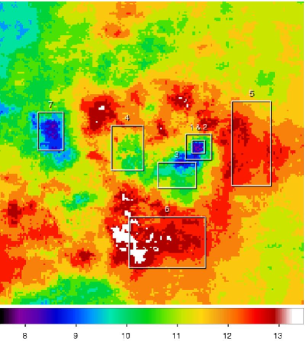
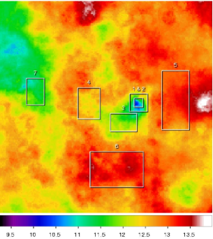
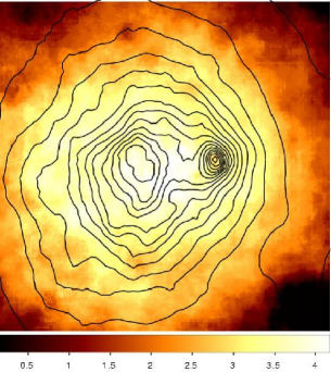
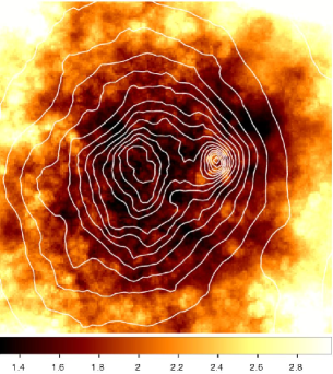
Figure 9.— Results of the analysis for RX J0658-55, showing the central $5\arcmin\times 5\arcmin$ region. Top left, temperature map (in units of keV) constructed using the mode of the distribution for all samples at each spatial point; top right, temperature map (in units of keV) constructed using the median of the distribution for all samples at each spatial point; bottom left, temperature uncertainty map (in units of keV) showing the 1 $\sigma$ variation of the temperature mode in the model sample; bottom right, temperature uncertainty map (in units of keV) showing the 1 $\sigma$ variation of the emission-weighted temperature in the model sample.

In order to determine the deviation from isothermality of the plasma in the selected regions we generated isothermal data sets of a cluster resembling RX J0658-55 with the same number of photons and the same spatial structure. The isothermal models were reconstructed using the exact same method as in the reconstruction of the real data. The distribution of temperatures from the isothermal reconstructions are shown for 4, 7, 10, and 15 keV plasmas in Figure 11. None of the distributions in Figure 10 can conclusively be distinguished from an isothermal plasma.

Figure 10.— Iteration-averaged distribution of temperatures for RX J0658-55 in regions 1-7, also showing the median.

Figure 11.— Iteration-averaged distribution of temperatures for the reconstruction of isothermal simulations of RX J0658-5557 due to 4, 7, 10, and 15 keV plasmas.

Finally we have created luminosity maps of RX J0658-55 using emission components in separate bands of temperature. Figure 12 shows the cluster luminosity in the $kT=1-7$, $7-13$ and $13-19$ keV bands. The contours are iso-luminosity contours from the $kT=1-7$ keV map. These maps show an interesting property hinted at by the temperature maps: the bullet appears to move further north with higher temperature. It is possible that this feature indicates an increased compression to the north-west resulting in a higher temperature. This is supported by the Chandra image which shows a shorter distance between the bullet and shock front to the northwest than to the southwest.

The three-phase map also clearly shows the extension of hotter gas to the south that is causing the high-temperature region in the temperature maps (region 6).

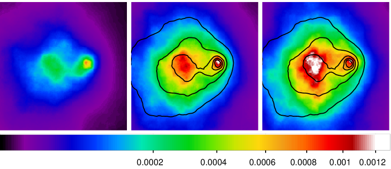
Figure 12.— Luminosity maps ($L_{bol}/10^{44}~{}$erg s^-1 per $2\arcsec\times 2\arcsec$) of RX J0658-55 in three different temperature bands. From left to right, the ranges are 1 - 7, 7 - 13 and 13 - 19 keV.

4.3. The Centaurus Cluster

The model spectrum of the Centaurus cluster as inferred from the model sample is shown with the data spectrum and the ratio of the two in Figure 3. The model spectrum can be seen to fit the data well, and this is a consequence of the fact that we have a low value of the overall Poisson $\chi^{2}$, as can be seen in Figure 2. However, there are some residuals at $>5~{}$keV energies due to some inadequately fitted spectral lines. Since most of the data are in the low-energy range, these data tend to drive the fit, leading to some unwanted excesses and deficits at higher energies. These, however, do not have a major impact on the statistic.

We form both luminosity and temperature maps, analogous to our procedures in previous sections. In Figure 13 the raw count map of the XMM-Newton data (left) is shown as well as the luminosity reconstruction (right). Even though the gaps from dead pixel rows are taken into account via the exposure map, some artifacts can be seen. The model aligns itself with the chip gap where a filament extends north-east of the cluster core. Figure 14 shows a temperature mode map (top left), as well as a median temperature map (top right), with the relevant uncertainty maps shown below. The dominant temperature mode can be seen to be elevated with respect to the median in a hot region north-east in the direction of the filament.

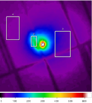
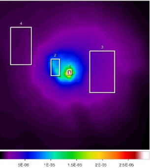
Figure 13.— Results of the analysis for the Centaurus cluster, showing the central $6\arcmin\times 6\arcmin$ region. Left: Raw data smoothed by a $4\arcsec$ kernel Gaussian (counts per $2\arcsec\times 2\arcsec$ pixel). Right: Luminosity reconstruction using the median of all samples at each spatial point ($L_{bol}/10^{44}~{}$erg s^-1 per $2\arcsec\times 2\arcsec$).

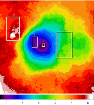
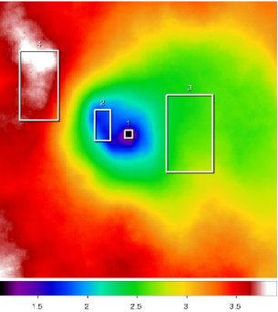
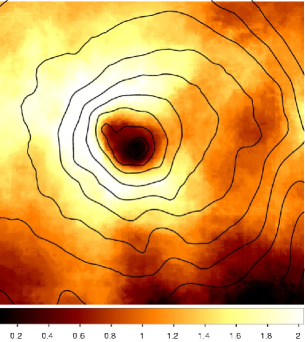
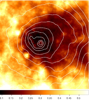
Figure 14.— Results of the analysis for the Centaurus cluster, showing the central $6\arcmin\times 6\arcmin$ region. Top left, temperature map (in units of keV) constructed using the mode of the distribution for all samples at each spatial point; top right, temperature map (in units of keV) constructed using the median of the distribution for all samples at each spatial point; bottom left, temperature uncertainty map (in units of keV) showing the 1 $\sigma$ variation of the temperature mode in the model sample; bottom right, temperature uncertainty map (in units of keV) showing the 1 $\sigma$ variation of the emission weighted temperature in the model sample.

To investigate the temperature in some of the more interesting regions in detail, we calculated the temperature distributions in four regions and compared them. These plots are shown in Figure 15. The order of the regions corresponds to the numbers in Figure 13. Selected regions correspond to the cluster core (No. 1), the extended filament (No. 2), the ambient temperature directly to the west of the core (No. 3), and the anomalously hot region to the north-east (No. 4). The core shows signs of nonisothermality; the distribution includes a narrow peak at 0.5 keV, as well as a bump around 1.5 keV, very probably due to projection. In the other plots it is harder to distinguish the distributions from isothermal. However in region 4 there is a hint of a hotter $\sim 8$keV phase.

Figure 15.— Iteration-averaged distribution of temperatures for Centaurus in regions 1-4 also showing the median.

For the Centaurus cluster we have focused on a new approach in analyzing cluster structure. In Figure 16 we have produced median maps for the luminosity in bands of different temperatures. This is similar to the method of Fabian et al. (2006), who fit a six-phase plasma model to finely spatially binned data of the Perseus cluster in order to make maps of gas mass in six different temperature bands. The main differences with our modeling are that here we use a smooth cluster model and allow for a very large number of variable temperature phases. From left to right, Figure 16 shows the cluster luminosity in the 0 - 1, 1 - 2, 2 - 4, 4 - 6, 6 - 8, and 8 - 10 keV temperature bands.

This subdivision reveals some striking features: the cluster core is dominant in the 0-1 keV band, and apparently it has moved in from the northeast, leaving a tail of colder gas. The 1 - 2 keV temperature band map shows a bi-polar nature of this emission around the core. With higher temperatures, the emission becomes more and more offset, and the 8 - 10 keV map shows a concentration of superheated gas in an isolated region to the north-east, possibly the remnant of a merger. This was noted in the analysis of the Chandra data for this cluster by Crawford et al. (2005). Interestingly, this feature is aligned with a filament extending from the cluster core. Possibly these two irregular phenomena are related.

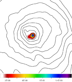
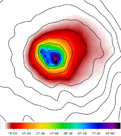
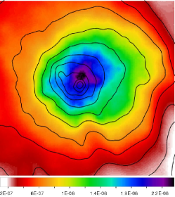
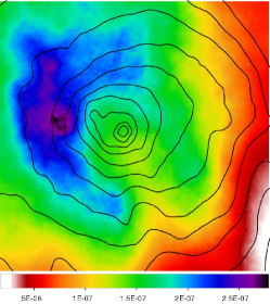
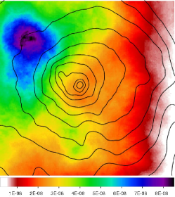
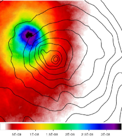
Figure 16.— Luminosity maps ($L_{bol}/10^{44}~{}$erg s^-1 per $2\arcsec\times 2\arcsec$) of the Centaurus cluster in the 0 - 1, 1 - 2, 2 - 4, 4 - 6, 6 - 8 and 8 - 10 keV temperature bands. The superposed contours represent full band luminosity.

Finally, we explore the metallicity structure of Centaurus by creating a median metal abundance map, analogous to our construction of median temperature maps. The metallicity map is shown in Figure 17 and confirms previous findings by Fabian et al. (2005) and Sanders & Fabian (2006) that the metallicity increases by about a factor of 2 (from 0.5 to 1.0 solar) towards the center. However, in contrast to Fabian et al. (2005), we do not find metal abundance levels as high as twice the Solar value and we also do not see a sharp decrease towards 0 in the very center. A minor dip can however, be distinguished. It is most likely that both the absence of very high metallicity and the sharp central feature are due to PSF smearing effects. We also confirm a tight correlation between temperature and metallicity in the gas, with lower temperature plasma generally having a higher metallicity. Calculating the Pearson product-moment correlation coefficient for the median values of temperature and metal abundance per $2\arcsec\times 2\arcsec$ bin, as shown in Figures 14 and 17, weighted by the luminosity in that bin gives a coefficient of $-0.87$, hence confirming a strong correlation. We do not find any significant discrepancy in the spatial distribution of the redshift of the gas, in agreement with Ota et al. (2007).

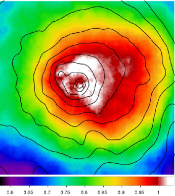
Figure 17.— Metallicity map of the central $6\arcmin\times 6\arcmin$ region of Centaurus showing the metallicity with respect to solar, and with contours representing luminosity.

5. Discussion

This paper describes an application of the Markov chain Monte Carlo technique developed by us for the analysis of observations with the XMM-Newton imaging instruments. We demonstrate the flexibility and power of this technique – employing smoothed particle inference – via studies of three very different clusters, Abell 1689, RX J0658-55 and Centaurus, especially regarding the ability to determine the spatial distribution of temperature of the radiating plasma, which is difficult via more traditional techniques.

We found evidence for cluster merger activity in all these systems, but in each case, the signature was quite distinct. The bullet of RX J0658-55, the remnant of a merger in Centaurus and the asymmetry of temperature in A1689 may roughly correspond to the early, middle, and late stages of cluster merging. In all cases the core of the cluster seemed relatively unaffected. Further systematic studies in temperature structure may add to our understanding of the effect of mergers on cluster properties.

The most important difference of our technique compared to conventional modeling is that we use overlapping emission components. This facilitates the use of a large number of phases describing the X-ray emission at each spatial coordinate. This scenario is much more physical than when one adapts the assumption that any given point in the projected cluster image can be described by a single-temperature phase. However, it also poses the challenge of constraining a distribution of phases when the spectra of high-temperature plasmas in particular are very similar. Comparison with other analyses requires the projection of a distribution into a single value. We have chosen in this paper to show the mode and the median of that distribution in our temperature maps along with the associated 1 $\sigma$ variations (see Figures 5, 9, and 14).

The difference in the assumptions in modeling precludes any direct comparison with other measurements, and it is more than likely that the results will be different. The median of our distributions in particular will depend on the choice of the allowed range of temperatures in the model. This is especially true for the choice of the upper boundary in high-temperature sources. The selection of the boundaries must be based on prior knowledge of the source, such as measurements in the hard X-ray band. This introduces a systematic uncertainty that has to be taken into account.

Another advantage of this technique is the way we treat the background. Since the background is modelled instead of subtracted, difficult aspects of background subtraction, such as weighing the different vignetting of different components, are avoided. The background model has been calibrated against a number of observations in which the filter wheel was closed, as well as against numerous “blank sky” observations (see Section 3.3.3). Even though we allow the normalizations of different background components to be optimized by the MCMC, there is still a small systematic uncertainty associated with residual calibration uncertainties.

In this work we have opted to simultaneously fit the spatial distributions of the temperature, metallicity, and redshift of the X-ray-emitting, plasma illustrating the broad power of the method. This is not necessarily the optimal approach to answer a specific question about the cluster, such as resolving a redshift difference across A1689. This may explain the larger statistical uncertainty obtained in this work compared to our conventional analysis (Andersson & Madejski, 2004). For such a problem the method could be designed specifically for this purpose. Since temperature and metallicity variations are small across this cluster these could be global parameters in the modeling significantly simplifying the overall problem. For such tasks that are highly dependent on detailed spectral features, the number of cluster particles should also be kept to a minimum to avoid the risk of smearing the spectral feature in question. This is, however, a compromise, since a lower number of particles would limit the spatial resolution of the spectral feature that one wants to resolve.

In summary, the statistical uncertainties in this work, which are inherent in problems with large numbers of degrees of freedom, may seem larger than those that are achieved in traditional analyses, but the uncertainties can always be reduced by simplifying the problem. This work attempts to constrain all cluster characteristics into a single model. There will be other applications in which a specific model can be tested to answer a specific problem.

6. Future work

We expect that this method will prove to be powerful in the determination of cluster gas density and entropy. Since the model is multi parametric and analytical, based on the Markov chain posterior, the smoothed particles can be manipulated in order to construct a three-dimensional cluster model. In principle, the $z$-coordinate can be chosen for each particle on the basis of some assumption of spherical symmetry. This can be done separately in ranges of particle plasma temperature, assuming that particles of similar temperatures exhibit the same structure as in the two-dimensional case. This will accurately produce the temperature gradient in the three-dimensional case while preserving the two-dimensional observed structure. This is likely the most accurate method to determine the three-dimensional spectrally resolved structure of galaxy clusters in the X-ray band.

Since the likelihood calculation does not have to be limited to a single instrument, but can potentially include multiple X-ray instruments or even data from other kinds of measurements (such as gravitational lensing, Sunyaev-Zeldovich data, or optical velocity dispersions), the method is quite general. This method is also well suited to analyze other complex, spatially resolved objects where the observed X-ray emission might consist of superposed separable components with varying spectral parameters, such as in supernova remnants.

7. Acknowledgments

We acknowledge many helpful discussions on the suitability of smooth particles for modeling cluster data with Phil Marshall. Financial support for KA is provided by the Göran Gustavsson Foundation for Research in Natural Sciences and Medicine. This work was supported in part by the U.S. Department of Energy under contract number DE-AC02-76SF00515.

References

- Andersson & Madejski (2004) Andersson, K. & Madejski, G. 2004, ApJ 607, 190.
- Arabadjis et al. (2002) Arabadjis, J. S., Bautz, M. W. & Garmire, G. P. 2002, ApJ, 572, 66
- Arnaud et al. (2001) Arnaud, M. et al. 2001, A&A 365, 80.
- Bradac et al. (2006) Bradac, M. et al. 2006, ApJ, 652, 937
- Broadhurst et al. (2005) Broadhurst, T., Takada, M., Umetsu, K., Kong, X., Arimoto, N., Chiba, M., & Futamase, T. 2005, ApJ, 619, L143
- Clowe & Schneider (2001) Clowe, D., & Schneider, P. 2001, A&A, 379, 384
- Clowe et al. (2004) Clowe, D., Gonzalez, A., & Markevitch, M. 2004, ApJ, 604, 596
- Clowe et al. (2006) Clowe, D., Bradac, M., Gonzalez, A., Markevitch, M., Randall, S., Jones, C., & Zaritsky, D. 2006 ApJ, 648, 109
- Crawford et al. (2005) Crawford, C. S., Hatch, N. A., Fabian, A. C., & Sanders, J. S. 2005, MNRAS, 363, 216
- Dickey & Lockman (1990) Dickey, J. M., & Lockman, F. J. 1990, ARA&A 28, 215.
- Ehle et al. (2006) Ehle, M., et al. 2006, XMM-Newton Users’ Handbook, Issue 2.4 (Madrid: ESA), http://xmm.vilspa.esa.es/external/xmm_user_support/documentation/
- Fabian et al. (1981) Fabian, A. C., Hu, E. M., Cowie, L. L., & Grindlay, J. 1981, ApJ, 248, 47
- Fabian et al. (2005) Fabian, A. C., Sanders, J. S., Taylor, G. B., & Allen, S. W. 2005, MNRAS, 360, L20
- Fabian et al. (2006) Fabian, A. C., Sanders, J. S., Taylor, G. B., Allen, S. W., Crawford, C. S., Johnstone, R. M., & Iwasawa, K. 2006, MNRAS, 366, 417
- Finoguenov et al. (2005) Finoguenov, A., Böhringer, H., & Zhang, Y.-Y. 2005, A & A 442, 827.
- Fukazawa et al. (1994) Fukazawa, Y., Ohashi, T., Fabian, A. C., Canizares, C. R., Ikebe, Y., Makishima, K., Mushotzky, R. F., & Yamashita, K. 1994, PASJ, 46, L55
- Fukazawa et al. (1998) Fukazawa, Y., Makishima, K., Tamura, T., Ezawa, H., Xu, H., Ikebe, Y., Kikuchi, K., & Ohashi, T. 1998, PASJ, 50, 187
- Hickox & Markevitch (2006) Hickox, R. C., & Markevitch, M. 2006, ApJ, 645, 95
- Jansen et al. (2001) Jansen, F., et al. 2001, A&A, 365, L1
- Kaastra et al. (2004) Kaastra, J. S. et al. 2004, A & A 413, 414.
- Kaastra (1992) Kaastra, J. S. 1992, An X-Ray Spectral Code for Optically Thin Plasmas (Internal SRON-Leiden Report, ver. 2.0)
- King et al. (2002) King, L. J., Clowe, D. I., & Schneider, P. 2002, A&A, 383, 118
- Kirsch (2006) Kirsch, M. 2006, EPIC Status of Calibration and Data Analysis (XMM-SOC-CAL-TN-0018; Madrid: ESA), http://xmm.vilspa.esa.es/external/xmm_sw_cal/calib/
- Liang et al. (2000) Liang, H., Hunstead, R. W., Birkinshaw, M., & Andreani, P. 2000, ApJ, 544, 686
- Liang et al. (2001) Liang, H., Ekers, R. D., Hunstead R.W., Falco E.E., & Shaver P. 2001, MNRAS, 328, L21
- Liedahl et al. (1995) Liedahl, D. A., Osterheld, A. L., & Goldstein, W. H. 1995, ApJ, 438, L115
- Lokas et al. (2006) Lokas, E., Prada, F., Wojtak, R., Moles, M., & Gottlober, S. 2006, MNRAS, 366, L26
- Lumb (2002) Lumb, D. H., EPIC Background Files (XMM-SOC-CAL-TN-0016; Madrid: ESA)
- Markevitch et al. (2000) Markevitch, M. et al., 2000, ApJ 541, 542
- Markevitch et al. (2002) Markevitch, M., Gonzalez, A.H., David, L., Vikhlinin, A., Murray, S., Forman, W., Jones, C., & Tucker, W. 2002, ApJ 567, L27
- Mewe et al. (1985) Mewe, R., Gronenschild, E. H. B. M., & van den Oord, G. H. J. 1985, A&AS, 62, 197
- Mewe et al. (1986) Mewe, R., Lemen, J. R., & van den Oord, G. H. J. 1986, A&AS, 65, 511
- Miralda-Escude & Babul (1995) Miralda-Escude, J., & Babul, A. 1995, ApJ, 449, 18
- Morrison & McCammon (1983) Morrison, R. & McCammon, D. 1983, ApJ, 270, 119
- Ota et al. (2007) Ota, N., et al. 2007, PASJ, 59, 351
- Petrosian et al. (2006) Petrosian, V., Madejski, G., & Luli, K. 2006, ApJ, 652, 948
- Peterson et al. (2001) Peterson, J. R. et al. 2001, A & A 365, L104.
- Peterson et al. (2004) Peterson, J. R., Jernigan, J. G., & Kahn, S. M. 2004, ApJ 615, 545
- Peterson, Marshall, & Andersson (2007) Peterson, J. R., Marshall P. J., & Andersson, K. E. 2007, ApJ 655, 109 (PMA07)
- Pratt & Arnaud (2002) Pratt, G. W. & Arnaud, M. 2002, A & A 394, 375
- Read et al. (2005) Read, A. M., Sembay, S. F., Abbey, T. F., & Turner, M. J. L. 2005, in The X-ray Universe 2005, ed. A Wilson (ESA-SP 604; Noordwijk: ESA), 925
- Sanders et al. (2004) Sanders, J. S., Fabian, A. C., Allen, S. W., & Schmidt, R. W. 2004, MNRAS 349, 952.
- Sanders & Fabian (2006) Sanders, J. S., & Fabian, A. C. 2006, MNRAS, 371, 1483
- Tucker et al. (1995) Tucker, W. H., Tananbaum, H., & Remillard, R. A. 1995, ApJ, 444, 532
- Tucker et al. (1998) Tucker, W. et al. 1998, ApJ, 496, L5
- Turner et al. (2001) Turner, M. J. L., et al. 2001, A&A, 365, L27
- Tyson & Fischer (1995) Tyson, J. A., & Fischer, P. 1995, ApJ, 446, L55
- Zhang et al. (2004) Zhang, Y.-Y., Finoguenov, A., Böhringer, H., Ikebe, Y., Matsushita, K., & Schuecker, P. 2004, A & A 413, 49.